5

Simulation-Based Markov Decision Processes

Markov decision processes (MDPs) model decision-making in situations where outcomes are partly random and partly under the control of a decision maker. MDP is a stochastic process characterized by five elements: decision epochs, states, actions, transition probability, and reward. The characteristic elements of a Markovian process are the states in which the system finds itself and the available actions that the decision maker can carry out in that state. These elements identify two sets: the set of states in which the system can be found and the set of actions available for each specific state. The action chosen by the decision maker determines a random response from the system, which brings it into a new state. This transition returns a reward that the decision maker can use to evaluate the merit of their choice. In this chapter, we will learn how to deal with decision-making processes with Markov chains. We will analyze the concepts underlying Markovian processes and then analyze some practical applications to learn how to choose the right actions for the transition between different states of the system.

In this chapter, we’re going to cover the following main topics:

• Introducing agent-based models
• Overview of Markov processes
• Introducing Markov chains
• Markov chain applications
• The Bellman equation explained
• Multi-agent simulation
• Schelling’s model of segregation

Technical requirements

In this chapter, MDPs will be introduced. In order to deal with the topics in this chapter, it is necessary that you have a basic knowledge of algebra and mathematical modeling.

To work with the Python code in this chapter, you’ll need the following files (available on GitHub at the following URL: https://github.com/PacktPublishing/Hands-On-Simulation-Modeling-with-Python-Second-Edition):

• simulating_random_walk.py
• weather_forecasting.py
• schelling_model.py

Introducing agent-based models

Agent-based simulation (ABM) is a class of computational models aimed at the computer simulation of actions and interactions of autonomous agents to evaluate their effects on the overall system. ABMs incorporate intelligent elements capable of learning, adapting, evolving, or following unpredictable logic. One of the key features, which turns out to be one of the strengths of this methodology, is the bottom-up approach, which, considering the interactions of the individual elements of the system, tries to determine the emergent characteristics produced by these interactions. These characteristics are not explicit of the system but emerge from the interaction of the group of agents who act independently, are oriented towards achieving their specific goal, and interact in a shared environment.

The applications of ABM are many and particularly useful. They are usually used to study phenomena that are too complex to be faithfully reproduced and/or expensive in terms of cost and effort. For example, the study of the behavior of a population bounded in a certain area, as well as the simulation of reactions between molecules in a chemical solution, or even the management of distributed systems that can be represented as nodes of a network that request and offer services. The reason for the increasing use of ABMs is to be found in the growing complexity of the networks with which a system can be modeled. The organizational, temporal, and economic costs for the analytical study of such systems would be too high; moreover, the experiment itself could prove to be risky. This tool allows us to study and analyze the dynamic behavior of a real system through the behavior of an artificial system.

An ABM is characterized by three fundamental components:

• Agents: Autonomous entities with their own characteristics and behaviors
• Environment: A field in which agents interact with each other
• Rules: They define the actions and reactions that occur during the simulation

An ABM assumes that only local information is available to agents. The ABM is a decentralized system; there is no central entity that globally disseminates the same information to all agents or controls their behavior with the aim of increasing the performance of the system. Agents interact with each other, but they don’t all interact at the same time together. The interaction between them typically occurs with a sub-group of similar entities close to each other (neighbors). Similarly, the interaction between them and the environment is also localized; in fact, it is not certain that the agents interact with every part of the environment.

Therefore, the information obtained by the agents is obtained from the sub-group with which they interact and from the portion of the environment in which they are located. If the model is not static, the sub-group and the environment with which an agent interacts vary over time. The agent of an ABM interacts with others of its kind and with the environment. This plays a fundamental role in the simulation and is represented in such a way as to reproduce the context in which the real event occurs. It usually keeps the positional information of the agents over time to be able to keep track of all the movements made during the execution of the simulation.

There may also be objects in the field: they represent specific areas of the environment that have different characteristics depending on their location. Agents can interact with them to manipulate, produce, destroy, or be influenced by them and change behavior.

Some essential characteristics of ABMs are summarized in the following points:

• They define the decision-making processes of individual agents, considering both social and economic aspects
• They incorporate the influence of decisions made at the micro level by linking them to the consequences at the macro level
• They study the overall response generated by a change in the environment or the policies implemented

The ABM-based approach must be built and validated with the participation of the various stakeholders present within the model. In this way, the ABM promotes the collective learning process by integrating local and scientific knowledge, providing further information and assistance to policymakers in defining the most suitable policies for solving a specific problem.

Through ABM, it is possible to identify structures and patterns that emerge at the macroscopic level because of the interactions between agents at the microscopic level. No agent possesses the emergent properties of the system; these properties cannot be obtained as the sum of the individual behaviors of the single agents.

The complexity of a system is due to the interaction between the agents that develops at the microscopic level, which determines their characteristics at the macroscopic level. These interactions develop over time by linking the states of the system to each other in a chain of events. In Markov processes, the information obtainable from the observation of the history of the process up to the present can be useful for making inferences about the future state.

In the next section, we will study these processes to fully understand how agent-based models are structured.

Overview of Markov processes

Markov’s decision-making process is defined as a discrete-time stochastic control process. In Chapter 2, Understanding Randomness and Random Numbers, we said that stochastic processes are numerical models used to simulate the evolution of a system according to random laws. Natural phenomena are characterized by random factors both in their very nature and observation errors. These factors introduce a random number into the observation of the system. This random factor determines an uncertainty in the observation since it is not possible to predict with certainty what the result will be. In this case, we can only say that it will assume one of the many possible values with a certain probability.

If starting from an instant t in which an observation of the system is made, the evolution of the process will depend only on t, while it will not be influenced by the previous instants. Here, we can say that the stochastic process is Markovian.

Important note

A process is called Markovian when the future evolution of the process depends only on the instant of observation of the system and does not depend in any way on the past.

Characteristic elements of a Markovian process include the states in which the system finds itself and the available actions that the decision maker can carry out in that state. These elements identify two sets: the set of states in which the system can be found and the set of actions available for each specific state. The action chosen by the decision maker determines a random response from the system, which brings it into a new state. This transition returns a reward that the decision maker can use to evaluate the goodness of their choice.

The agent-environment interface

A Markovian process takes on the characteristics of an interaction problem between two elements to achieve a goal. The two characteristic elements of this interaction are the agent and the environment. The agent is the element that must reach the goal, while the environment is the element that the agent must interact with. The environment corresponds to everything that is external to the agent.

The agent is a piece of software that performs the services necessary for another piece of software in a completely automatic and intelligent way. They are known as intelligent agents.

The essential characteristics of an agent are listed here:

• The agent continuously monitors the environment, and this action causes a change in the state of the environment
• The available actions belong to a continuous or discrete set
• The agent’s choice of action depends on the state of the environment
• This choice requires a certain degree of intelligence as it is not trivial
• The agent has a memory of the choices made – intelligent memory

The agent’s behavior is characterized by attempting to achieve a specific goal. To do this, it performs actions in an environment it does not know a priori, or at least not completely. This uncertainty is filled through the interaction between the agent and the environment. In this phase, the agent learns to know the state of the environment by measuring it, in this way, planning its future actions.

The strategy adopted by the agent is based on the principles of error theory: proof of the actions and memory of the possible mistakes made to make repeated attempts until the goal is achieved. These actions by the agent are repeated continuously, causing changes in the environment that change their state.

Important note

Crucial to the agent’s future choices is the concept of reward, which represents the environment’s response to the action taken. This response is proportional to the weight that the action determines in achieving the objective: it will be positive if it leads to correct behavior, while it will be negative in the case of an incorrect action.

The decision-making process that leads the agent to achieve their objective can be summarized in three essential points:

• The objective of the agent
• Their interaction with the environment
• The total or partial uncertainty of the environment

In this process, the agent receives stimuli from the environment through the measurements made by sensors. The agent decides what actions to take based on the stimuli received from the environment. As a result of the agent’s actions, determining a change in the state of the environment will receive a reward.

The crucial elements in the decision-making process are shown in the following diagram:

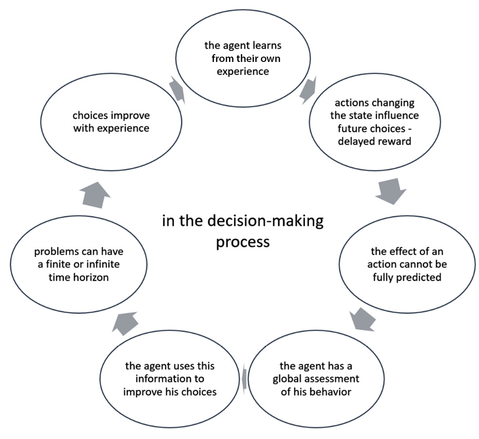
Figure 5.1 – The agent’s decision-making process

While choosing an action, it is crucial to have a formal description of the environment. This description must return essential information regarding the properties of the environment and not a precise representation of the environment.

Exploring MDPs

The agent-environment interaction we discussed in the previous section is approached as a Markov decision-making process. This choice is dictated by loading problems and computational difficulties. As anticipated in the Overview of Markov processes section, Markov’s decision-making process is defined as a discrete-time stochastic control process.

Here, we need to perform a sequence of actions, with each action leading to a non-deterministic change regarding the state of the environment. By observing the environment, we know its state after performing an action. On the other hand, if the observation of the environment is not available, we do not know the state, even after performing the action. In this case, the state is a probability distribution of all the possible states of the environment. In such cases, the change process can be viewed as a snapshot sequence.

The state at time t is represented by a random variable st. Decision-making is interpreted as a discrete-time stochastic process. A discrete-time stochastic process is a sequence of random variables xt, with t ∈ N. We can define some elements as follows:

• State space: Set of values that random variables can assume
• History of a stochastic process (path): The realization of the sequence of random variables

The response of the environment to a certain action is represented by the reward. The agent-environment interaction in an MDP can be summarized by the following diagram:

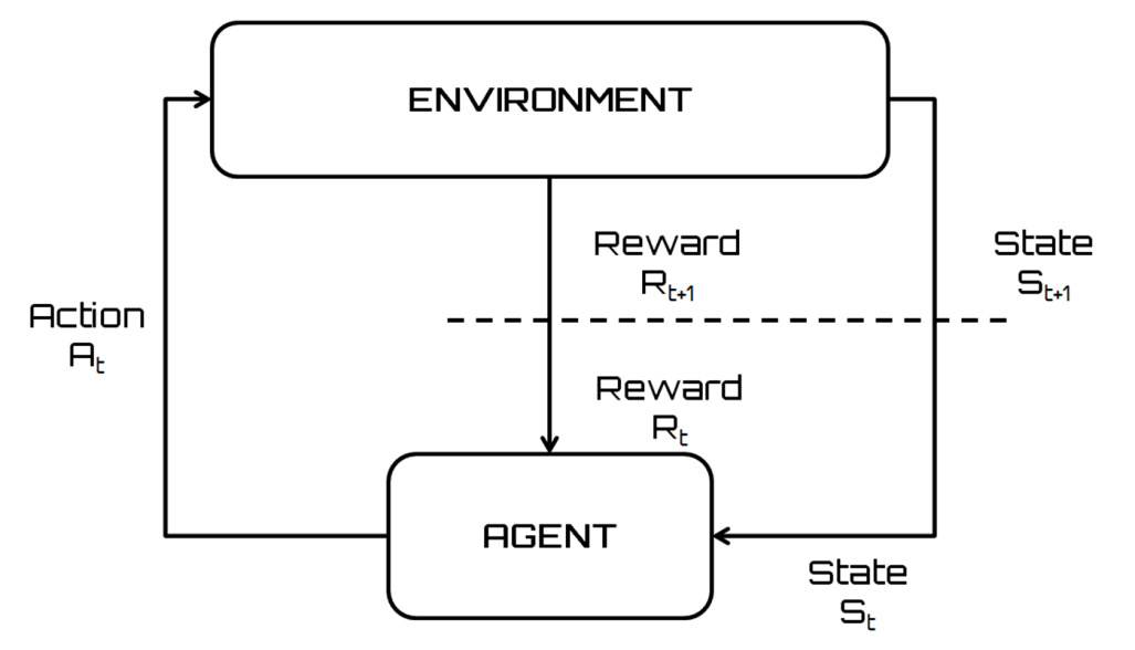
Figure 5.2 – The agent-environment interaction in MDP

The essential steps of the agent-environment interaction, schematically represented in the previous diagram, are listed here:

1. The interaction between the agent and the environment occurs at discrete instants over time.
2. In every instant, the agent monitors the environment by obtaining its state st ∈ S, where S is the set of possible states.
3. The agent performs an action a ∈ A (st), where A (st) is the set of possible actions available for the state st.
4. The agent chooses one of the possible actions according to the objective to be achieved.
5. This choice is dictated by the policy π (s, a), which represents the probability that the action a is performed in the state s.
6. At time t + 1, the agent receives a numerical reward rt + 1 ∈ R corresponding to the action previously chosen.
7. Because of the choice, the environment passes into the new state.
8. The agent must monitor the state of the environment and perform a new action.
9. This iteration repeats until the goal is achieved.

In the iterative procedure we have described, the state st + 1 depends on the previous state and the action taken. This feature defines the process as an MDP, which can be represented by the following equation:

In the previous equation, δ represents the state function. We can summarize an MDP as follows:

• The agent monitors the state of the environment and has a series of actions
• At a discrete time t, the agent detects the current state and decides to perform an action at ∈ A
• The environment reacts to this action by returning a reward rt = r (st, at) and moving to the state st + 1 = δ (st, at)

Important note

The r and δ functions are characteristics of the environment that depend only on the current state and action. The goal of MDP is to learn a policy that, for each state of the system, provides the agent with an action that maximizes the total reward accumulated during the entire sequence of actions.

Now, let’s analyze some of the terms that we introduced previously. They represent crucial concepts that help us understand Markovian processes.

The reward function

A reward function identifies the target in a Markovian process. It maps the states of the environment detected by the agent by enclosing it in a single number, which represents the reward. The purpose of this process is to maximize the total reward that the agent receives over the long term because of their choices. Then, the reward function collects the positive and negative results obtained from the actions chosen by the agent and uses them to modify the policy. If an action selected based on the indications provided by the policy returns a low reward, then the policy will be modified to select other actions. The reward function performs two functions: it stimulates the efficiency of the decisions and determines the degree of risk aversion of the agent.

Policy

A policy determines the agent’s behavior in terms of decision-making. It maps both the states of the environment and the actions to be chosen in those states, representing a set of rules or associations that respond to a stimulus. The policy is the fundamental part of a Markovian agent as it determines its behavior. In a Markov decision-making model, a policy provides a solution that associates a recommended action with each state potentially achievable by the agent. If the policy provides the highest expected utility among the possible actions, it is called an optimal policy (π*). In this way, the agent does not have to keep their previous choices in memory. To make a decision, the agent only needs to execute the policy associated with the current state.

The state-value function

The value function provides us with the information necessary to evaluate the quality of a state for an agent. It returns the value of the expected goal that was obtained following the policy of each state, which is represented by the total expected reward. The agent depends on the policy to choose the actions to be performed.

Understanding the discounted cumulative reward

The goal of MDP is to learn a policy that guides an agent in choosing the actions to be performed for each state of the environment. This policy aims to maximize the total reward received during the entire sequence of actions performed by the agent. Let’s learn how to maximize this total reward. The total reward that’s obtained from adopting a policy is calculated as follows:

In the preceding equation, rT is the reward of the action that brings the environment into the terminal state sT.

To get the maximum total reward, we can select the action that provides the highest reward for each individual state, which leads to the choice of the optimal policy that maximizes the total reward.

Important note

This solution is not applicable in all cases, for example, when the goal or terminal state is not achieved in a finite number of steps. In this case, both Rt and the sum of the rewards you want to maximize tend to infinity.

An alternative technique uses the discounted cumulative reward, which tries to maximize the following amount:

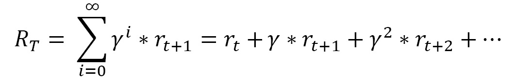
In the previous equation, γ is called the discount factor and represents the importance of future rewards. The discount factor is 0 ≤ γ ≤ 1 and has the following conditions:

• γ <1: The sequence rt converges to a finite value
• γ = 0: The agent does not consider future rewards, thereby trying to maximize the reward only for the current state
• γ = 1: The agent will favor future rewards over immediate rewards

The value of the discount factor may vary during the learning process to take special actions or states into account. An optimal policy may include individual actions that return low rewards, provided that the total reward is higher.

Comparing exploration and exploitation concepts

Upon reaching the goal, the agent looks for the most rewarded behavior. To do this, they must link each action to the reward returned. In the case of complex environments with many states, this approach is not feasible due to many action-reward pairs.

Important note

This is the well-known exploration-exploitation dilemma: for each state, the agent explores all possible actions, exploiting the action most rewarded in achieving the objective.

Decision-making requires a choice between the two available approaches:

• Exploitation: The best decision is made based on current information
• Exploration: The best decision is made by gathering more information

The best long-term strategy can impose short-term sacrifices as this approach requires collecting adequate information to reach the best decisions.

In everyday life, we often find ourselves having to choose between two alternatives that, at least theoretically, lead to the same result: this approach is an exploration-exploitation dilemma. For example, let’s say we need to decide whether to choose what we already know (exploitation) or choose something new (exploration). Exploitation keeps our knowledge unchanged, while exploration makes us learn more about the system. It is obvious that exploration exposes us to the risk of wrong choices.

Let’s look at an example of using this approach in a real-life scenario: we must choose the best path to reach our trusted restaurant:

• Exploitation: Choose the path you already know
• Exploration: Try a new path

In complex problems, converging toward an optimal strategy can be too slow. In these cases, a solution to this problem is represented by a balance between exploration and exploitation.

An agent who acts exclusively based on exploration will always behave randomly in each state with convergence to an optimal strategy that is practically impossible. On the contrary, if an agent acts exclusively based on exploitation, they will always use the same actions, which may not be optimal.

Let’s now introduce the Markov chains that describe a stochastic process whose evolution depends exclusively on the immediately preceding state.

Introducing Markov chains

Markov chains are discrete dynamic systems that exhibit characteristics attributable to Markovian processes. These are finite state systems – finite Markov chains – in which the transition from one state to another occurs on a probabilistic, rather than deterministic, basis. The information available about a chain at the generic instant t is provided by the probabilities that it is in any of the states, and the temporal evolution of the chain is specified by specifying how these probabilities update by going from the instant t at instant t + 1.

Important note

A Markov chain is a stochastic model in which the system evolves over time in such a way that the past affects the future only through the present: Markov chains have no memory of the past.

A random process characterized by a sequence of random variables X = X0, ..., Xn with values in a set j0, j1, ..., jn is given. This process is Markovian if the evolution of the process depends only on the current state, that is, the state after n steps. Using conditional probability, we can represent this process with the following equation:

If a discrete-time stochastic process X has a Markov property, it is called the Markov chain. A Markov chain is said to be homogeneous if the following transition probabilities do not depend on n and only on i and j:

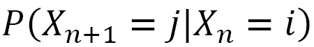
In such hypotheses, let’s assume we have the following:

All joint probabilities can be calculated by knowing the numbers pij and the following initial distribution:

This probability represents the distribution of the process at zero time. The probabilities pij are called transition probabilities, and pij is the probability of transitioning from I to j in each time phase.

Transition matrix

The application of homogeneous Markov chains is made easy by adopting the matrix representation. Through this, the formula expressed by the previous equation becomes much more readable. We can represent the structure of a Markov chain through the following transition matrix:

This is a positive matrix in which the sum of the elements of each row is unitary. In fact, the elements of the ith row are the probabilities that the chain, being in the state Si at the instant t, passes through S1 or S2,. . . or Sn at the next instant. Such transitions are mutually exclusive and exhaustive of all possibilities. Such a positive matrix with unit sum lines is stochastic. We will call each vector positive line x stochastic such that T = [x1 x2. . . xn], in which the sum of the elements assumes a unit value:

The transition matrix has the position (i, j) to pass from result i to result j by performing a single experiment.

Transition diagram

The transition matrix is not the only solution for describing a Markov chain. An alternative is an oriented graph called a transition diagram, in which the vertices are labeled by the states S1, S2, ..., Sn, and there is a direct edge connecting the vertex Si to the vertex Sj, if and only if, the probability of transition from Si to Sj is positive.

Important note

The transition matrix and the transition diagram contain the same information necessary for representing the same Markov chain.

Le’’s take a look at an example: consider a Markov chain with three possible states, 1, 2, and 3, represented by the following transition matrix:

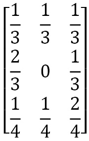
As mentioned previously, the transition matrix contains the same information as the transition diagram. Let’s learn how to draw this diagram. There are three possible states, 1, 2, and 3, and the direct boundary from each state to other states shows the probabilities of transition pij. When there is no arrow from state i to state j, this means that pij = 0:

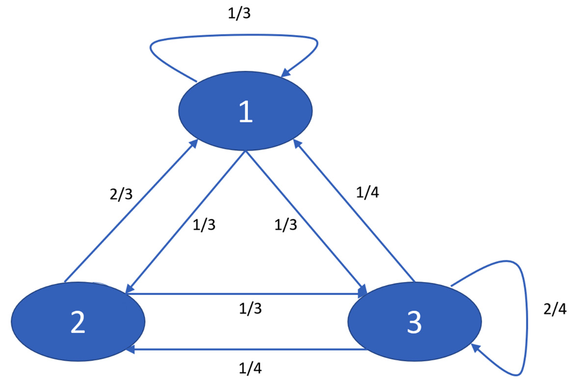
Figure 5.3 – Diagram of the transition matrix

In the preceding transition diagram, the arrows that come out of a state always add up to exactly 1, just like for each row in the transition matrix.

After having introduced the Markov chains, we now see some practical cases of the application of this methodology.

Markov chain applications

Now, let’s look at a series of practical applications that can be made using Markov chains. We will introduce the problem and then analyze the Python code that will allow us to simulate how it works.

Introducing random walks

Random walks identify a class of mathematical models used to simulate a path consisting of a series of random steps. The complexity of the model depends on the system features we want to simulate, which are represented by the number of degrees of freedom and the direction. The authorship of the term is attributed to Karl Pearson, who, in 1905, first referred to the term casual walk. In this model, each step has a random direction that evolves through a random process involving known quantities that follow a precise statistical distribution. The path that’s traced over time will not necessarily be descriptive of real motion: it will simply return the evolution of a variable over time. This is the reason for the widespread use of this model in all areas of science: chemistry, physics, biology, economics, computer science, and sociology.

One-dimensional random walk

The one-dimensional casual walk simulates the movement of a punctual particle that is bound to move along a straight line, thus having only two movements: right and left. Each movement is associated with a random shift of one step to the right with a fixed probability p or to the left with a probability q. Every single step is the same length and is independent of the others. The following diagram shows the path to which the punctual particle is bound, along with the direction and the two verses allowed:

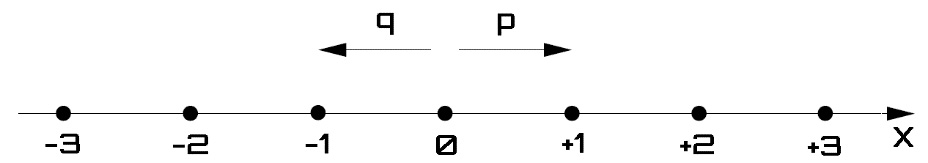
Figure 5.4 – One-dimensional walk

After n passes, the position of the point will be identified by its abscissa X (n), characterized by a random term. Our aim is to calculate the probability with which the particle will return to the starting point, after n steps.

Important note

The idea that the point will actually return to its starting position is not assured. To represent the position of the point on the straight line, we will adopt the X (n) variable, which represents the abscissa of the line after the particle has moved n steps. This variable is a discrete random variable with a binomial distribution.

The path of the point particle can be summarized as follows: for each instant, the particle moves one step to the right or left according to the value returned by a random variable Z (n). This random variable takes only two dichotomous values:

• +1 with probability p> 0
• -1 with probability q

The two probabilities are related to each other through the following equation:

Let’s consider random variables Zn with n = 1, 2, …. Suppose that these variables are independent and with equal distribution. The position of the particle at instant n will be represented by the following equation:

In the previous formula, Xn is the next value in the walk, Xn-1 is the observation in the previous time phase, and Zn is the random fluctuation in that step.

Important note

The Xn variable identifies a Markov chain; that is, the probability that the particle in the next moment is in a certain position depends only on the current position, even if we know all the moments preceding the current one.

Simulating a 1D random walk

The simulation of a casual walk does not represent a trivial succession of random numbers since the next step to the current one represents its evolution. The dependence between the next two steps guarantees a certain consistency from one passage to the next. This is not guaranteed in a banal generation of independent random numbers, which instead return big differences from one number to another. Let’s learn how to represent the sequence of actions to be performed in a simple casual walking model through the following pseudocode:

1. Start from the 0 position.
2. Randomly select a dichotomous value (-1, 1).
3. Add this value to the previous time step.
4. Repeat step 2 onward.

This simple iterative process can be implemented in Python by processing a list of 1,000 time steps for the random walk. Let’s take a look:

1. Let’s start by loading the necessary libraries:

   from random import seed

   from random import random

   from matplotlib import pyplot

The random module implements pseudo-random number generators for various distributions. The random module is based on the Mersenne Twister algorithm. Mersenne Twister is a pseudorandom number generator. Originally developed to produce inputs for Monte Carlo simulations, almost uniform numbers are generated via Mersenne Twister, making it suitable for a wide range of applications.

From the random module, two libraries were imported: seed and random. In this code, we will generate random numbers. To do this, we will use the random() function, which produces different values each time it is invoked. It has a very large period before any number is repeated. This is useful for producing unique values or variations, but there are times when it is useful to have the same dataset available for processing in different ways. This is necessary to ensure the reproducibility of the experiment. To do this, we can use the random.seed() function contained in the seed library. This function initializes the basic random number generator.

The matplotlib library is a Python library for printing high-quality graphics. With matplotlib, it is possible to generate graphs, histograms, bar graphs, power spectra, error graphs, scatter graphs, and so on with a few commands. This is a collection of command-line functions like those provided by the MATLAB software.

2. Now, we will investigate the individual operations. Let’s start with setting the seed:

   seed(1)

The random.seed() function is useful if we wish to have the same set of data available to be processed in different ways, as this makes the simulation reproducible.

Important note

This function initializes the basic random number generator. If you use the same seed in two successive simulations, you will always get the same sequence of pairs of numbers.

3. Let’s move on and initialize the crucial variable of the code:

   RWPath= list()

The RWPath variable represents a list that will contain the sequence of values representative of the random walk. A list is an ordered collection of values, which can be of various types. It is an editable container, meaning that we can add, delete, and modify existing values. For our purposes, where we want to continuously update our values through the subsequent steps of the path, the list represents the most suitable solution. The list() function accepts a sequence of values and converts them into lists. With the preceding command, we simply initialized the list that is currently empty, and with the following code, we start to populate it:

RWPath.append(-1 if random() < 0.5 else 1)

The first value that we add to our list is a dichotomous value. It is simply a matter of deciding whether the value to be added is 1 or -1. The choice, however, is made on a random basis. Here, we generate a random number between 0 and 1 using the random() function and then check if it is <0.5. If it is, then we add -1, otherwise, we add 1. At this point, we will use an iterative cycle with a for loop, which will repeat the procedure for 1,000 steps:

for i in range(1, 1000):

At each step, we will generate a random term as follows:

     ZNValue = -1 if random() < 0.5 else 1

Important note

As we did when we chose the first value to add to the list, we generate a random value with the random() function, so if the value that’s returned is lower than 0.5, the ZNValue variable assumes the value -1; otherwise, 1.

4. Now, we can calculate the value of the random walk at the current step:

   XNValue = RWPath[i-1] + ZNValue

The XNValue variable represents the value of the abscissa in the current step. It is made up of two terms: the first represents the value of the abscissa in the previous state, while the second is the result of generating the random value. This value must be added to the list:

RWPath.append(XNValue) 

This procedure will be repeated for the 1,000 steps that we want to perform. At the end of the cycle, we will have the entire sequence stored in the list.

5. Finally, we can visualize it through the following piece of code:

   pyplot.plot(RWPath)

   pyplot.show()

The pyplot.plot() function plots the values contained in the RWPath list on the y axis using x as an index array with the following value: 0..N-1. The plot() function is extremely versatile and will take an arbitrary number of arguments.

Finally, the pyplot.show() function displays the graph that’s created, as follows:

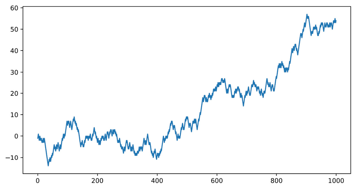
Figure 5.5 – The trend plot of the random walk path

In the previous graph, we can analyze the path followed by the point particle in a random process. This curve can describe the trends of a generic function, not necessarily associated with a road route. As anticipated, this process is configured as a Markovian process in that the next step is independent of the position from the previous step and depends only on the current step. The casual walk is a mathematical model widely used in finance. In fact, it is widely used to simulate the efficiency of information deriving from the markets: the price varies for the arrival of new information, which is independent of what we already know.

Simulating a weather forecast

Another potential application of Markov chains is in the development of a weather forecasting model. Let’s learn how to implement this algorithm in Python. To start, we can work with a simplified model: we will consider only two climatic conditions/states, that is, sunny and rainy. Our model will assume that tomorrow’s weather conditions will be affected by today’s weather conditions, making the process take on Markovian characteristics. This link between the two states will be represented by the following transition matrix:

The transition matrix returns the conditional probabilities P (A | B), which indicate the probability that event A occurs after event B has occurred. This matrix, therefore, contains the following conditional probabilities:

In the previous transition matrix, each row contains a complete distribution. Therefore, all the numbers must be non-negative, and the sum must be equal to 1. The climatic conditions show a tendency to resist change. For this reason, after a sunny day, the probability of another sunny-P (Sunny | Sunny) day is greater than a rainy-P (Sunny | Rainy) day. The climatic conditions of tomorrow are not directly related to those of yesterday; it follows that the process is Markovian. The previous transition matrix is equivalent to the following:

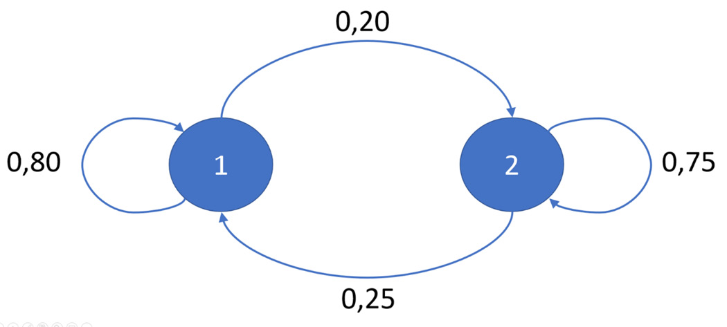
Figure 5.6 – Transition diagram

The simulation model we want to elaborate on will have to calculate the probability that it will rain in the next few days. It will also have to allow you to recover a statistic of the proportion between sunny and rainy days in a certain period of time. The process, as mentioned previously, is Markovian, and the tools we analyzed in the previous sections allow us to obtain the requested information. Let’s get started:

1. Let’s see the Python code that alternates sunny and rainy days, starting from a specific initial condition. As always, we will analyze it line by line, starting with loading the necessary libraries:

   import numpy as np

   import matplotlib.pyplot as plt

The numpy library is a Python library that contains numerous functions that can help us manage multidimensional matrices. Furthermore, it contains a large collection of high-level mathematical functions we can use on these matrices. We will use two functions: random.seed() and random.choose().

The matplotlib library is a Python library for printing high-quality graphics. With matplotlib, it is possible to generate graphs, histograms, bar graphs, power spectra, error graphs, scatter graphs, and so on with a few commands. It is a collection of command-line functions like those provided by the MATLAB software. Let’s move on and illustrate the code:

np.random.seed(3)

The random.seed() function initializes the seed of the random number generator. In this way, the simulation that uses random numbers will be reproducible. The reproducibility of the experiment will be guaranteed by the fact that the random numbers that will be generated will always be the same.

2. Now, let’s define the possible states of the weather conditions:

   StatesData = ["Sunny","Rainy"]

Two states are provided: sunny and rainy. The transitions matrix representing the transition between the weather conditions will be set as follows:

TransitionStates = [["SuSu","SuRa"],["RaRa","RaSu"]]
TransitionMatrix = [[0.80,0.20],[0.25,0.75]]

The transition matrix returns the conditional probabilities P (A | B), which indicate the probability that event A occurs after event B has occurred. All the numbers in a row must be non-negative and the sum must be equal to 1. Let’s move on and set the variable that will contain the list of state transitions:

WeatherForecasting = list()

The WeatherForecasting variable will contain the results of the weather forecast. This variable will be of the list type.

Important note

A list is an ordered collection of values and can be of various types. It is an editable container and allows us to add, delete, and modify existing values.

For our purpose, which is to continuously update our values through the subsequent steps of the path, the list represents the most suitable solution. The list() function accepts a sequence of values and converts them into lists.

3. Now, we decide on the number of days for which we will predict the weather conditions:

   NumDays = 365

For now, we have decided to simulate the weather forecast for a 1-year time horizon; that is, 365 days. Let’s fix a variable that will contain the forecast for the current day:

TodayPrediction = StatesData[0]

Furthermore, we also initialized it with the first vector value containing the possible states. This value corresponds to the Sunny condition. We print this value on the screen by doing the following:

print("Weather initial condition =",TodayPrediction)

At this point, we can predict the weather conditions for each of the days set by the NumDays variable. To do this, we will use a for loop that will execute the same piece of code several times equal to the number of days that we have set in advance:

for i in range(1, NumDays):

Now, we will analyze the main part of the entire program. Within the for loop, the forecast of the time for each consecutive day occurs through an additional conditional structure: the if statement. Starting from a meteorological condition contained in the TodayPrediction variable, we must predict that of the next day. We have two conditions: sunny and rainy. In fact, there are two control conditions, as shown in the following code:

if TodayPrediction == "Sunny":        
        TransCondition = np.random.choice(TransitionStates[0],replace=True,p=TransitionMatrix[0])
        if TransCondition == "SuSu":
            pass
        else:
            TodayPrediction = "Rainy"
           
 elif TodayPrediction == "Rainy":
        TransCondition = np.random.choice (TransitionStates[1],replace=True,p=TransitionMatrix[1])
        if TransCondition == "RaRa":
            pass
        else:
            TodayPrediction = "Sunny"

• If the current state is Sunny, we use the numpy random.choice() function to forecast the weather condition for the next state. A common use for random number generators is to select a random element from a sequence of enumerated values, even if these values are not numbers. The random.choice() function returns a random element of the non-empty sequence passed as an argument. Three arguments are passed:
• TransitionStates[0]: The first row of the transition states
• replace=True: The sample is with replacement
• p=TransitionMatrix[0]: The probabilities associated with each entry in the state passed

The random.choice() function returns random samples of the SuSu, SuRa, RaRa, and RaSu types, according to the values contained in the TransitionStates matrix. The first two will be returned starting from sunny conditions and the remaining two starting from rainy conditions. These values will be stored in the TransCondition variable.

Within each if statement, there is an additional if statement. This is used to determine whether to update the current value of the weather forecast or to leave it unchanged. Let’s see how:

if TransCondition == "SuSu":
            pass
        else:
            TodayPrediction = "Rainy" 

If the TransCondition variable contains the SuSu value, the weather conditions of the current day remain unchanged. Otherwise, it is replaced by the Rainy value. The elif clause performs a similar procedure, starting from the rainy condition. At the end of each iteration of the for loop, the list of weather forecasts is updated, and the current forecast is printed:

WeatherForecasting.append(TodayPrediction) 
print(TodayPrediction)

Now, we need to predict the weather forecast for the next 365 days.

4. Let’s draw a graph with the sequence of forecasts for the next 365 days:

   plt.plot(WeatherForecasting)

   plt.show()

The following graph is printed:

Figure 5.7 – Plot of the weather forecast

Here, we can see that the forecast of sunny days prevails over the rainy ones.

Important note

The flat points at the top represent all the sunny days, while the dips in-between are the rainy days.

To quantify this prevalence, we can draw a histogram. In this way, we will be able to count the occurrences of each condition:

plt.figure()
plt.hist(WeatherForecasting)
plt.show()

The following is a histogram of the weather condition for the next 365 days:

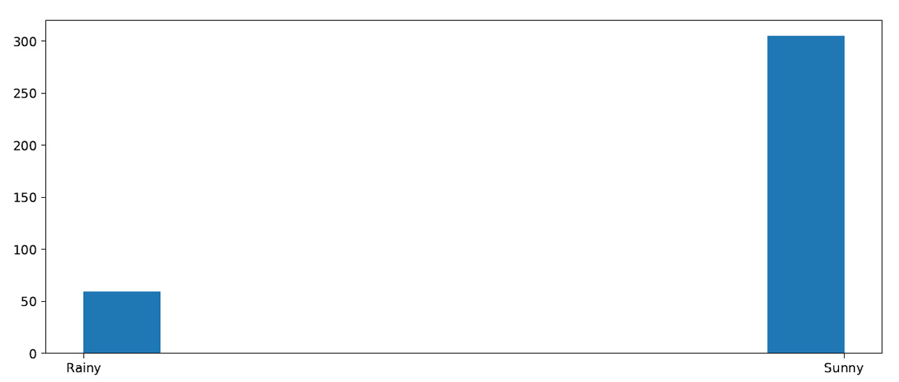
Figure 5.8 – Histogram of the weather forecast

With this, we can confirm the prevalence of sunny days. The result we’ve obtained derives from the transition matrix. In fact, we can see that the probability of the persistence of a solar condition is greater than that of rain. In addition, the initial condition has been set to the sunny condition. We can also try to see what happens when the initial condition is set to the rainy condition.

Bellman equation explained

In 1953, Richard Bellman introduced the principles of dynamic programming in order to efficiently solve sequential decision problems. In such problems, decisions are periodically implemented and influence the size of the model. In turn, these influence future decisions. The principle of optimality, enunciated by Bellman, allows you, through an intelligent application, to efficiently deal with the complexity of the interaction between the decisions and the sizes of the model. Dynamic programming techniques were also applied from the outset to problems in which there is no temporal or sequential aspect.

Important note

Although dynamic programming can be applied to a wide range of problems by providing a common abstract model, from a practical point of view, many problems require models of such dimensions to preclude, then as now, any computational approach. This inconvenience was then called the curse of dimensionality and was an anticipation, still in informal terms, of concepts of computational complexity.

The greatest successes of dynamic programming have been obtained in the context of sequential decision models, especially of the stochastic type, such as the Markovian decision processes, but also in some combinatorial models.

Dynamic programming concepts

Dynamic programming (DP) is a programming technique designed to calculate an optimal policy based on a perfect model of the environment in the form of a Markov decision-making process (MDP). The basis of dynamic programming is the use of state values and action values in order to identify good policies.

DP methods are applied to MDP using two processes called policy evaluation and policy improvement, which interact with each other:

• Policy evaluation: Is done through an iterative process that seeks to solve Bellman’s equation. The convergence of the process for k → ∞ imposes approximation rules, thus introducing a stop condition.
• Policy improvement: Improves the policy based on current values.

In the policy iteration technique, the two phases just described alternate, and each concludes before the other begins.

Important note

The iterative process, when evaluating policies, obliges us to evaluate a policy at each step through an iterative process whose convergence is not known a priori and depends on the starting policy. To address this problem, we can stop evaluating the policy at some point while still ensuring that we converge to an optimal value.

Principle of optimality

The validity of the dynamic optimization procedure is ensured by Bellman’s principle of optimality: An optimal policy has the property that whatever the initial state and initial decision are, the remaining decisions must constitute an optimal policy with regard to the state resulting from the first decision.

Based on this principle, it is possible to divide the problem into stages and solve the stages in sequence, using the dynamically determined values of the objective function, regardless of the decisions that led to them. This allows us to optimize one stage at a time, reducing the initial problem to a sequence of smaller subproblems, therefore, easier to solve.

Bellman equation

Bellman’s equation helps us solve MDP by finding the optimal policy and value functions. The optimal value function V * (S) is the one that returns the maximum value of a state. This maximum value is the one that corresponds to the action that maximizes the reward value of the optimal action in each state. It then adds a discount factor multiplied by the value of the next state by the Bellman equation through a recursive procedure. The following is an example of a Bellman equation:

In the previous equation, we have the following:

• is the function value at state s
• is the reward we get after acting a in state s
• γ is the discount factor
• is the function value at the next state

For a stochastic system, when we take an action, it is not said that we will end up in a later state, but that we can only indicate the probability of ending up in that state.

In everyday life, we know that unity makes strength; we can think that even an intelligent system can benefit from the joint action of several intelligent agents. Making multiple agents operate in a single environment is not an easy thing, so let’s see how to model this interaction and see what benefits we can derive from it.

Multi-agent simulation

An agent can be defined as anything that is able to perceive an environment through sensors and act in it through actuators. Artificial intelligence focuses on the concept of a rational agent, or an agent who always tries to optimize an appropriate performance measure. A rational agent can be a human agent, a robotic agent, or a software agent. In the following diagram, we can see the interaction between the agent and the environment:

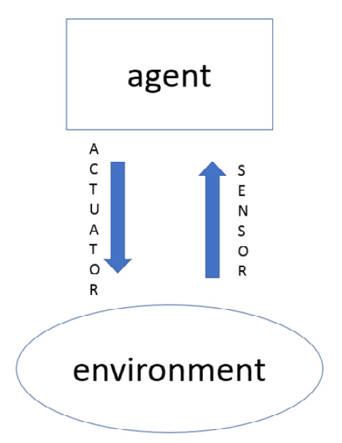
Figure 5.9 – Interaction between the agent and the environment

An agent is considered autonomous when it can flexibly and independently choose the actions to be taken to achieve its goals without constantly resorting to the intervention of an external decision system. Note that, in most complex domains, an agent can only partially obtain information and have control in the environment that it has been inserted into, thus exerting, at most, a certain influence on it.

An agent can be considered autonomous and intelligent if it has the following characteristics:

• Reactivity: It must perceive the environment, managing to adapt in good time to the changes that take place
• Proactivity: It must show behavior oriented toward achieving the objectives set with initiative
• Social skills: It must be able to interact with other agents for the pursuit of its goals

There are numerous situations where multiple agents coexist in the same environment and interact with each other in different ways. In fact, it is quite rare for an agent to represent an isolated system. We can define a multi-agent system (MAS) as a group of agents that can potentially interact with each other. An MAS can be competitive, which is where each agent tries to exclusively maximize their own interests, even at the expense of those of others, rather than cooperative, which is where agents are willing to give up part of their objectives in an attempt to maximize the global utility of the system.

The types of possible interactions are as follows:

• Negotiation: This occurs when agents must seek an agreement on the value to be assigned to some variables
• Cooperation: This occurs when there are common goals for which agents try to align and coordinate their actions
• Coordination: This is a type of interaction aimed at avoiding situations of conflict between agents

The use of MAS systems introduces a series of advantages:

• Efficiency and speed: Thanks to the possibility of performing computations in parallel
• Robustness: The system can overcome single-agent failures
• Flexibility: Adding new agents to the system is extremely easy
• Modularity: Extremely useful in the software design phase due to the possibility of reusing the code
• Cost: The single-unit agent has a very low cost compared to the overall system

The growing attention that’s being paid to multi-agent systems for the treatment of problems based on decision-making processes is linked to some characteristics that distinguish them, such as flexibility and the possibility of representing independent entities through distinct computational units that interact with each other. The various stakeholders of a decision-making system can, in fact, be modeled as autonomous agents. Several practical applications of the real world have recently adopted an approach based on problems such as satisfying and optimizing distributed constraints and identifying regulations that have an intermediate efficiency between the centralized (optimal) and the non-coordinated (bad) ones.

Schelling’s model of segregation

Schelling’s model, which earned Schelling the Nobel Prize in 1979, models the social segregation of two populations of individuals who can move within a city by obeying a few simple rules:

• Each agent is satisfied with their position if there is at least a consistent percentage of neighbors like them around them
• Otherwise, the agents move

The neighbors are, for example, those of the Moore neighborhood, which is its eight closest neighbors. By letting the system evolve according to these rules, it is shown that starting from a mixed population, we obtain a city segregated into neighborhoods in which there are individuals of a single population. This phenomenon has been interpreted as an emergent property as it is typical of the macro scale of the system. It is not due to any centralized control or to explicit decisions by the two groups as a whole, and there is no direct causal link between the rules on individual agents (micro) and the aggregate result of the evolution of the system (macro).

Schelling’s model of segregation, thanks to a model with cellular automata, studies how territorial segregation evolves given two types of agents who prefer to live in areas where they are not a minority. In the segregation model, the formation of segregated neighborhoods is analyzed, giving a territorial notion to the concept of a social group. Schelling considers a population of agents randomly distributed on a plane: the characterization of the agents is general, and the analysis can concern any dichotomous distinction of the population. The agents want to occupy an area where at least 50% of the neighbors are the same color as them. Neighbors are agents who occupy the squares adjacent to the agent’s area under consideration.

Each zone can be occupied by only one agent. The agent’s utility function can be formalized as follows:

q∈0.1 is the share of agents like the agent among its neighbors. Agents can move from area to area. This happens if both of the following conditions apply:

• The current area is mainly inhabited by agents of the same type > 0.5
• There is an adjacent free area

A third condition can be added:

• There is an adjacent free zone that is more satisfactory

This condition could represent the hypothesis that the move is expensive and is carried out only if it brings an improvement. The third condition, by limiting movements, reduces segregation without, however, eliminating it.

Schelling’s result is that the population segregates into areas of homogeneous color, although the preference does not require segregation, such as agents are happy to live in areas where the population is divided exactly in half between the two types or in general in areas in which they are not a minority. Each agent that moves influences the utility of the agents it leaves and the agents it encounters, creating a chain reaction.

Python Schelling model

Now let’s see a practical example of how to implement Schelling’s model in Python. Suppose we have two types of agents: A and B. The two types of agents can represent any two groups in any context. To begin, we place the two populations of agents in random positions in a delimited area. After placing all the agents in the grid, each cell is either occupied by an agent of the two groups or is empty.

Our task will then be to check whether each agent is satisfied with their current position. An agent is satisfied if they are surrounded by at least a percentage of agents of the same type: this threshold will apply to all agents in the model. The higher the threshold, the greater the likelihood that agents are dissatisfied with their current position.

If an agent is not satisfied, they can be moved to any free position on the grid. The choice of the new position can be made by adopting several strategies. For example, a random position can be chosen, or the agent can move to the nearest available position.

You can find the Python code on GitHub as schelling_model.py.

As always, we analyze the code line by line:

1. Let’s start by importing the libraries:

   import matplotlib.pyplot as plt

   from random import random

The matplotlib library is a Python library for printing high-quality graphics. Then, we imported the random() function from the random module. The random module implements PRNGs for various distributions (see the Random number generation using Python section from Chapter 2, Understanding Randomness and Random Numbers).

2. Let’s now define the class that contains the methods for managing agents:

   class SchAgent:

       def __init__(self, type):

           self.type = type

           self.ag_location()

The first method (__init__) allows us to initialize the attributes of the class and will be called automatically when an object of the SchAgent class is instantiated:

    def ag_location(self):
        self.location = random(), random()

The second method (ag_location) defines the location of the agents. In this case, we have chosen to place the agents in a random position; in fact, we have used the random() function. The random() function returns the next nearest floating-point value from the generated sequence. All return values are enclosed between 0 and 1.0. This means that we are going to place our agents on a 1.0 X 1.0 grid:

    def euclidean_distance(self, new):
        eu_dist = ((self.location[0] - new.location[0])**2 
        + (self.location[1] - new.location[1])**2)**(1/2)
        return eu_dist

The third method (euclidean_distance) simply calculates the distance between the agents. To do this, we used the Euclidean distance defined as follows:

    def satisfaction(self, agents):
        eu_dist = []    
        for agent in agents:
            if self != agent:
                eu_distance =     
                     self.euclidean_distance(agent)
                eu_dist.append((eu_distance, agent))
        eu_dist.sort()
        neigh_agent = [agent for k, agent in 
                                        eu_dist[:neigh_num]]
        neigh_itself = sum(self.type == agent.type 
                           for agent in neigh_agent)
        return neigh_itself >= neigh_threshold

The fourth method (satisfaction) evaluates the degree of satisfaction of the agent. As we anticipated, an agent is satisfied if they are surrounded by at least a percentage of agents of the same type: this threshold will apply to all agents in the model. This threshold will then be set when we are going to define the simulation parameters of the model:

    def update(self, agents):
        while not self.satisfaction(agents):
            self.ag_location()

The last method (update) moves the agent’s position in case they are not satisfied.

3. After defining the methods for the SchAgent class, we now need to define the function that will allow us to view the evolution of the model. In this way, we will be able to verify how the agents move on the grid:

   def grid_plot(agents, step):

       x_A, y_A = [], []

       x_B, y_B = [], []

       for agent in agents:

           x, y = agent.location

           if agent.type == 0:

               x_A.append(x)

               y_A.append(y)

           else:

               x_B.append(x)

               y_B.append(y)

       fig, ax = plt.subplots(figsize=(10, 10))

       ax.plot(x_A, y_A, '^', markerfacecolor='b',markersize= 10)

       ax.plot(x_B, y_B, 'o', markerfacecolor='r',markersize= 10)

       ax.set_title(f'Step number = {step}')

       plt.show()

The function creates vectors x and y for each type of agent and inserts the current position. Next, create a chart with the location of each agent. To better appreciate the position of the two types of agents, we have denoted the two types of agents with blue triangles for type A and with red circles for type B.

4. Now we can define the simulation parameters:

   num_agents_A = 500

   num_agents_B = 500

   neigh_num = 8      

   neigh_threshold = 4 

We have defined the number of agents of the two types (num_agents_A, num_agents_B). The other two parameters require a more detailed description. The neigh_num variable defines the next neighbors; to set them, we used Moore’s neighborhood definition, such as its eight closest neighbors. The neigh_threshold variable defines the satisfaction threshold; in this case, we requested that satisfaction is obtained when the agent is surrounded by at least 50% of agents of the same type.

5. Now we can instantiate objects:

   agents = [SchAgent(0) for i in range(num_agents_A)]

   agents.extend(SchAgent(1) for i in range(num_agents_B))
6. We then move on to run the simulation:

   step = 0

   k=0

   while (k<(num_agents_A + num_agents_B)):

       print('Step number = ', step)

       grid_plot(agents, step)

       step += 1

       k=0

       for agent in agents:

           old_location = agent.location

           agent.update(agents)

           if agent.location == old_location:

               k=k+1 

   else:

       print(f'Satisfied agents with 

                        {neigh_threshold/neigh_num*100}

                         % of similar neighbors') 

To do this, we used a while loop that checks a k counter. The variable k simply counts the number of satisfied agents; therefore, if the number of satisfied agents is less than the total number of agents, a new update of the agent positions is performed. The cycle, on the other hand, stops when the positions of all the agents remain unchanged.

The following output is printed on the screen:

Step number =  0
Step number =  1
Step number =  2
Step number =  3
Step number =  4
Satisfied agents with 50.0 % of similar neighbors

The evolution of the model is appreciable in the diagrams that are returned. To show the evolution, we compared the initial grid in which the random positions of all agents are shown with the final grid in which all people are satisfied (Figure 5.10).

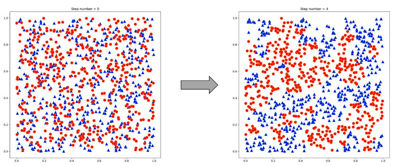
Figure 5.10 – Comparison between the initial and final agent’s position

We can see that in the grid on the left, the agents belonging to the two groups are positioned randomly. On the contrary, in the grid on the right, the agents are grouped into groups of the same type.

Summary

In this chapter, we learned the basic concepts of the Markov process. This is where the future evolution of the process depends only on the instant of observation of the system and in no way depends on the past. We have seen how an agent and the surrounding environment interact and the elements that characterize its actions. We now understand the reward and policy concepts behind decision-making. We then went on to explore Markov chains by analyzing the matrices and transition diagrams that govern their evolution.

Then, we addressed some applications to put the concepts we’d learned about into practice. We dealt with a casual walk and a forecast model of weather conditions by adopting an approach based on Markov chains. Next, we studied Bellman equations as coherence conditions for optimal value functions to determine optimal policy. We also introduced multi-agent systems, which allow us to consider different stakeholders in a decision-making process.

Finally, we studied Schelling’s segregative models with an example of Python code in which two types of agents randomly positioned in a grid are repositioned, creating groups of the same type.

In the next chapter, we will understand how to obtain robust estimates of confidence intervals and standard errors of population parameters, as well as how to estimate the distortion and standard error of a statistic. We will then discover how to perform a test for statistical significance and how to validate a forecast model.