
6
Resampling Methods
Resampling methods are a set of techniques used to repeat data sampling – they simply rearrange the data to estimate the accuracy of a statistic. If we are developing a simulation model and we get unsatisfactory results, we can try to reorganize the starting data to remove any wrong correlations and re-check the capabilities of the model. Resampling methods are one of the most interesting inferential applications of stochastic simulations and random numbers. They are particularly useful in the nonparametric field, where the traditional inference methods cannot be correctly applied. They generate random numbers to be assigned to random variables or random samples. They require machine time related to the growth of repeated operations. They are very simple to implement and once implemented, they are automatic. The required elements must be placed in a sample that is, or at least can be, representative of the population. To achieve this, all the characteristics of the population must be included in the sample. In this chapter, we will try to extrapolate the results obtained from the representative sample of the entire population. Given the possibility of making mistakes in this extrapolation, it will be necessary to evaluate the degree of accuracy of the sample and the risk of arriving at incorrect predictions. In this chapter, we will learn how to apply resampling methods to approximate some characteristics of the distribution of a sample to validate a statistical model. We will analyze the basics of the most common resampling methods and learn how to use them by solving some practical cases.
In this chapter, we’re going to cover the following main topics:
- Introducing resampling methods
- Exploring the Jackknife technique
- Demystifying bootstrapping
- Applying bootstrapping regression
- Explaining permutation tests
- Performing a permutation test
- Approaching cross-validation techniques
Technical requirements
In this chapter, we will address resampling method technologies. To deal with the topics in this chapter, you must have a basic knowledge of algebra and mathematical modeling. To work with the Python code in this chapter, you’ll need the following files (available on GitHub at the following URL: https://github.com/PacktPublishing/Hands-On-Simulation-Modeling-with-Python-Second-Edition):
- jakknife_estimator.py
- bootstrap_estimator.py
- bootstrap_regression.py
- permutation_test.py
- kfold_cross_validation.py
Introducing resampling methods
Resampling methods are a set of techniques based on the use of subsets of data, which can be extracted either randomly or according to a systematic procedure. The purpose of this technology is to approximate some characteristics of the sample distribution – a statistic, a test, or an estimator – to validate a statistical model.
Resampling methods are one of the most interesting inferential applications of stochastic simulations and the generation of random numbers. These methods became widespread during the 1960s, originating from the basic concepts of Monte Carlo methods. The development of Monte Carlo methods took place mainly in the 1980s, following the progress of information technology and the increase in the power of computers. Their usefulness is linked to the development of non-parametric methods, in situations where the methods of classical inference cannot be correctly applied.
The following details can be observed from resampling methods:
- They repeat simple operations many times
- They generate random numbers to be assigned to random variables or random samples
- They require more machine time as the number of repeated operations grows
- They are very simple to implement and once implemented, they are automatic
Over time, various resampling methods have been developed and can be classified based on some characteristics.
Important note
A first classification can be made between methods based on randomly extracting subsets of sample data and methods in which resampling occurs according to a non-randomized procedure.
Further classification can be performed as follows:
- The bootstrap method and its variants, such as subsampling, belong to the random extraction category
- Procedures such as Jackknife and cross-validation fall into the non-randomized category
- Statistical tests, called permutation or exact tests, are also included in the family of resampling methods
Sampling concepts overview
Sampling is one of the fundamental topics of all statistical research. Sampling generates a group of elementary units, that is, a subset of a population, with the same properties as the entire population, at least with a defined risk of error.
By population, we mean the set, finite or unlimited, of all the elementary units to which a certain characteristic is attributed, which identifies them as homogeneous.
Important note
For example, this could be the population of temperature values in each place, in a period that can be daily, monthly, or yearly.
Sampling theory is an integral and preparatory part of statistical inference, along with the resulting sampling techniques, and allows us to identify the units whose variables are to be analyzed.
Statistical sampling is a method used to randomly select items so that every item in a population has a known, non-zero probability of being included in the sample. Random selection is considered a powerful means of building a representative sample that, in its structure and diversity, reflects the population under consideration. Statistical sampling allows us to obtain an objective sample: the selection of an element does not depend on the criteria defined for reasons of research convenience or availability and does not systematically exclude or favor any group of elements within a population.
In random sampling, associated with the calculation of probabilities, the following actions are performed:
- The results are extrapolated through mathematical formulas and an estimate of the associated error is provided
- Control is given over the risk of reaching an opposite conclusion to reality
- The minimum sample size necessary is calculated – through a formula – to obtain a given level of accuracy and precision
Reasoning about sampling
Now, let’s learn why it may be preferable to analyze the data of a sample rather than that of the entire population:
- Consider a case in which the statistical units do not present variability. A statistical unit represents a single element of a set of elements studied, so it represents the smallest element to which a methodology is applied. Here, it is useless to make many measurements because the population parameters are determined with few measurements. A statistical population is a set of items that have been collected to perform a specific experiment. For example, if we wanted to determine the average of 1,000 identical statistical units, this value will be equal to that obtained if we only considered 10 units.
Important note
Sampling is used if not all the elements of the population are available. For example, investigations into the past can only be done on available historical data, which is often incomplete.
- Sampling is indicated when a considerable amount of time is saved when achieving results. This is because even if electronic computers are used, the data-entry phase is significantly reduced if the investigation is limited to a few elements of the overall population.
Pros and cons of sampling
When information is collected, a survey is performed on all the units that make up the population under study. When an analysis is carried out on the information collected, it is only possible to use it on part of the units that make up the population.
The pros of sampling are as follows:
- Cost reduction
- Reduction of time
- Reduction of the organizational load
The disadvantages of sampling are as follows:
- The sampling base is not always available or easy to know
Sampling can be performed by forced choice in cases where the reference population is partially unknown in terms of composition or size. Sampling cannot always replace a complete investigation, such as in the case of surveys regarding the movement of marital status, births, and deaths: all individual cases must be known.
Probability sampling
In probability sampling, the probability that each unit of the population must be extracted is known. In contrast, in non-probability sampling, the probability that each unit of the population must be extracted is not known.
Let’s take a look at an example. If we extract a sample of university students by drawing lots from those present on any day in university, we do not get a probabilistic sample for the following reasons: non-attending students have no chance of entering, and the students who attend the most are more likely to be extracted than the other students of the following years.
How sampling works
The sampling procedure involves a series of steps that need to be followed appropriately to extract data that can adequately represent the population. Sampling is carried out as follows:
- Define the objective population in the detection statistics.
- Define the sampling units.
- Establish the size of the sample.
- Choose the sample or samples on which the la will be statistical detection according to a method of sampling.
- Finally, formulate a judgment on the goodness of the sample.
Now that we’ve adequately introduced the various sampling techniques, let’s look at a practical case.
Exploring the Jackknife technique
This method is used to estimate characteristics such as the distortion and the standard deviation of a statistic. This technique allows us to obtain the desired estimates without necessarily resorting to parametric assumptions. A statistical parameter is a value that defines an essential characteristic of a population, so it is essential for its description. Jackknife is based on calculating the statistics of interest for the sub-samples we’ve obtained, leaving out one sample observation at a time. The Jackknife estimate is consistent for various sample statistics, such as mean, variance, correlation coefficient, maximum likelihood estimator, and others.
Defining the Jackknife method
The Jackknife method was proposed in 1949 by M. H. Quenouille who, due to the low computational power of the time, created an algorithm that requires a fixed number of operations.
Important note
The main idea behind this method is to cut a different observation from the original sample each time and to re-evaluate the parameter of interest. The estimate will be compared with the same one that was calculated on the original sample.
Since the distribution of the variable is not known, the distribution of the estimator is not known either.
Jackknife samples are constructed by leaving an observation, xi, out of the original sample each time, as shown in the following equation:

Then, n samples of size m = n-1 are obtained. Let’s take a look at an example. Consider a sample of size n = 5 that produces five Jackknife samples of size m = 4, as follows:

The pseudo-value, ![]() , is recalculated on the generic i-th sample Jackknife. The procedure is iterated n times on each of the available Jackknife samples:
, is recalculated on the generic i-th sample Jackknife. The procedure is iterated n times on each of the available Jackknife samples:

The following diagram shows this preliminary procedure:

Figure 6.1 – Representation of the Jackknife method
To calculate the variance of the Jackknife estimate, the following equation must be used:

In the previous equation, the term  is defined as follows:

The calculated standard deviation will be used to build confidence intervals for the parameters.
To evaluate and possibly reduce the estimator distortion, the Jackknife estimate of the distortion is calculated as follows:

Essentially, the Jackknife method reduces bias and evaluates variance for an estimator.
Estimating the coefficient of variation
To make comparisons regarding variability between different distributions, we can use the coefficient of variation (CV) since it considers the average of the distribution. The variation coefficient is a relative measure of dispersion and is a dimensionless magnitude. It allows us to evaluate the dispersion of the values around the average, regardless of the unit of measurement.
Important note
For example, the standard deviation of a sample of income expressed in dollars is completely different from the standard deviation of the same income expressed in euros, while the dispersion coefficient is the same in both cases.
The coefficient of variation is calculated using the following equation:

In the previous equation, we use the following parameters:
 is the standard deviation of the distribution
 is the absolute value of the mean of the distribution
The variance is the average of the differences squared between each of the observations in a group of data and the arithmetic mean of the data:
So, it represents the squared error that we commit, on average, replacing a generic observation, xi, with the average, µ. The standard deviation is the square root of the variance and therefore represents the square root of the mean squared error:
The coefficient of variation, which can be defined starting from the average and standard deviation, is the appropriate index for comparing the variability of two characters. CV is particularly useful when you want to compare the dispersion of data with different units of measurement or with different ranges of variation.
If the mean of the distribution approaches zero, the coefficient of variation will approach infinity. In this case, it is sensitive to small variations in the mean.
Applying Jackknife resampling using Python
Now, let’s look at some Python code that compares the CV of a distribution and the one obtained with resampling according to the Jackknife method:
- Let’s see the code step by step, starting with loading the necessary libraries:
import random
import statistics
import matplotlib.pyplot as plt
The random module implements pseudo-random number generators for various distributions. The random module is based on the Mersenne Twister algorithm. Mersenne Twister is a pseudorandom number generator. Originally developed to produce inputs for Monte Carlo simulations, almost uniform numbers are generated via Mersenne Twister, making them suitable for a wide range of applications.
The statistics module contains numerous functions for calculating mathematical statistics from numerical data. With the tools available in this module, it will be possible to calculate the averages and make measurements of the central position and diffusion measures.
The matplotlib library is a Python library for printing high-quality graphics. With matplotlib, it is possible to generate graphs, histograms, bar graphs, power spectra, error graphs, scatter graphs, and so on with a few commands. This is a collection of command-line functions like those provided by the MATLAB software.
- Now, we must generate a distribution that represents our data population. We will use this data to extract samples using the sampling methods we are studying. To do this, we will create an empty list that will contain such data:
PopData = list()
A list is an ordered collection of values and can be of various types. It is an editable container – it allows us to add, delete, and modify existing values. For our purpose, which is to continuously update our values, the list represents the most suitable solution. The list() function accepts a sequence of values and converts them into lists. With this command, we simply initialized the list, which is currently empty.
- The list will be populated through the generation of random numbers. Then, to make the experiment reproducible, we will fix the seed in advance:
random.seed(5)
The random.seed() function is useful if we want to have the same set of data available to be processed in different ways as this makes the simulation reproducible.
Important note
This function initializes the basic random number generator. If you use the same seed in two successive simulations, you always get the same sequence of pairs of numbers.
- Now, we can populate the list with 100 randomly generated values:
for i in range(100):
DataElem = 10 * random.random()
PopData.append(DataElem)
In the previous piece of code, we generated 100 random numbers between 0 and 1 using the random() function. Then, for each step of the for loop, this number was multiplied by 10 to obtain a distribution of numbers comprised between 0 and 10.
- Now, let’s define a function that calculates the coefficient of variation, as follows:
def CVCalc(Dat):
CVCalc = statistics.stdev(Dat)/statistics.mean(Dat)
return CVCalc
As indicated in the Estimating the coefficient of variation section, this coefficient is simply the ratio between the standard deviation and the mean. To calculate the standard deviation, we used the statistics.stdev() function. This function calculates the sample standard deviation, which represents the square root of the sample variance. To calculate the mean of the data, we used the statistics.mean function. This function calculates the sample arithmetic mean of the data. We can immediately use the newly created function to calculate the variation coefficient of the distribution that we have created:
CVPopData = CVCalc(PopData)
print(CVPopData)
The following result is returned:
0.6569398125747403
For now, we will leave this result out, but we will use it later to compare the results we obtained by resampling.
- Now, we can move on and resample according to the Jackknife method. To begin, we must fix the variables that we will need in the following calculations:
N = len(PopData)
JackVal = list()
PseudoVal = list()
N represents the number of samples present in the starting distribution. The JackVal list will contain the Jackknife sample, while the PseudoVal list will contain the Jackknife pseudo values.
- The two newly created lists must be initialized to zero to avoid problems in subsequent calculations:
for i in range(N-1):
JackVal.append(0)
for i in range(N):
PseudoVal.append(0)
The JackVal list has a length of N-1 and relates to what we discussed in the Defining the Jackknife method section.
- At this point, we have all the tools necessary to apply the Jackknife method. We will use two for loops to extract the samples from the initial distribution by calculating the pseudo value at each step of the external loop:
for i in range(N):
for j in range(N):
if(j < i):
JackVal[j] = PopData[j]
else:
if(j > i):
JackVal[j-1]= PopData[j]
PseudoVal[i] = N*CVCalc(PopData)-
(N-1)*CVCalc(JackVal)
Jackknife samples (JackVal) are constructed by leaving an observation, xi, out of the original sample at each step of the external loop (for i in range(N)). At the end of each step of the external cycle, the pseudo value is evaluated using the following equation:

- To analyze the distribution of pseudo values, we can draw a histogram:
plt.hist(PseudoVal)
plt.show()
The following graph will be printed:

Figure 6.2 – Distribution of pseudo values
- Now, let’s calculate the average of the pseudo values that we have obtained:
MeanPseudoVal=statistics.mean(PseudoVal)
print(MeanPseudoVal)
The following result is returned:
0.6545985339842991
As we can see, the value we’ve obtained is comparable with what we obtained from the starting distribution. Now, we will calculate the variance of the pseudo values:
VariancePseudoVal=statistics.variance(PseudoVal)
print(VariancePseudoVal)
The following result is returned:
0.2435929299444099
Finally, let’s evaluate the variance of the Jackknife estimator:
VarJack = statistics.variance(PseudoVal)/N
print(VarJack)
The following result is returned:
0.002435929299444099
We can use these results to compare the different resampling methods.
The resampling techniques are different and each approaches the problem from a different point of view. Now, let’s learn how to resample the data through bootstrapping.
Demystifying bootstrapping
The most well-known resampling technique is the one defined as bootstrapping, as introduced by B. Efron in 1993. The logic of the bootstrap method is to build samples that are not observed but statistically like those observed. This is achieved by resampling the observed series through an extraction procedure where we reinsert the observations.
Introducing bootstrapping
This procedure is like extracting a number from an urn, with subsequent reinsertion of the number before the next extraction. Once a statistical test has been chosen, it is calculated both on the observed sample and on a large number of samples of the same size as that observed and obtained by resampling. The N values of the test statistic then allow us to define the sample distribution – that is, the empirical distribution of the chosen statistic.
Important note
A statistical test is a rule for discriminating samples that, if observed, lead to the rejection of an initial hypothesis, from those which, if observed, lead to accepting the same hypothesis until proven otherwise.
Since the bootstrapped samples derive from a random extraction process with reintegration from the original series, any temporal correlation structure of the observed series is not preserved. It follows that bootstrapped samples have properties such as the observed sample, but respect, at least approximately, the hypothesis of independence. This makes them suitable for calculating test statistics distributions, assuming there’s a null hypothesis for the absence of trends, change points, or a generic systematic temporal trend.
Once the sample distribution of the generic test statistic under the null hypothesis is known, it is possible to compare the value of the statistic itself, as calculated on the observed sample with the quantiles, deduced from the sample distribution, and check whether the value falls into critical regions with a significance level of 5% and 10%, respectively. Alternatively, you can define the percentage of times that the value of the statistic calculated on the observed sample is exceeded by the values coming from the N samples. This value is the statistic p-value for the observed sample and checks if this percentage is far from the commonly adopted meaning of 5% and 10%.
Bootstrap definition problem
Bootstrapping is a statistical resampling technique with reentry so that we can approximate the sample distribution of a statistic. Therefore, it allows us to approximate the mean and variance of an estimator so that we can build confidence intervals and calculate test p-values when the distribution of the statistics of interest is not known.
Important note
Bootstrap is based on the fact that the only available sample is used to generate many more samples and to build the theoretical reference distribution. You use the data from the original sample to calculate a statistic and estimate its sample distribution without making any assumptions about the distribution model.
So, the original sample is used to generate the distribution; that is, the estimate of θ is constructed by substituting the empirical equivalent of the unknown distribution function of the population. The distribution function of the sample is obtained by constructing a distribution of frequencies of all the values it can assume in that experimental situation.
In the simple case of simple random sampling, the operation is as follows. Consider an observed sample with n elements, as described by the following equation:

From this distribution, m other samples of a constant number equal to n, say x * 1, ..., x * m are resampled. In each bootstrap extraction, the data from the first element of the sample can be extracted more than once. Each one that’s provided has a probability equal to 1 / n of being extracted.
Let E be the estimator of θ that interests us to study, say, E(x) = θ. Here, θ is a parameter of the static distribution of essential interest for its description. This quantity is calculated for each bootstrap sample, E(x * 1),…, E(x * m). In this way, m estimates of θ are available, from which it is possible to calculate the bootstrap mean, the bootstrap variance, the bootstrap percentiles, and so on. These values are approximations of the corresponding unknown values and carry information on the distribution of E(x). Therefore, starting from these estimated quantities, it is possible to calculate confidence intervals, test hypotheses, and so on.
Bootstrap resampling using Python
We will proceed in a similar way to what we did for Jackknife resampling: we will generate a random distribution, carry out a resampling according to the bootstrap method, and then compare the results. Let’s see the code step by step to understand the procedure:
- Let’s start by importing the necessary libraries:
import random
import numpy as np
import matplotlib.pyplot as plt
The random module implements pseudo-random number generators for various distributions. The random module is based on the Mersenne Twister algorithm. Mersenne Twister is a pseudorandom number generator. Originally developed to produce inputs for Monte Carlo simulations, almost uniform numbers are generated via Mersenne Twister, making them suitable for a wide range of applications.
numpy is a Python library that contains numerous functions that help us manage multidimensional matrices. Furthermore, it contains a large collection of high-level mathematical functions that we can use on these matrices.
matplotlib is a Python library for printing high-quality graphics. With matplotlib, it is possible to generate graphs, histograms, bar graphs, power spectra, error graphs, scatter graphs, and so on with a few commands. It is a collection of command-line functions like those provided by the MATLAB software.
- Now, we will generate a distribution that represents our data population. We will use this data to start extracting samples using the sampling methods we have studied. To do this, we will create an empty list that will contain such data:
PopData = list()
A list is an ordered collection of values and can be of various types. It is an editable container – it allows us to add, delete, and modify existing values. For our purpose, which is to provide continuous updates for our values, the list represents the most suitable solution. The list() function accepts a sequence of values and converts them into lists. With this command, we simply initialized the list that is currently empty. This list will be populated by generating random numbers.
- To make the experiment reproducible, we will fix the seed in advance:
random.seed(7)
The random.seed () function is useful if we want to have the same set of data available to be processed in different ways as it makes the simulation reproducible.
- Now, we can populate the list with 1,000 randomly generated values:
for i in range(1000):
DataElem = 50 * random.random()
PopData.append(DataElem)
In the previous piece of code, we generated 1,000 random numbers between 0 and 1 using the random() function. Then, for each step of the for loop, this number was multiplied by 50 to obtain a distribution of numbers comprised between 0 and 50.
- At this point, we can start extracting a sample of the initial population. The first sample can be extracted using the random.choices() function, as follows:
PopSample = random.choices(PopData, k=100)
This function extracts a sample of size k elements chosen from the population with substitution. We extracted a sample of 100 elements from the original population of 1,000 elements.
- Now, we can apply the bootstrap method, as follows:
PopSampleMean = list()
for i in range(10000):
SampleI = random.choices(PopData, k=100)
PopSampleMean.append(np.mean(SampleI))
In this piece of code, we created a new list that will contain the sample. Here, we used a for loop with 10,000 steps. At each step, a sample of 100 elements was extracted using the random.choices() function from the initial population. Then, we obtained the average of this sample. This value was then added to the end of the list.
Important note
We resampled the data with the replacement, thereby keeping the resampling size equal to the size of the original dataset.
- Now, we can print a histogram of the sample we obtained to visualize its distribution:
plt.hist(PopSampleMean)
plt.show()
The following graph will be printed:

Figure 6.3 – Histogram of the sample distribution
Here, we can see that the sample has a normal distribution.
- Now, let’s calculate the mean of the three distributions that we have generated. Let’s start with the bootstrap estimator:
MeanPopSampleMean = np.mean(PopSampleMean)
print("The mean of the Bootstrap estimator is ",MeanPopSampleMean)
The following result is returned:
The mean of the Bootstrap estimator is 24.105354873028915
Then, we can calculate the mean of the initial population:
MeanPopData = np.mean(PopData)
print("The mean of the population is ",MeanPopData)
The following result is returned:
The mean of the population is 24.087053989747968
Finally, we can calculate the mean of the simple sample that was extracted from the initial population:
MeanPopSample = np.mean(PopSample)
print("The mean of the simple random sample is ",MeanPopSample)
The following result is returned:
The mean of the simple random sample is 23.140472976536497
We can now compare the results. Here, the population and bootstrap sample means are practically identical, while the generic sample mean deviates from these values. This tells us that the bootstrap sample is more representative of the initial population than a generic sample that was extracted from it.
Comparing Jackknife and bootstrap
In this section, we will compare the two sampling methods that we have studied by highlighting their strengths and weaknesses:
- Bootstrap requires approximately 10 times more computational effort. Jackknife can, at least theoretically, be done by hand.
- Bootstrap is conceptually simpler than Jackknife. Jackknife requires n repetitions for a sample of n, while bootstrap requires a certain number of repetitions. This leads to choosing a number to use, which is not always an easy task. A general rule of thumb is that this number is 1,000 unless you have access to a great deal of computing power.
- Bootstrap introduces errors due to having additional sources of variation due to the finished resampling. Note that this error is reduced for large sizes or where only specific bootstrap sample sets are used.
- Jackknife is more conservative than bootstrap as it produces slightly larger estimated standard errors.
- Jackknife always provides the same results due to the small differences between the replicas. Bootstrap, on the other hand, provides different results each time it is run.
- Jackknife tends to work best for estimating the confidence interval for pair agreement measures.
- Bootstrap performs better for distorted distributions.
- Jackknife is best suited for small samples of original data.
Now, let’s learn how to use bootstrapping in the case of a regression problem.
Applying bootstrapping regression
Linear regression analysis is used to determine a linear relationship between two variables, x and y. If x is the independent variable, we try to verify if there is a linear relationship with the dependent variable, y: we try to identify the line capable of representing the distribution of points on a two-dimensional plane. If the points corresponding to the observations are close to the line, the model will effectively describe the link between x and y. The lines that can approximate the observations are infinite, but only one of them optimizes the representation of the data. In the case of a linear mathematical relationship, the observations of y can be obtained from a linear function of the observations of x:
In the previous equation, the terms are defined as follows:
- x is the explanatory variable
 is the slope of the line
 is the intercept with the yaxis
 is a random error variable with zero mean
- y is the response variable
The α and β parameters must be estimated starting from the observations collected for the two variables, x and y.
The slope, α, represents the variation of the mean response for every single increment of the explanatory variable:
- if the slope is positive, the regression line increases from left to right
- if the slope is negative, the line decreases from left to right
- if the slope is zero, the x variable does not affect the value of y
Therefore, regression analysis aims to identify the α and β parameters that minimize the difference between the observed values of y and the estimated ones.
In the Demystifying bootstrapping section, we adequately introduced the bootstrapping technique: we can use this methodology to evaluate, for example, the uncertainty returned by an estimation model. In the example we will analyze, we will apply this methodology to study how possible outliers cause a significant deviation in the variance of a dependent variable that is explained by an independent variable in a regression model.
Here is the Python code (bootstrap_regression.py). As always, we will analyze the code line by line:
- Let’s start by importing the libraries:
import numpy as np
from sklearn.linear_model import LinearRegression
import matplotlib.pyplot as plt
import pandas as pd
import seaborn as sns
The numpy library is a Python library that contains numerous functions that can help us manage multidimensional matrices. Furthermore, it contains a large collection of high-level mathematical functions we can use on these matrices. Here, we imported the LinearRegression() function from sklearn.linear_model: this function performs an ordinary least squares linear regression.
The matplotlib library is a Python library for printing high-quality graphics.
The pandas library is an open source BSD-licensed library that contains data structures and operations to manipulate high-performance numeric values for the Python programming language.
Finally, we imported the seaborn library. It is a Python library that enhances the data visualization tools of the matplotlib module. In the seaborn module, there are several features we can use to graphically represent our data. Some methods facilitate the construction of statistical graphs with matplotlib.
- Now, let’s generate the distributions:
x = np.linspace(0, 1, 100)
y = x + (np.random.rand(len(x)))
for i in range(30):
x=np.append(x, np.random.choice(x))
y=np.append(y, np.random.choice(y))
x=x.reshape(-1, 1)
y=y.reshape(-1, 1)
To start, we generated 100 values for the independent variable, x, using the linspace() function: the linspace() function of the numpy library allows us to define an array composed of a series of N numerical elements equally distributed between two extremes (0, 1). Then, we generated the dependent variable, y, by adding a random term to the value of x using the random.rand() function: this function computes random values in a given shape. It creates an array of the given shape and populates it with random samples from a uniform distribution over [0, 1]. Next, to add outliers artificially, we added 30 more observations using the random.choice() function: this function returns a random element of the non-empty sequence passed as an argument (see the The random.choice() function section in Chapter 2, Understanding Randomness and Random Numbers). Finally, we used the reshape() function to format the data as required by the linear regression model we will be using. In this case, we have passed the parameters (-1, 1) to indicate that we do not indicate how many rows there will be -1 because those already defined will remain, while we set several columns equal to 1.
- Now, we can fit the linear regression model using the sklearn library:
reg_model = LinearRegression().fit(x, y)
r_sq = reg_model.score(x, y)
print(f"R squared = {r_sq}")
The LinearRegression() function minimizes the residual sum of squares between the observed targets in the dataset and the predicted targets from the linear approximation. To do this, we simply passed the x and y variable Subsequently, to evaluate the performance of the model, we evaluated the coefficient of determination, R-squared. R-squared measures how well a model can predict the data and falls between zero and one. The higher the value of the coefficient of determination, the better the model is at predicting the data. The following value is printed on the screen:
R squared = : 0.286581509708418
The value of the coefficient tells us that only about 28% of the variance is specified by the model. We must retrieve the values of the model parameters – slope and intercept:
alpha=float(reg_model.coef_[0])
print(f"slope: {reg_model.coef_}")
beta=float(reg_model.intercept_[0])
print(f"intercept: {reg_model.intercept_}")
The following values are printed on the screen:
slope: [[0.79742372]]
intercept: [0.5632016]
Then, we must draw a graph in which we report all the observations and the regression line. To do this, we must use the model to obtain the values of y starting from the values of x:
y_pred = reg_model.predict(x)
plt.scatter(x, y)
plt.plot(x, y_pred, linewidth=2)
plt.xlabel('x')
plt.ylabel('y')
plt.show()
The following graph will be returned:

Figure 6.4 – Regression line on a scatter plot
- Now, let’s try to improve the linear regression model by approaching the problem from a data point of view. Then, we will apply resampling, looking for which combination of data gives us the model with the highest value of R-squared. To start, we must initialize the variables that we will use in the bootstrapping procedure:
boot_slopes = []
boot_interc = []
r_sqs= []
n_boots = 500
num_sample = len(x)
data = pd.DataFrame({'x': x[:,0],'y': y[:,0]})
We will need the first three lists to collect the slope, intercept, and R-squared values obtained in each boot. Successively, we set the number of boots and the number of samples to be extracted from the initial observations. Finally, we have created a DataFrame with the initial data (x, y): this will be used for resampling.
Now, let’s create a frame for the diagram we’re going to draw and then set up a for loop that repeats the instructions several times equal to the boot number:
plt.figure()
for k in range(n_boots):
 sample = data.sample(n=num_sample, replace=True)
 x_temp=sample['x'].values.reshape(-1, 1)
 y_temp=sample['y'].values.reshape(-1, 1)
 reg_model = LinearRegression().fit(x_temp, y_temp)
 r_sqs_temp = reg_model.score(x_temp, y_temp)
 r_sqs.append(r_sqs_temp)
 boot_interc.append(float(reg_model.intercept_[0]))
 boot_slopes.append(float(reg_model.coef_[0]))
 y_pred_temp = reg_model.predict(x_temp)
 plt.plot(x_temp, y_pred_temp, color='grey', alpha=0.2)
To start, we extracted the sample of the initial distribution using the sample() function. This function returns a random sample of elements; two parameters were passed: n = num_sample, replace = True. The first sets the number of elements that is set equal to the number of initial observations. The second parameter (replace = True) allows the same observation to be sampled more than once, in the sense that the same observation can be resampled as many times as it can be omitted.
After extracting the new sample, we must extract the values to be used to adapt the model. After evaluating the parameters of the regression line and the coefficient of determination r_squared, these values are added to the previously initialized lists. Finally, the regression line for the current model is evaluated and it is added to the graph. This procedure is repeated several times equal to the expected number of boots.
- Now, we can proceed to a first visual evaluation of the results:
plt.scatter(x, y)
plt.plot(x, y_pred, linewidth=2)
plt.xlabel('x')plt.ylabel('y')plt.show()
First, we add all the regression lines we have evaluated to the scatter plot of the observations. The result is shown in the following figure:

Figure 6.5 – Regression lines evaluation
- Next, we must plot two histograms with the density curve of the parameters (slope and intercept) evaluated in the bootstrapping procedure:
sns.histplot(data=boot_slopes, kde=True)
plt.show()
sns.histplot(data=boot_interc, kde=True)
plt.show()
The following graph shows the slope distribution of all 500 models fitted to the samples extracted from the initial distributions:
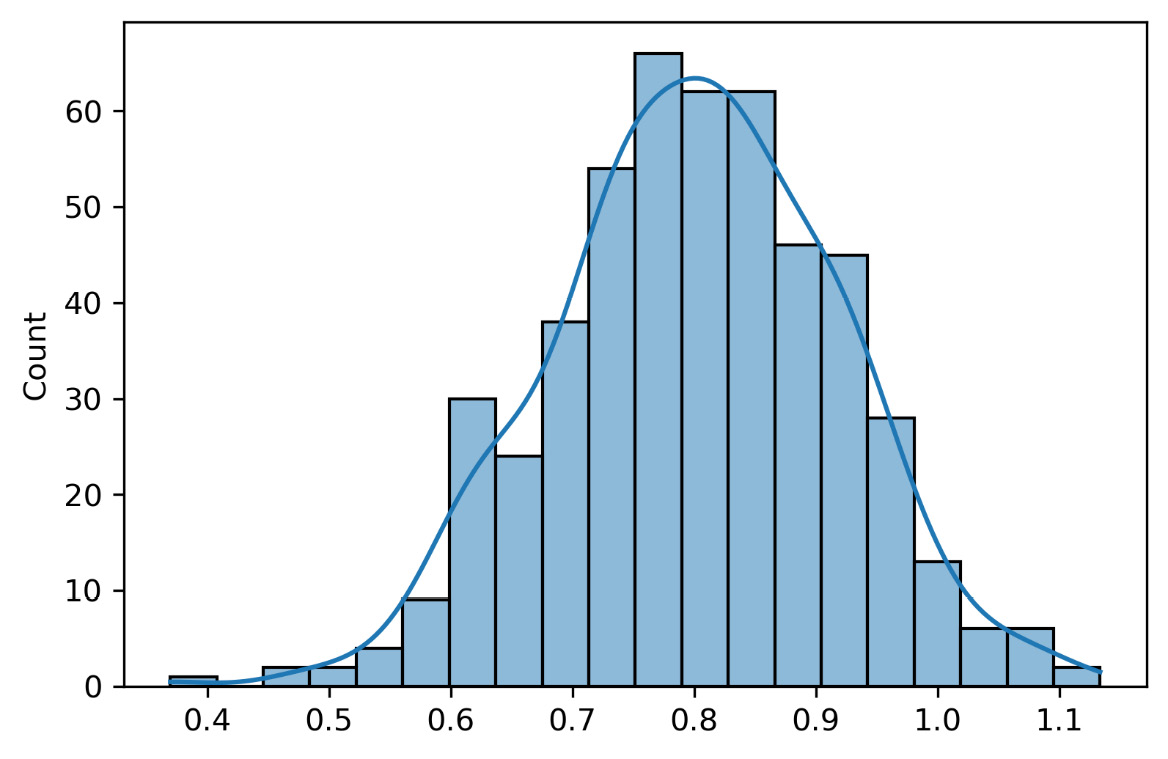
Figure 6.6 – The model’s slope distribution
The following graph shows the distribution of the intercept of all 500 models fitted to the samples extracted from the initial distributions:
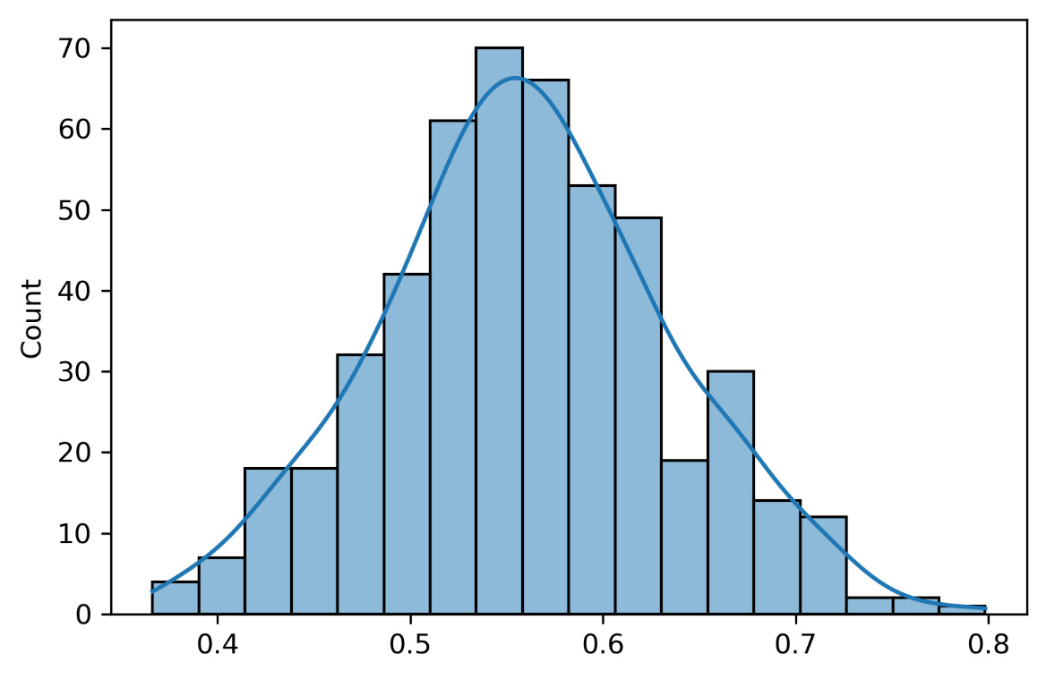
Figure 6.7 – The model’s intercept distribution
- In the final part of this script, we try to evaluate the performance of the 500 models we have worked out in more detail. To start, we will draw a graph with the values of the coefficient of determination r_squared:
plt.plot(r_sqs)
The following graph is returned:

Figure 6.8 – The model’s performance evaluation
We can see that the values oscillate between 0.1 and 0.5, so we try to extract the maximum value:
max_r_sq=max(r_sqs)
print(f"Max R squared = {max_r_sq}")
The following value is displayed:
Max R squared = 0.5245632432772953
If we compare this value with what we obtained with the initial distribution of data (R-squared = 0.286581509708418), the improvement that we’ve obtained is evident. We went from about 28% of the explained variance to 52%. So, we can say that bootstrapping returned a very good result.
Now, let’s try to extract the values of the parameters of the regression line that return these results:
pos_max_r_sq=r_sqs.index(max(r_sqs))
print(f"Boot of the best Regression model = {pos_max_r_sq}")
max_slope=boot_slopes[pos_max_r_sq]
print(f"Slope of the best Regression model = {max_slope}")
max_interc=boot_interc[pos_max_r_sq]
print(f"Intercept of the best Regression model = {max_interc}")
The following results are shown:
Boot of the best Regression model = 383
Slope of the best Regression model = 1.1086506372800053
Intercept of the best Regression model = 0.3752482619581162
In this way, we will be able to draw the regression line that best approximates the resampled data.
Now that we’ve analyzed the resampling techniques in detail, let’s learn how to perform permutation tests.
Explaining permutation tests
When observing a phenomenon belonging to a set of possible results, we ask ourselves what the law of probability is that we can assign to this set. Statistical tests provide a rule that allows us to decide whether to reject a hypothesis based on the sample observations.
Parametric approaches are very uncertain about the experiment plan and the population model. When these assumptions are not respected, particularly when the data law does not conform to the needs of the test, the parametric results are less reliable. When the hypothesis is not based on knowledge of the data distribution and assumptions have not been verified, nonparametric tests are used. Nonparametric tests offer a very important alternative since they need fewer hypotheses.
Permutation tests are a special case of randomization tests that use a series of random numbers formulated from statistical inferences. The computing power of modern computers has made their widespread application possible. These methods do not require that their assumptions about data distribution are met.
A permutation test is performed through the following steps:
- A statistic is defined whose value is proportional to the intensity of the process or relationship being studied.
- A null hypothesis, H0, is defined.
- A dataset is created based on the scrambling of those observed. The mixing mode is defined according to the null hypothesis.
- The reference statistics are recalculated, and the value is compared with the one that was observed.
- The last two steps are repeated many times.
- If the observed statistic is greater than the limit obtained in 95% of the cases based on shuffling, H0 is rejected.
Two experiments use values in the same sample space under the respective distributions, P1 and P2, both of which are members of an unknown population distribution. Given the same dataset, x, if the inference conditional on x, which is obtained using the same test statistic, is the same, assuming that the exchangeability for each group is satisfied in the null hypothesis. The importance of permutation tests lies in their robustness and flexibility. The idea of using these methods is to generate a reference distribution from the data and recalculate the test statistics for each permutation of the data concerning the resulting discrete law.
Now, let’s look at a practical case of a permutation test in a Python environment.
Performing a permutation test
A permutation test is a powerful non-parametric test for comparing the central trends of two independent samples. No verification is needed on the variability of the population groups or the shape of the distribution. The limitation of this test is its application to small samples.
Therefore, the permutation test allows us to evaluate the correlation between the data by returning the distribution of the test statistic under the null hypothesis: it is obtained by calculating all the possible values of the test statistic using an adequate number of resamplings of the observed data. In a dataset, the data labels are associated with those features; if the labels are swapped under the null hypothesis, the resulting tests produce exact significance levels. The confidence intervals can then be derived from the tests.
As mentioned in the Demystifying bootstrapping section, statistical significance tests initially assume the so-called null hypothesis. When comparing two or more groups of data, the null hypothesis always states that there is no difference between the groups regarding the parameter considered: the null hypothesis specifies that the groups are equal to each other and any observed differences must be attributed to chance alone.
We proceed by applying a statistical significance test, the result of which must be compared with a critical value: if the test result exceeds the critical value, then the difference between the groups is declared statistically significant and, therefore, the null hypothesis is rejected; otherwise, the null hypothesis is accepted.
The results of a statistical test do not have a value of absolute and mathematical certainty, but only of probability. Therefore, a decision to reject the null hypothesis is probably right, but it could be wrong. The measure of this risk of falling into error is called the significance level of the test. The significance level of a test can be chosen at will by the researcher, but usually, a probability level of 0.05 or 0.01 is chosen. This probability (called the p-value) represents a quantitative estimate of the probability that the observed differences are due to chance.
The p-value represents the probability of obtaining a more extreme result than the one observed if the diversity is entirely due to the sampling variability alone, thus assuming that the initial null hypothesis is true. p is a probability and therefore can only assume values between 0 and 1. A p-value approaching 0 means a low probability that the observed difference may be due to chance.
Statistically significant does not mean relevant but simply means that what has been observed is hardly due to chance. Numerous statistical tests are used to determine with a certain degree of probability the existence or otherwise of significant differences in the data under examination.
In the example we will analyze, we will compare the data that’s been collected on two observations: the first dataset is the well-known Iris flower dataset. In the second case, we will artificially generate a dataset. Our goal is to verify that, in the first dataset, there is a strong correlation between features and labels, something that is non-existent in the artificially generated dataset.
Here is the Python code (permutation_tests.py). As always, we will analyze the code line by line:
- Let’s start by importing the necessary libraries:
from sklearn.datasets import load_iris
import numpy as np
from sklearn import tree
from sklearn.model_selection import permutation_test_score
import matplotlib.pyplot as plt
import seaborn as sns
The sklearn.datasets library contains the most widely used datasets in data analysis. Among, these we import the well-known Iris dataset. The numpy library is a Python library that contains numerous functions that can help us manage multidimensional matrices. Furthermore, it contains a large collection of high-level mathematical functions we can use on these matrices. Here, we imported the tree classification model from the sklearn library. Then, we imported the permutation_test_score() function from sklearn.model_selection, which calculates the significance of a cross-validated score with permutations. The matplotlib library is a Python library for printing high-quality graphics. Finally, we imported the seaborn library. It is a Python library that enhances the data visualization tools of the matplotlib module. In the seaborn module, there are several features we can use to graphically represent our data. Some methods facilitate the construction of statistical graphs with matplotlib.
- Let’s import the data:
data=data = load_iris()
X = data.data
y = data.target
The Iris dataset is a multivariate dataset introduced by the British statistician and biologist Ronald Fisher in 1936 as an example of linear discriminant analysis. The dataset contains 50 samples from each of the three species of Iris (Iris setosa, Iris virginica, and Iris versicolor). Four features were measured from each sample: the length and the width of the sepals and petals, in centimeters.
The following variables are contained:
- Sepal.Length in centimeters
- Sepal.Width in centimeters
- Petal.Length in centimeters
- Petal.Width in centimeters
- Class: setosa, versicolour, virginica
- Now, let’s create a completely artificial dataset with several features equal to those of the
Iris dataset, but which do not have any correlation with the labels of the Iris dataset:
np.random.seed(0)
X_nc_data = np.random.normal(size=(len(X), 4))
To do this, we used numpy’s random.normal() function. This function generates a normal distribution by default and uses a mean equal to 0 and a standard deviation equal to 1. We added the seed for reproducibility.
- Our goal is to evaluate the correlation in the data by performing a classification of the labels (y) based on the features contained in the matrix, X. Let’s choose the classification model:
clf = tree.DecisionTreeClassifier(random_state=1)
Here, DecisionTreeClassifier was chosen. A decision tree algorithm is based on a non-parametric supervised learning method used for classification and regression. The aim is to build a model that predicts the value of a target variable using decision rules inferred from the data features.
- Now, let’s perform a permutation test on the data:
p_test_iris = permutation_test_score(
clf, X, y, scoring="accuracy", n_permutations=1000
)
print(f"Score of iris flower classification = {p_test_iris[0]}")print(f"P_value of permutation test for iris dataset = {p_test_iris[2]}")p_test_nc_data = permutation_test_score(
clf, X_nc_data, y, scoring="accuracy", n_permutations=1000
)
print(f"Score of no-correletd data classification = {p_test_nc_data[0]}")print(f"P_value of permutation test for no-correletd dataset = {p_test_nc_data[2]}")
For the test, we used the permutation_test_score() function, which evaluates the significance of a cross-validated score with permutations. This function performs a permutation of the target to resample the data and calculate the empirical p-value concerning the null hypothesis, which assumes the characteristics and objectives are independent. Three results are returned:
- score: The score of the real classification without trade-in on the targets
- permutation_scores: Scores obtained for each permutation
- pvalue: Approximate probability that the score is obtained by chance
The p-value represents the fraction of randomized datasets in which the classifier performed well: a small p-value tells us that there is a real dependence between characteristics and targets. A high p-value may be due to a lack of real dependency between characteristics and targets.
- First, we performed the test on the data from the Iris dataset and obtained the following results:
Score of iris flower classification = 0.9666666666666668
P_value of permutation test for iris dataset = 0.000999000999000999
1,000 permutations have been made: the accuracy of the decision tree-based classifier is very high, which tells us that the model can predict the class of the type of Iris with excellent performance. However, the p-value is very low, which confirms the real dependence of the target, y, on the features contained in the matrix, X.
- Then, we ran the same test on the artificially generated data. The following results were returned:
Score of no-correletd data classification = 0.2866666666666667
P_value of permutation test for no-correletd dataset = 0.8711288711288712
The classification score is low, indicating that the forecasts do not have good accuracy. However, the p-value is high, which indicates that a correlation between the features and the target has not been found.
- Finally, we performed a visual analysis of the results of the permutation test:
pbox1=sns.histplot(data=p_test_iris[1], kde=True)
plt.axvline(p_test_iris[0],linestyle="-", color='r')
plt.axvline(p_test_iris[2],linestyle="--", color='b')
pbox1.set(xlim=(0,1))
plt.show()
The following graph was displayed:

Figure 6.9 – Histogram with a density curve for the permutation test
This graph shows a histogram with the density curve of the distribution of the results of the permutation tests performed 100 times. A blue dashed vertical line is drawn to indicate the p-value, and a continuous red vertical line is drawn to indicate the accuracy of the classifier. Note that since these are the original data (Iris dataset), characterized by a strong correlation between features and targets, the score of the classifier is much higher than those obtained by permuting the targets: the permutations of the targets cause the correlation between the features and targets to be lost. Furthermore, the p-value is located on the far left of the graph to indicate a low value and therefore a strong correlation between the features and targets.
Let’s see what happens to the randomly generated data:

Figure 6.10 – Histogram with a density curve for the randomly generated data
In this case, being random data, characterized by no correlation between features and targets, the score of the classifier is low and in line with those obtained by permuting the targets. Furthermore, the p-value is on the far right of the graph to indicate a high value and therefore a low correlation between the features and targets.
Now that we’ve analyzed a practical case of permutation testing, let’s learn how to perform data resampling by applying cross-validation.
Approaching cross-validation techniques
Cross-validation is a method used in model selection procedures based on the principle of predictive accuracy. A sample is divided into two subsets, of which the first (training set) is used for construction and estimation, while the second (validation set) is used to verify the accuracy of the predictions of the estimated model. Through a synthesis of repeated predictions, a measure of the accuracy of the model is obtained. A cross-validation method is like Jackknife in that it leaves one observation out at a time. In another method, known as k-fold validation, the sample is divided into k subsets and, in turn, each of them is left out as a validation set.
Important note
Cross-validation can be used to estimate the mean squared error (MSE) (or, in general, any measure of precision) of a statistical learning technique to evaluate its performance or select its level of flexibility.
Cross-validation can be used for both regression and classification problems. The three main validation techniques of a simulation model are the validation set approach, leave-one-out cross-validation (LOOCV), and k-fold cross-validation. In the following sections, we will learn about these concepts in more detail.
Validation set approach
This technique consists of randomly dividing the available dataset into two parts:
- A training set
- A validation set, called the holdout set
A statistical learning model is adapted to the training data and subsequently used for predicting the data of the validation set.
The measurement of the resulting test error, which is typically the MSE in the case of regression, provides an estimate of the real test error. The validation set is the result of a sampling procedure and therefore different samplings result in different estimates of the test error.
This validation technique has various pros and cons. Let’s take a look at a few:
- The method tends to have high variability; that is, the results can change substantially as the selected test set changes.
- Only a part of the available units is used for function estimates. This can lead to less precision in function estimating and overestimating the test error.
The LOOCV and k-fold cross-validation techniques try to overcome these problems.
Leave-one-out cross-validation
LOOCV also divides the observation set into two parts. However, instead of creating two subsets of comparable size, we do the following:
- A single observation (x1, y1) is used for validation; the remaining observations make up the training set.
- The function is estimated based on the n-1 observations of the training set.
- The prediction,
 , is made using x1. Since (x1, y1) was not used in the function estimate, an estimate of the test error is as follows:

But even if MSE1 is impartial to the test error, it is a poor estimate because it is very variable. This is because it is based on a single observation (x1, y1).
- The procedure is repeated by selecting for validation (x2, y2), where a new estimate of the function is made based on the remaining n-1 observations, and calculating the test error again, as follows:

- Repeating this approach n times produces n test errors.
- The LOOCV estimate for the MSE test is the average of the n MSEs available, as follows:

LOOCV has some advantages over the validation set approach:
- Using an n-1 unit to estimate the function has less bias. Consequently, the LOOCV approach does not tend to overestimate the test error.
- As there is no randomness in the choice of the test set, there is no variability in the results for the same initial dataset.
LOOCV can be computationally intensive, so for large datasets, it takes a long time to calculate. In the case of linear regression, however, there are direct computational formulas with low computational intensity.
k-fold cross-validation
In k-fold cross-validation (k-fold CV), the set of observations is randomly divided into k groups, or folders, of approximately equal size. The first folder is considered a validation set and the function is estimated on the remaining k-1 folders. The mean square error, MSEi, is then calculated on the observations of the folder that’s kept out. This procedure is repeated k times, each time choosing a different folder for validation, thus obtaining k estimates of the test error. The k-fold CV estimate is calculated by averaging these values, as follows:

This method has the advantage of being less computationally intensive if k << n. Furthermore, the k-fold CV tends to have less variability than the LOOCV on different-sized datasets, n.
Choosing k is crucial in k-fold CV. What happens when i changes in cross-validation? Let’s see what an extreme choice of k entails:
- A high k value results in larger training sets and therefore less bias. This implies small validation sets and therefore greater variance.
- A low k value results in smaller training sets and therefore greater bias. This implies larger validation sets and therefore low variance.
Cross-validation using Python
In this section, we will look at an example of the application of cross-validation. First, we will create an example dataset that contains simple data to identify to verify the procedure being performed by the algorithm. Then, we will apply k-fold CV and analyze the results:
- As always, we will start by importing the necessary libraries:
import numpy as np
from sklearn.model_selection import KFold
numpy is a Python library that contains numerous functions that help us manage multidimensional matrices. Furthermore, it contains a large collection of high-level mathematical functions we can use on these matrices.
scikit-learn is an open source Python library that provides multiple tools for machine learning. In particular, it contains numerous classification, regression, and clustering algorithms; this includes support vector machines, logistic regression, and much more. Since it was released in 2007, scikit-learn has become one of the most widely used libraries in the field of machine learning, both supervised and unsupervised, thanks to the wide range of tools it offers, but also thanks to its API, which is documented, easy to use, and versatile.
Important note
Application programming interfaces (APIs) are sets of definitions and protocols that application software is created and integrated with. They allow products or services to communicate with other products or services without knowing how they are implemented, thus simplifying app development, and allowing a net saving of time and money. When creating new tools and products or managing existing ones, APIs offer flexibility, simplify design, administration, and use, and provide opportunities for innovation.
The scikit-learn API combines a functional user interface with an optimized implementation of numerous classification and meta-classification algorithms. It also provides a wide variety of data pre-processing, cross-validation, optimization, and model evaluation functions. scikit-learn is particularly popular for academic research since developers can use the tool to experiment with different algorithms by changing only a few lines of code.
Here, we generated a vector containing 10 integers, starting from the value 10 up to 100 with a step equal to 10. To do this, we used the numpy arange() function. This function generates equidistant values within a certain range. Three arguments have been passed, as follows:
- 10: Start of the interval. This value is included. If this value is omitted, the default value of 0 is used.
- 110: End of range. This value is not included in the range except in cases of floating-point numbers.
- 10: Spacing between values. This is the distance between two adjacent values. By default, this value is equal to 1.
The following array was returned:
[ 10 20 30 40 50 60 70 80 90 100]
- Now, we can set the function that will allow us to perform k-fold CV:
kfold = KFold(5, True, 1)
scikit-learn’s KFold() function performs k-fold CV by dividing the dataset into k consecutive folds without shuffling by default. Each fold is then used once as validation, while the remaining k - 1 folds form the training set. Three arguments were passed, as follows:
- 5: Number of folds required. This number must be at least 2.
- True: Optional Boolean value. If it is equal to True, the data is mixed before it’s divided into batches.
- 1: Seed used by the random number generator.
- Finally, we can resample the data by using k-fold CV:
for TrainData, TestData in kfold.split(StartedData):
print("Train Data :", StartedData[TrainData],"Test Data :", StartedData[TestData])
To do this, we used a loop for the elements generated by the kfold.split() method, which returns the indexes that the dataset is divided into. Then, for each step, which is equal to the number of folds, the elements of the subsets that were drawn are printed.
The following results are returned:
Train Data : [ 10  20  40  50  60  70  80  90]
Test Data : [ 30 100]
Train Data : [ 10  20  30  40  60  80  90 100]
Test Data : [50 70]
Train Data : [ 20  30  50  60  70  80  90 100]
Test Data : [10 40]
Train Data : [ 10  30  40  50  60  70  90 100]
Test Data : [20 80]
Train Data : [ 10  20  30  40  50  70  80 100]
Test Data : [60 90]
These pairs of data (Train Data, Test Data) will be used in succession to train the model and validate it. This way, you can avoid overfitting and bias problems. Every time you evaluate the model, the extracted part of the dataset is used, and the remaining part of the dataset is used for training.
Summary
In this chapter, we learned how to resample a dataset. We analyzed several techniques that approach this problem through different techniques. First, we analyzed the basic concepts of sampling and learned about the reasons that push us to use a sample extracted from a population. Then, we examined the pros and cons of this choice. We also analyzed how a resampling algorithm works.
Then, we tackled the first resampling method: the Jackknife method. First, we defined the concepts behind the method and then moved on to the procedure, which allows us to obtain samples from the original population. To put the concepts we learned into practice, we applied Jackknife resampling to a practical case.
Next, we explored the bootstrap method, which builds unobserved but statistically, like the observed samples. This is accomplished by resampling the observed series through an extraction procedure where we reinsert the observations. After defining the method, we worked through an example to highlight the characteristics of the procedure. Furthermore, a comparison between Jackknife and bootstrap was made. Then, we analyzed a practical case of bootstrapping applied to a regression problem.
After analyzing the concepts underlying permutation tests and exploring an example of this test, we concluded this chapter by looking at various cross-validation methods. Our knowledge of the k-fold CV method was deepened through an example.
In the next chapter, we will learn about the basic concepts of various optimization techniques and how to implement them. We will understand the difference between numerical and stochastic optimization techniques, and we will learn how to implement stochastic gradient descent. Then, we will discover how to estimate missing or latent variables and optimize model parameters. Finally, we will discover how to use optimization methods in real-life applications.