9

Using Simulation Models for Financial Engineering

The massive use of systems based on artificial intelligence and machine learning has opened up new scenarios for the financial sector. These methods can increase benefits, not only, for example, by protecting user rights but also in terms of macroeconomics.

Monte Carlo methods find a natural application in finance for the numerical resolution of pricing and option coverage problems. Essentially, these methods consist of simulating a given process or phenomenon using a given mathematical law and a sufficiently large set of data, created randomly from distributions that adequately represent real variables. The idea is that, if an analytical study is not possible, or adequate experimental sampling is not possible or convenient, the numerical simulation of the phenomenon is used. In this chapter, we will look at practical cases of using simulation methods in a financial context. You will learn how to use Monte Carlo methods to predict stock prices and how to assess the risk associated with a portfolio of shares.

In this chapter, we’re going to cover the following topics:

• Understanding the geometric Brownian motion model
• Using Monte Carlo methods for stock price prediction
• Studying risk models for portfolio management

Technical requirements

In this chapter, we will learn how to use simulation models for financial engineering. In order to understand these topics, a basic knowledge of algebra and mathematical modeling is needed.

To work with the Python code in this chapter, you need the following files (available on GitHub at https://github.com/PacktPublishing/Hands-On-Simulation-Modeling-with-Python-Second-Edition):

• standard_brownian_motion.py
• amazon_stock_montecarlo_simulation.py
• value_at_risk.py

Understanding the geometric Brownian motion model

The name Brownian comes from the Scottish botanist Robert Brown who, in 1827, observed, under the microscope, how pollen particles suspended in water moved continuously in a random and unpredictable way. In 1905, it was Einstein who gave a molecular interpretation of the phenomenon of movement observed by Brown. He suggested that the motion of the particles was mathematically describable, assuming that the various jumps were due to the random collisions of pollen particles with water molecules.

Today, Brownian motion is, above all, a mathematical tool in the context of probability theory. This mathematical theory has been used to describe an ever-widening set of phenomena, studied by disciplines that are very different from physics. For instance, the prices of financial securities, the spread of heat, animal populations, bacteria, illness, sound, and light are modeled using the same theory.

Important note

Brownian motion is a phenomenon that consists of the uninterrupted and irregular movement made by small particles or grains of colloidal size – that is, particles that are far too small to be observed with the naked eye but are significantly larger than atoms when immersed in a fluid.

Defining a standard Brownian motion

There are various ways of constructing a Brownian motion model and various equivalent definitions of Brownian motion. Let’s start with the definition of a standard Brownian motion (the Wiener process). The essential properties of the standard Brownian motion include the following:

1. The standard Brownian motion starts from zero.
2. The standard Brownian motion takes a continuous path.
3. The change in motion from the previous step (the increments suffer) by the Brownian process is independent.
4. The increases suffered by the Brownian process in the time interval, dt, indicate a Gaussian distribution, with an average that is equal to zero and a variance that is equal to the time interval, dt.

Based on these properties, we can consider the process as the sum of an unlimited large number of extremely small increments. After choosing two instants, t and s, the random variable, Y(s) -Y(t), follows a normal distribution, with a mean of (s-t) and variance of (s-t), which we can represent using the following equation:

The hypothesis of normality is very important in the context of linear transformations. In fact, the standard Brownian motion takes its name from the standard normal distribution type, with parameters of = 0 and = 1.

Therefore, it can be said that the Brownian motion, Y (t), with a unit mean and variance can be represented as a linear transformation of a standard Brownian motion, according to the following equation:

In the previous equation, we can see that is the standard Brownian motion.

The weak point of this equation lies in the fact that the probability that Y (t) assumes a negative value is positive; in fact, since Z (t) is characterized by independent increments, which can assume a negative sign, the risk of the negativity of Y (t) is not zero.

Now, let’s consider the standard Brownian motion (the Wiener process) for sufficiently small time intervals. An infinitesimal increment of this process is obtained in the following form:

Here, N is the number of samples. The previous equation can be rewritten as follows:

This process is not limited in variation and, therefore, cannot be differentiated in the context of classical analysis. In fact, the previous one tends to infinity or tends to zero of the interval, dt.

Addressing the Wiener process as random walk

A Wiener process can be considered a borderline case of random walk. We dealt with random walk in Chapter 5, Simulation-Based Markov Decision Processes. We have seen that the position of a particle at instant n will be represented by the following equation:

In the previous formula, we can observe the following:

• Yn is the next value in the walk
• Yn-1 is the observation in the previous time phase
• Zn is the random fluctuation in that step

If the n random numbers, Zn, have a mean equal to zero and a variance equal to 1, then, for each value of n, we can define a stochastic process using the following equation:

The preceding formula can be used in an iterative process. For very large values of n, we can write the following:

The previous formula is due to the central limit theorem that we covered in Chapter 4, Exploring Monte Carlo Simulations.

Implementing a standard Brownian motion

So, let’s demonstrate how to generate a simple Brownian motion in the Python environment. Let’s start with the simplest case, in which we define the time interval, the number of steps to be performed, and the standard deviation:

1. We start by importing the following libraries:

   import numpy as np

   import matplotlib.pyplot as plt

The numpy library is a Python library containing numerous functions that can help us in the management of multidimensional matrices. Additionally, it contains a large collection of high-level mathematical functions that we can use to operate on these matrices.

The matplotlib library is a Python library used for printing high-quality graphics. With matplotlib, it is possible to generate graphs, histograms, bar graphs, power spectra, error graphs, scatter graphs, and more using just a few commands. This includes a collection of command-line functions similar to those provided by MATLAB software.

2. Now, let’s proceed with some initial settings:

   np.random.seed(4)

   n = 1000

   sqn = 1/np.math.sqrt(n)

   z_values = np.random.randn(n)

   Yk = 0

   sb_motion=list()

In the first line of code, we used the random.seed() function to initialize the seed of the random number generator. This way, the simulation that uses a random number generator will be reproducible. The reproducibility of the experiment is possible because the randomly generated numbers are always the same. We set the number of iterations (n), and we calculated the first term of the following equation:

Then, we generated the n random numbers using the random.randn() function. This function returns a standard normal distribution of n samples with a mean of 0 and a variance of 1. Finally, we set the first value of the Brownian motion as required from the properties, (Y(0)=0), and we initialized the list that will contain the Brownian motion positions.

3. At this point, we will use a for loop to calculate all of the n positions:

   for k in range(n):

       Yk = Yk + sqn*z_values[k]

       sb_motion.append(Yk)

We simply added the current random number, multiplied by sqn, to the variable that contains the cumulative sum. The current value is then appended to the SBMotion list.

4. Finally, we draw a graph of the Brownian motion created:

   plt.plot(sb_motion)

   plt.show()

The following plot is printed:

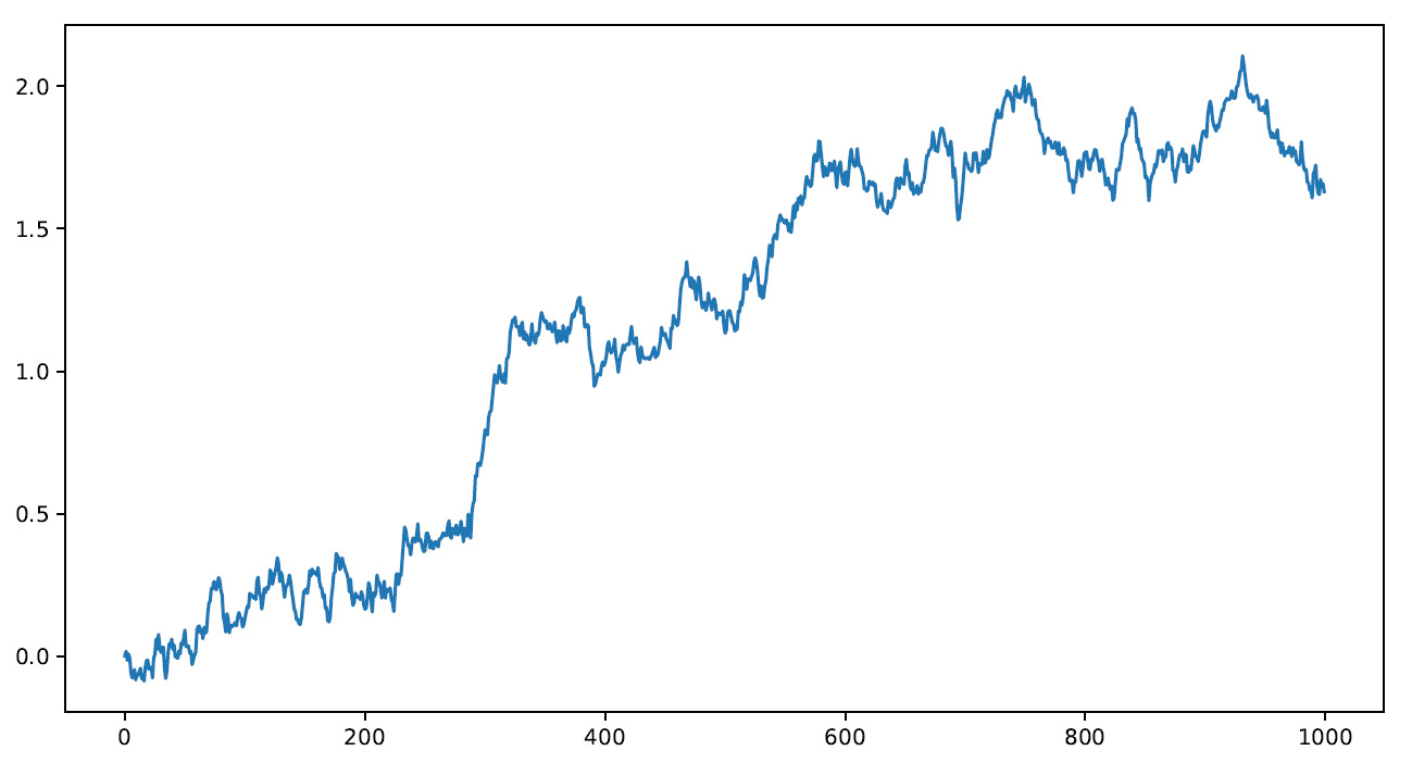
Figure 9.1 – A Brownian motion graph

So, we have created our first simulation of Brownian motion. Its use is particularly suitable for financial simulations. In the next section, we will demonstrate how this is done using a Monte Carlo simulation.

Using Monte Carlo methods for stock price prediction

As we explored in Chapter 4, Exploring Monte Carlo Simulations, Monte Carlo methods simulate different evolutions of the process under examination, using different probabilities that an event may occur under certain conditions. These simulations explore the entire parameter space of the phenomenon and return a representative sample. For each sample obtained, measures of the quantities of interest are carried out to evaluate their performance. A correct simulation means that the average value of the result of the process converges to the expected value.

Exploring the Amazon stock price trend

The stock market provides an opportunity to quickly earn large amounts of money – that is, in the eyes of an inexperienced user at least. Exchanges on the stock market make really large amounts, attracting in turn the attention of speculators from all over the world. In order to obtain revenues from investments in the stock market, it is necessary to have solid knowledge obtained from years of in-depth study of the phenomenon. In this context, the possibility of having a tool to predict stock market securities represents a popular need.

Let’s demonstrate how to develop a simulation model of the stock of one of the most famous companies in the world. Amazon was founded by Jeff Bezos in the 1990s, and it was one of the first companies in the world to sell products via the internet. Amazon stock has been listed on the stock exchange since 1997 under the symbol AMZN. The historical values of AMZN stock can be obtained from various internet sites that have been dealing with the stock market over the past 10 years. We will refer to the performance of AMZN stock on the NASDAQ GS stock quote from 2012-10-03 to 2022-09-30. To select this date range, simply click on the Time Period item and select it.

Data can be downloaded in the .csv format from the Yahoo Finance website at https://finance.yahoo.com/quote/AMZN/history/.

In the following screenshot, you can see the Yahoo Finance section for AMZN stock with a highlighted button to download the data:

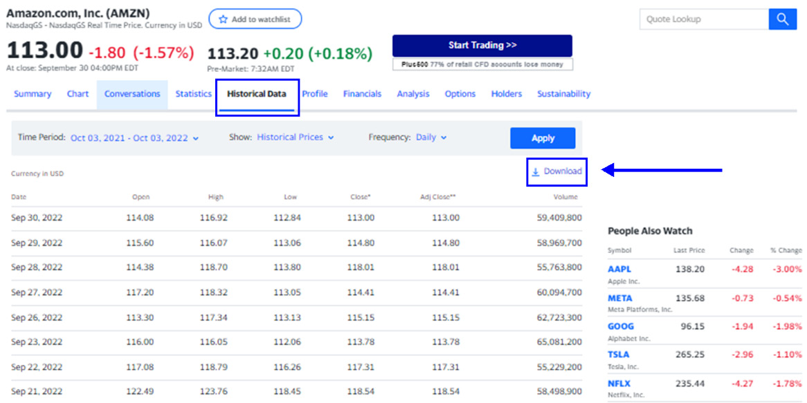
Figure 9.2 – Amazon data on Yahoo Finance

The downloaded AMZN.csv file contains a lot of features, but we will only use two of them, as follows:

• Date: The date of the quote
• Close: The close price

We will analyze the code, line by line, to fully understand the whole process that will lead us to simulate a series of predictions of Amazon stock price performance:

1. As always, we start by importing the libraries:

   import numpy as np

   import pandas as pd

   import matplotlib.pyplot as plt

   from scipy.stats import norm

   from pandas.plotting import 

              register_matplotlib_converters

The following libraries were imported:

• The numpy library is a Python library that contains numerous functions to help us in the management of multidimensional matrices. Furthermore, it contains a large collection of high-level mathematical functions to operate on these matrices.
• The pandas library is an open source BSD-licensed library that contains data structures and operations to manipulate high-performance numeric values for the Python programming language.
• The matplotlib library is a Python library used for printing high-quality graphics. With matplotlib, it is possible to generate graphs, histograms, bar graphs, power spectra, error graphs, scatter graphs, and more with just a few commands. This includes a collection of command-line functions such as those provided by MATLAB software.
• SciPy is a collection of mathematical algorithms and functions based on NumPy. It has a series of commands and high-level classes to manipulate and display data. With SciPy, functionality is added to Python, making it a data processing and system prototyping environment similar to commercial systems such as MATLAB.

The pandas.plotting.register_matplotlib_converters() function makes pandas formatters and converters compatible in matplotlib. Let’s use it now:

register_matplotlib_converters()

2. Now, let’s import the data contained in the AMZN.csv file:

   AmznData = pd.read_csv('AMZN.csv',header=0, 

              usecols = ['Date',Close'],parse_dates=True,

              index_col='Date')

We used the read_csv module of the pandas library, which loads the data in a pandas object called DataFrame. The following arguments are passed:

• 'AMZN.csv': The name of the file.
• header=0: The row number containing the column names and the start of the data. By default, if a non-header row is passed (header=0), the column names are inferred from the first line of the file.
• usecols=['Date',Close']: This argument extracts a subset of the dataset by specifying the column names.
• parse_dates=True: A Boolean value; if True, try parsing the index.
• index_col='Date': This allows us to specify the name of the column that will be used as the index of the DataFrame.

3. Now, we will explore the imported dataset to extract preliminary information. To do this, we will use the info() function, as follows:

   print(AmznData.info())

The following information is printed:

<class 'pandas.core.frame.DataFrame'>
DatetimeIndex: 2515 entries, 2012-10-03 to 2022-09-30
Data columns (total 1 columns):
 #   Column  Non-Null Count  Dtype  
---  ------  --------------  -----  
 0   Close   2515 non-null   float64
dtypes: float64(1)
memory usage: 39.3 KB
None

Here, a lot of useful information is returned: the object class, the number of records present (2,515), the start and end values of the index (2012-10-03 to 2022-09-30), the number of columns and the type of data they contain, and other information.

We can also print the first five lines of the dataset, as follows:

print(AmznData.head())

The following data is printed:

                 Close
              Close
Date               
2012-10-03  12.7960
2012-10-04  13.0235
2012-10-05  12.9255
2012-10-08  12.9530
2012-10-09  12.5480

If we wanted to print a different number of records, it would be enough to specify it by indicating the number of lines to be printed. Similarly, we can print the last 10 records of the dataset:

print(AmznData.tail())

The following records are printed:

                  Close
Date                   
2022-09-26  115.150002
2022-09-27  114.410004
2022-09-28  118.010002
2022-09-29  114.800003
2022-09-30  113.000000

An initial quick comparison between the head and the tail allows us to verify that Amazon stock in the last 10 years has gone from a value of about $12.79 to about $113.00. This is an excellent deal for Amazon shareholders.

Using the describe() function, we will extract a preview of the data using basic statistics:

print(AmznData.describe())

The following results are returned:

             Close
count  2515.000000
mean     71.683993
std      53.944668
min      11.030000
25%      19.921750
50%      50.187000
75%     104.449249
max     186.570496

We can confirm the significant increase in value in the last 10 years, but we can also see how the stock has undergone significant fluctuations, given the very high value of the standard deviation. This tells us that the shareholders who were loyal to the share and maintained it over time benefited the most from its increase.

4. After analyzing the preliminary data statistics, we can take a look at the performance of Amazon’s share in the last 10 years by drawing a simple graph:

   plt.figure(figsize=(10,5))

   plt.plot(AmznData)

   plt.show()

The following matplotlib functions were used:

• figure(): This function creates a new figure, which is empty for now. We set the size of the frame using the figsize parameter, which sets the width and height in inches.
• plot(): This function plots the AmznData dataset.
• show(): This function, when running in iPython in PyLab mode, displays all the figures and returns to the iPython prompt.

The following diagram is printed:

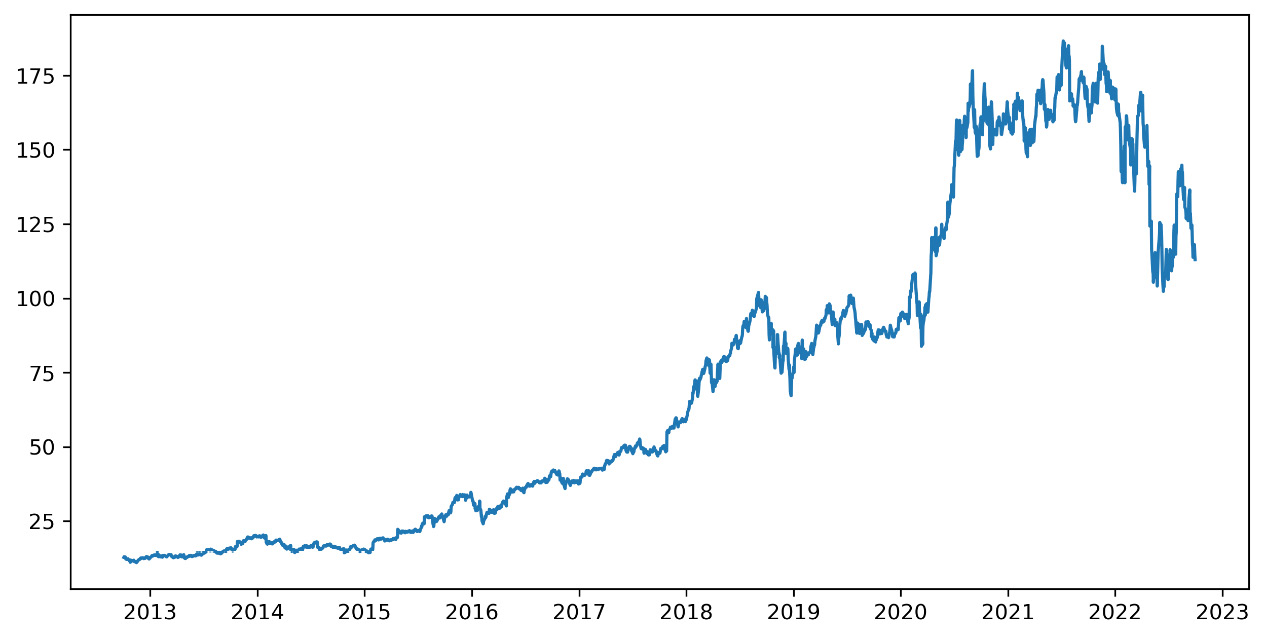
Figure 9.3 – An Amazon share graph

Now it is much clearer, and the significant increase undergone by Amazon stock over the past 10 years is evident. Furthermore, it should be noted that the greatest increase has been recorded since 2015, but we will try to extract more information from the data. We can also see that in the period of the COVID-19 pandemic, there was a further and considerable increase in prices, essentially due to the fact that Amazon was a store accessible to everyone, even during the lockdown period. A significant decrease can also be noted at the beginning of 2022, due to the problems of the war in Ukraine and the increase in energy costs.

Handling the stock price trend as a time series

The trend over time of the Amazon stock price, represented in the previous diagram, is configured as a sequence of ordered data. This type of data can be conveniently handled as a time series. Let’s consider a simple definition: a time series contains a chronological sequence of experimental observations of a variable. This variable can relate to data of different origins. Very often, it concerns financial data such as unemployment rates, spreads, stock market indices, and stock price trends.

The usefulness of dealing with the problem as a time series will allow us to extract useful information from the data in order to develop predictive models for the management of future scenarios. It may be useful to compare the trend of stock prices in the same periods for different years or, more simply, between contiguous periods.

Let’s use Y1, ..., Yt, ..., and Yn as the elements of a time series. Let’s start by comparing the data for two different times, indicated with t and t + 1. It is, therefore, two contiguous periods. We are interested in evaluating the variation undergone by the phenomenon under observation, which can be defined by the following ratio:

This percentage ratio is called a percentage change. It can be defined as the percentage change rate of Y of t + 1 time compared to the previous time, t. This descriptor returns information about how the data underwent a change over a period. The percentage change allows you to monitor both the stock prices and the market indices, not just compare currencies from different countries:

1. To evaluate this useful descriptor, we will use the pct_change() function contained in the pandas library:

   AmznDataPctChange = AmznData.pct_change()

This function returns the percentage change between the current element and a previous element. By default, the function calculates the percentage change from the immediately preceding row.

The concept of the percentage variation of a time series is linked to the concept of the return of a stock price. The returns-based approach allows for the normalization of data, which is an operation of fundamental importance when evaluating the relationships between variables characterized by different metrics.

We will deal with the return on a logarithmic scale, as this choice will give us several advantages: normally distributed results, values returned (the logarithm of the return) very close to the initial return value (at least for very small values), and additive results over time.

2. To pass the return on a logarithmic scale, we will use the log() function of the numpy library, as follows:

   AmznLogReturns = np.log(1 + AmznDataPctChange) 

   print(AmznLogReturns.tail(10))

The following results are printed:

               Close
Date                
2022-09-19  0.009106
2022-09-20 -0.020013
2022-09-21 -0.030327
2022-09-22 -0.010430
2022-09-23 -0.030553
2022-09-26  0.011969
2022-09-27 -0.006447
2022-09-28  0.030981
2022-09-29 -0.027578
2022-09-30 -0.015804

3. To better understand how the return is distributed over time, let’s draw a diagram:

   plt.figure(figsize=(10,5))

   plt.plot(AmznLogReturns)

   plt.show()

The following diagram is printed:

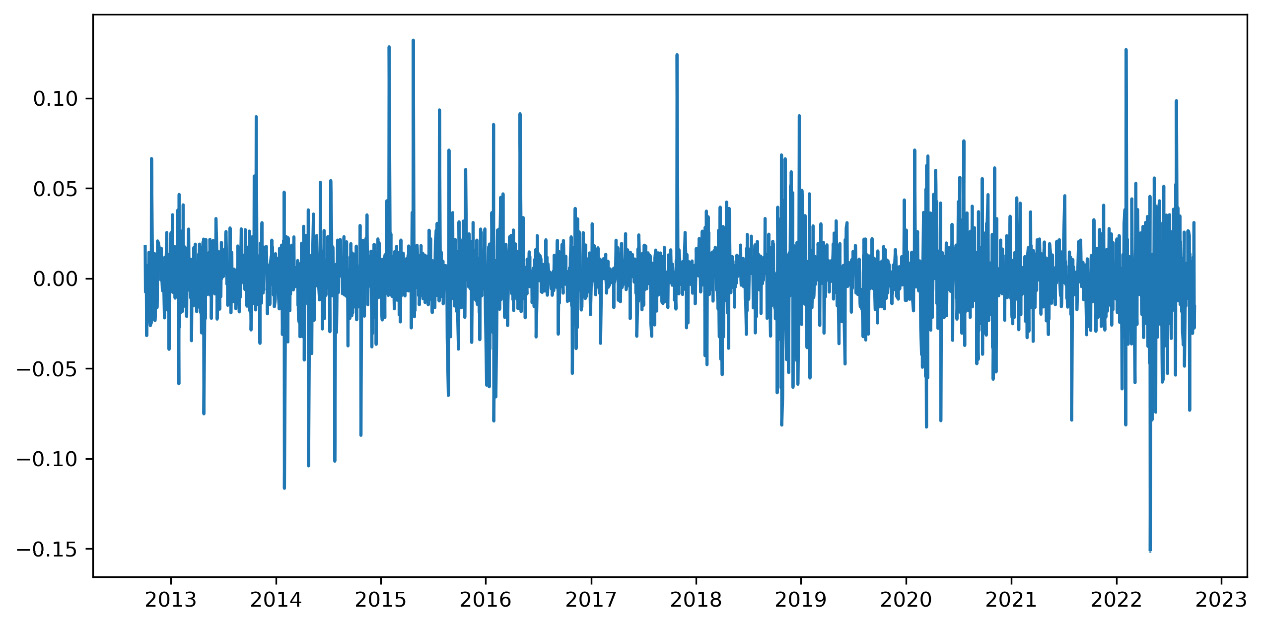
Figure 9.4 – The logarithmic values of the returns

The previous diagram shows us that the logarithmic return is normally distributed over the entire period and the mean is stable.

Introducing the Black-Scholes model

The Black-Scholes (BS) model certainly represents the most important and revolutionary work in the history of quantitative finance. In traditional financial literature, it is assumed that almost all financial asset prices (stocks, currencies, and interest rates) are driven by a Brownian drift motion.

This model assumes that the expected return of an asset is equal to the non-risky interest rate, r. This approach is capable of simulating returns on a logarithmic scale of an asset. Suppose we observe an asset in the instants: t (0), t (1) ,. . , and t (n). We denote, using s (i) = S (ti), the value of an asset at t(i). Based on these hypotheses, we can calculate the return using the following equation:

Then, we will transform the return on the logarithmic scale, as follows:

By applying the BS approach to Brownian geometric motion, the stock price will satisfy the following stochastic differential equation:

In the previous equation, dB(t) is a standard Brownian motion and μ and σ are real constants. The previous equation is valid in the hypothesis that s (i) - s (i - 1) is small, and this happens when the stock prices undergo slight variations. This is because ln (1 + z) is roughly equal to z if z is small. The analytical solution of the previous equation is the following equation:

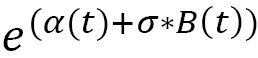
By passing the previous equation on a logarithmic scale, we obtain the following equation:

In the previous equation, we can observe the following:

• α is the drift
• B(t) is a standard Brownian motion
• is the standard deviation

We introduced the concept of drift, which represents the trend of a long-term asset in the stock market. To understand drift, we will use an analogy of river currents. If we pour liquid color into a river, it will spread by following the direction imposed by the river current. Similarly, drift represents the tendency of a stock to follow the trend of a long-term asset.

Applying the Monte Carlo simulation

Using the BS model discussed in the previous section, we can evaluate the daily price of an asset starting from that of the previous day, multiplied by an exponential contribution based on a coefficient, r. This coefficient is a periodic rate of return. It translates into the following equation:

The second term in the previous equation, er, is called the daily return, and according to the BS model, it is given by the following formula:

There is no way to predict the rate of return of an asset. The only way to represent it is to consider it as a random number. So, to predict the price trend of an asset, we can use a model based on random movement such as that represented by BS equations.

The BS model assumes that changes in the stock price depend on the expected return over time. The daily return has two terms: the fixed drift rate and the random stochastic variable. The two terms provide for the certainty of movement and uncertainty caused by volatility.

To calculate the drift, we will use the expected rate of return, which is the most likely rate to occur, using the historical average of the log returns and variance, as follows:

According to the previous equation, the daily change rate of the asset is the mean of the returns, which are less than half of the variance over time. Let’s continue our work, calculating the drift for the return of the Amazon security calculated in the Handling the stock price trend as time series section:

1. To evaluate the drift, we need the mean and variance of the returns. Since we are also calculating the standard deviation, we will need the calculation of the daily return:

   MeanLogReturns = np.array(AmznLogReturns.mean())

   VarLogReturns = np.array(AmznLogReturns.var()) 

   StdevLogReturns = np.array(AmznLogReturns.std())

Three numpy functions were used:

• mean(): This computes the arithmetic mean along the specified axis and returns the average of the array elements.
• var(): This computes the variance along the specified axis. It returns the variance of the array elements, which is a measure of the spread of a distribution.
• std(): This computes the standard deviation along the specified axis.

Now, we can calculate the drift as follows:

Drift = MeanLogReturns - (0.5 * VarLogReturns)
print("Drift = ",Drift)

The following result is returned:

Drift =  [0.0006643]

This is the fixed part of the Brownian motion. The drift returns the annualized change in the expected value and compensates for the asymmetry in the results compared to the straight Brownian motion.

2. To evaluate the second component of the Brownian motion, we will use the random stochastic variable. This corresponds to the distance between the mean and the events, expressed as the number of standard deviations. Before doing this, we need to set the number of intervals and iterations. The number of intervals will be equal to the number of observations, which is 2,515, while the number of iterations that represents the number of simulation models that we intend to develop is 20:

   NumIntervals = 2515

   Iterations = 20
3. Before generating random values, it is recommended that you set the seed to make the experiment reproducible:

   np.random.seed(7)

Now, we can generate the random distribution:

SBMotion = norm.ppf(np.random.rand(NumIntervals, Iterations))

A 2515 x 20 matrix is returned, containing the random contribution for the 20 simulations that we want to perform and for the 2,515 time intervals that we want to consider. Recall that these intervals correspond to the daily prices of the last 10 years.

Two functions were used:

• norm.ppf(): This SciPy function gives the value of the variate for which the cumulative probability has the given value.
• np.random.rand(): This NumPy function computes random values in a given shape. It creates an array of the given shape and populates it with random samples from a uniform distribution over [0, 1].

We will calculate the daily return as follows:

DailyReturns = np.exp(Drift + StdevLogReturns * SBMotion)

The daily return is a measure of the change that occurred in a stock’s price. It is expressed as a percentage of the previous day’s closing price. A positive return means the stock has grown in value, while a negative return means it has lost value. The np.exp() function was used to calculate the exponential value of all elements in the input array.

4. After a long preparation, we have arrived at a crucial moment. We will be able to carry out predictions based on the Monte Carlo method. The first thing to do is to recover the starting point of our simulation. Since we want to predict the trend of Amazon stock prices, we recover the first value present in the AMZN.csv file:

   StartStockPrices = AmznData.iloc[0]

The pandas iloc() function is used to return a pure integer using location-based indexing for selection. Then, we will initialize the array that will contain the predictions:

StockPrice = np.zeros_like(DailyReturns)

The NumPy zeros_like() function is used to return an array of zeros with the same shape and type as a given array. Now, we will set the starting value of the StockPrice array, as follows:

StockPrice[0] = StartStockPrices

5. To update the predictions of Amazon stock prices, we will use a for loop that iterates for a number that is equal to the time intervals we are considering:

   for t in range(1, NumIntervals):

       StockPrice[t] = StockPrice[t - 1] * DailyReturns[t]

For the update, we will use the BS model according to the following equation:

Finally, we can view the results:

plt.figure(figsize=(10,5))
plt.plot(StockPrice)   
AMZNTrend = np.array(AmznData.iloc[:, 0:1])
plt.plot(AMZNTrend,'k*')   
plt.show()

The following diagram is printed:

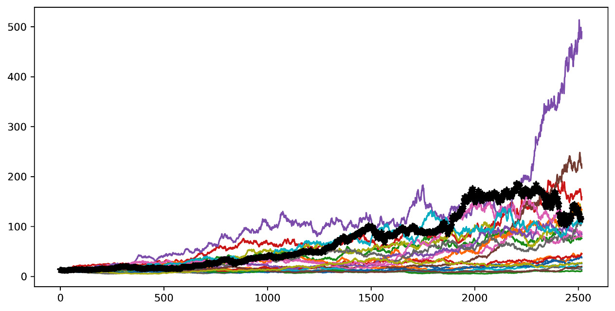
Figure 9.5 – An Amazon trend graph

In the previous diagram, the curve highlighted in black represents the trend of Amazon stock prices in the last 10 years. The other curves are our simulations. We can see that some curves move away from the expected curve, while others appear much closer to the actual trend.

Monte Carlo methods concern the use of random sampling techniques and computer simulation to obtain an approximate solution to a mathematical or financial problem. In other words, we can consider them a family of simulation methods through which it is possible to reproduce and study empirical systems in a controlled form. In practice, these are processes in which data is generated based on a model specified a priori. In this case, we generated data based on the performance of Amazon shares, starting from the prices in the previous period, and then we generated data starting from other data. These methods have now become an integral part of the standard techniques used in statistical methods.

After having seen how it is possible to predict the performance of stock, let’s move on to study how to develop a risk model to manage financial portfolios.

Studying risk models for portfolio management

Having a good risk measure is of fundamental importance in finance, as it is one of the main tools for evaluating financial assets. This is because it allows you to monitor securities and provides a criterion for the construction of portfolios. One measure that has been widely used over the years more than any other is variance.

Using variance as a risk measure

The advantage of a diversified portfolio in terms of risk and expected value is that it allows us to find the right allocation for securities. Our aim is to obtain the highest expected value at the same risk or to minimize the risk of obtaining the same expected value. To achieve this, it is necessary to trace the concept of risk back to a measurable quantity, which is generally referred to as the variance. Therefore, by maximizing the expected value of the portfolio returns for each level of variance, it is possible to reconstruct a curve called the efficient frontier, which determines the maximum expected value that can be obtained with the securities available for the construction of the portfolio for each level of risk.

The minimum variance portfolio represents the portfolio with the lowest possible variance value, regardless of the expected value. This parameter has the purpose of optimizing the risk represented by the variance of the portfolio. Tracing the risk exclusively to the measure of variance is optimal only if the distribution of returns is normal. In fact, the normal distribution enjoys some properties that make the variance a measure that is enough to represent the risk. It is completely determinable through only two parameters (mean and variance). It is, therefore, enough to know the mean and the variance to determine any other point of the distribution.

Introducing the Value-at-Risk metric

Consider the variance as the only risk measure in the case of non-normal and limiting values. A risk measure that has been widely used for over two decades is Value at Risk (VaR). The birth of VaR is linked to the growing need for financial institutions to manage risk and, therefore, to be able to measure it. This is due to the increasingly complex structure of financial markets.

Actually, this measure was not introduced to stem the limits of variance as a risk measure, since an approach to calculate the VaR value starts precisely from the assumptions of normality. However, to make it easier to understand, let’s enclose the overall risk of security into a single number or a portfolio of financial assets by adopting a single metric for different types of risk.

In a financial context, VaR is an estimate, given a confidence interval, of how high the losses of a security or portfolio may be in each time horizon. VaR, therefore, focuses on the left tail of the distribution of returns, where events with a low probability of realization are located. Indicating the losses and not the dispersion of the returns around their expected value makes it a measure closer to the common idea of risk than of variance.

Important note

J.P. Morgan is credited as the bank that made VaR a widespread measure. In 1990, the president of J.P. Morgan, Dennis Weatherstone, was dissatisfied with the lengthy risk analysis reports he received every day. He wanted a simple report that summarized the bank’s total exposure across its entire trading portfolio.

After calculating VaR, we can say that, with a probability given by the confidence interval, we will not lose more than the VaR of the portfolio in the next N days. VaR is the level of loss that will not be exceeded with a probability given by the confidence interval.

For example, a VaR of €1 million over a year with a 95% confidence level means that the maximum loss for the portfolio for the next year will be €1 million in 95% of cases. Nothing tells us what happens to the remaining 5% of cases.

The following diagram shows the probability distribution of portfolio returns with the indication of the value of VaR:

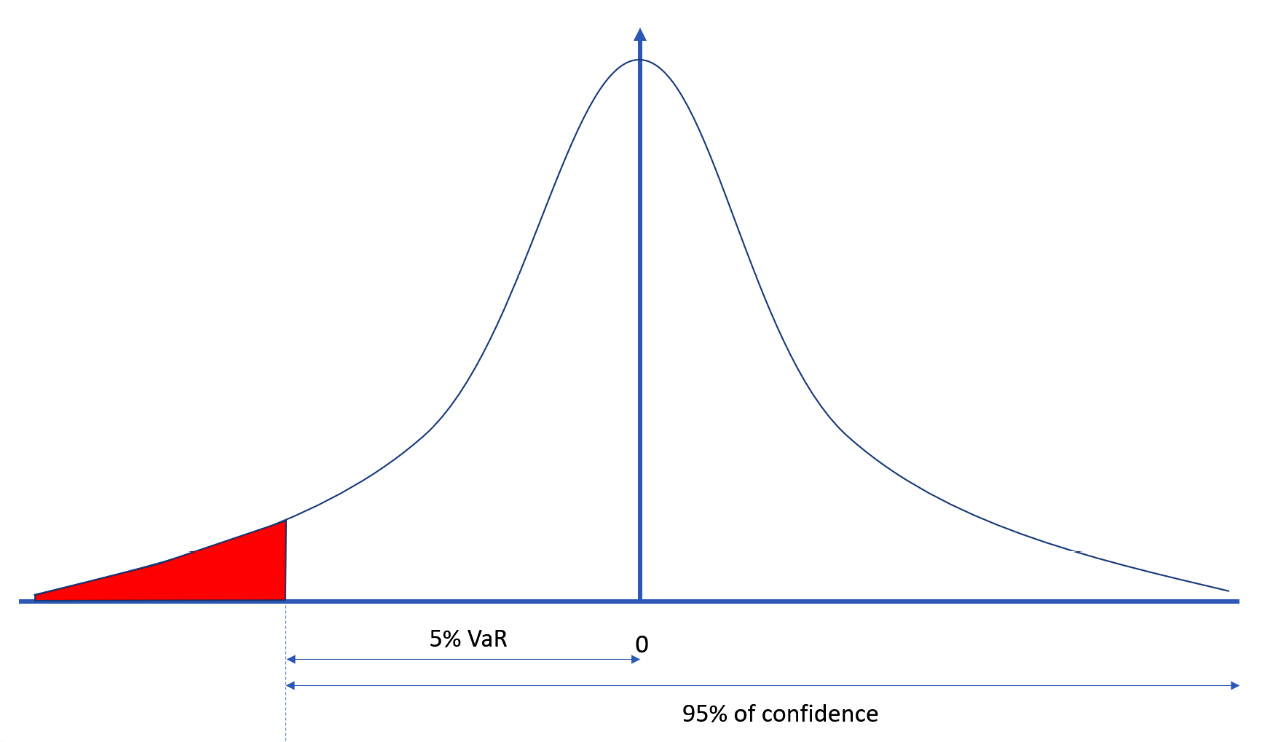
Figure 9.6 – The probability distribution of the portfolio returns

VaR is a function of the following two parameters:

• Time horizon
• Level of confidence

Some characteristics of the VaR must be specified:

• VaR does not describe the worst loss
• VaR says nothing about the distribution of losses in the left tail
• VaR is subject to sampling errors

Important note

The sampling error tells us how much the sampled value deviates from the real population value. This deviation is because the sample is not representative of the population or has distortions.

VaR is a widely used risk measure that summarizes, in a single number, important aspects of the risk of a portfolio of financial instruments. It has the same unit of measurement as the returns of the portfolio on which it is calculated, and it is easy to understand, answering the simple question, “How bad can financial investments go?”

Let’s now examine a practical case of calculating VaR.

Estimating VaR for some NASDAQ assets

NASDAQ is one of the most famous stock market indices in the world. Its name is an acronym for the National Association of Securities Dealers Quotation. This is the index that represents the stocks of the technology sector in the US. Thinking of NASDAQ in the investor’s mind, the brands of the main technological and social houses of the US can easily emerge. Just think of companies such as Google, Amazon, and Facebook; they are all covered by the NASDAQ listing.

Here, we will learn how to recover the data of the quotes of six companies listed by NASDAQ, and then we will demonstrate how to estimate the risk associated with the purchase of a portfolio of shares of these securities:

1. As always, we start by importing the libraries:

   import datetime as dt

   import numpy as np

   import pandas_datareader.data as wb

   import matplotlib.pyplot as plt

   from scipy.stats import norm

The following libraries were imported:

• The datetime library contains classes for manipulating dates and times. The functions it contains allow us to easily extract attributes to format and manipulate dates.
• numpy is a Python library that contains numerous functions that help us in the management of multidimensional matrices. Additionally, it contains a large collection of high-level mathematical functions that we can use to operate on these matrices.
• The pandas_datareader.data module of the pandas library contains functions that allow us to extract financial information, not just from a series of websites that provide these types of data. The collected data is returned in the pandas DataFrame format. The pandas library is an open source BSD-licensed library that contains data structures and operations to manipulate high-performance numeric values for the Python programming language.
• matplotlib is a Python library used for printing high-quality graphics. With matplotlib, it is possible to generate graphs, histograms, bar graphs, power spectra, error graphs, scatter graphs, and more with just a few commands. This is a collection of command-line functions similar to those provided by MATLAB software.
• SciPy is a collection of mathematical algorithms and functions based on NumPy. It has a series of commands and high-level classes to manipulate and display data. With SciPy, functionality is added to Python, making it a data processing and system prototyping environment like commercial systems such as MATLAB.

2. We will set the stocks we want to analyze by defining them with tickers. We also decide on the time horizon:

   StockList = ['ADBE','CSCO','IBM','NVDA','MSFT','HPQ'] 

   StartDay = dt.datetime(2021, 1, 1)

   EndDay = dt.datetime(2021, 12, 31)

Six tickers have been included in a DataFrame. A ticker is an abbreviation used to uniquely identify the shares listed on the stock exchange of a particular security on a specific stock market. It is made up of letters, numbers, or a combination of both. The tickers are used to refer to six leading companies in the global technology sector:

• ADBE: Adobe Systems Inc – One of the largest and most differentiated software companies in the world.
• CSCO: Cisco Systems Inc – The production of Internet Protocol (IP)-based networking and other products for communications and information technology.
• IBM: International Business Machines – The production and consultancy of information technology-related products.
• NVDA: NVIDIA Corp – Visual computing technologies. This is the company that invented the GPU.
• MSFT: Microsoft Corp – This is one of the most important companies in the sector, as well as one of the largest software producers in the world by turnover.
• HPQ: HP Inc – The leading global provider of products, technologies, software, solutions, and services to individual consumers and large enterprises.

After deciding on the tickers, we set the time horizon of our analysis. We simply set the start date and end date of our analysis by defining the whole year of 2019.

3. Now, we can recover the data:

   StockData =  wb.DataReader(StockList, 'yahoo',

                              StartDay,EndDay)

   StockClose = StockData["Adj Close"]

   print(StockClose.describe())

To retrieve the data, we used the DataReader() function of the pandas_datareader.data module. This function extracts data from various internet sources into a pandas DataFrame. The following topics have been passed:

• StockList: The list of stocks to be recovered
• 'yahoo': The website from which to collect data
• StartDay: The start date of monitoring
• EndDay: The end date of monitoring

The recovered data is entered in a pandas DataFrame that will contain 36 columns, corresponding to 6 pieces of information for each of the 6 stocks. Each record will contain the following information for each day: the high value, the low value, the open value, the close value, the volume, and the adjusted close.

For the risk assessment of a portfolio, only one value will suffice: the adjusted close. This column was extracted from the starting DataFrame and stored in the StockData variable. We then developed basic statistics for each stock using the describe() function. The following statistics have been returned:

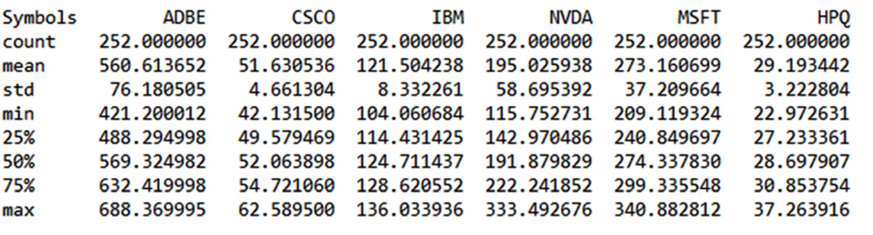
Figure 9.7 – The statistics of the portfolios

Analyzing the previous table, note that there are 252 records. These are the days when the stock exchange was opened in 2021. Let’s take note of it, as this data will be useful later on. We also note that the values in the columns have very different ranges due to the different values of the stocks. To better understand the trend of stocks, it is better to draw graphs. Let’s do this next:

fig, axs = plt.subplots(3, 2, figsize=(20,10))
axs[0, 0].plot(StockClose['ADBE'])
axs[0, 0].set_title('ADBE')
axs[0, 1].plot(StockClose['CSCO'])
axs[0, 1].set_title('CSCO')
axs[1, 0].plot(StockClose['IBM'])
axs[1, 0].set_title('IBM')
axs[1, 1].plot(StockClose['NVDA'])
axs[1, 1].set_title('NVDA')
axs[2, 0].plot(StockClose['MSFT'])
axs[2, 0].set_title('MSFT')
axs[2, 1].plot(StockClose['HPQ'])
axs[2, 1].set_title('HPQ')

In order to make an easy comparison between the trends of the six stocks, we have traced six subplots that are ordered in three rows and two columns. We used the subplots() function of the matplotlib library. This function returns a tuple containing a figure object and axes. So, when you use fig and axs = plt.subplots(), you unpack this tuple into the variables of fig and axs. Having fig is useful if you want to change the attributes at the figure level or save the figure as an image file later. The variable, axs, allows us to set the attributes of the axes of each subplot. In fact, we called this variable to define what to draw in each subplot by calling it with the row-column indices of the chart matrix. In addition, for each chart, we also printed the title that allows us to understand which ticker it refers to.

The following plots are shown:

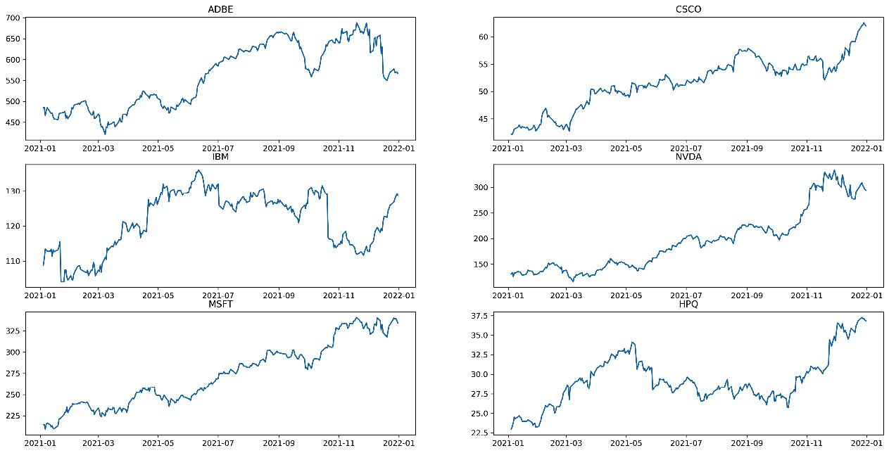
Figure 9.8 – The graphs of the statistics

4. After taking a quick look at the trend of stocks, the time has come to evaluate the returns:

   StockReturns = StockClose.pct_change()

   print(StockReturns.tail())

The pct.change() function returns the percentage change between the current close price and the previous value. By default, the function calculates the percentage change from the immediately preceding row.

The concept of the percentage variation of a time series is linked to the concept of the return of a stock price. The returns-based approach provides for the normalization of data, which is an operation of fundamental importance to evaluate the relationships between variables characterized by different metrics. These concepts have been explored in this chapter’s Using Monte Carlo methods for stock price prediction section. Note that we have only referred to some of them.

We then printed the queue of the returned DataFrame to analyze its contents. The following results are returned:

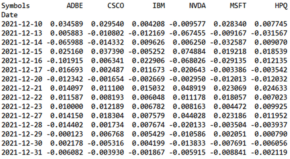
Figure 9.9 – The stock returns DataFrame

In the previous table, the minus sign indicates a negative return with a loss, at least daily.

5. Now, we are ready to assess the investment risk of a substantial portfolio of stocks of these prestigious companies. To do this, we need to set some variables and calculate others:

   PortfolioValue = 1000000000.00

   ConfidenceValue = 0.95

   Mu = np.mean(StockReturns)

   Sigma = np.std(StockReturns)

To start, we set the value of our portfolio; it is a billion dollars. These figures should not frighten you. For a bank that manages numerous investors, achieving this investment value is not difficult. So, we set the confidence interval. Previously, we said that VaR is based on this value. Subsequently, we started to calculate some fundamental quantities for the VaR calculation. I am referring to the mean and standard deviation of returns. To do this, we used the related numpy functions: np.mean() and np.std.

We continue to set the parameters necessary for calculating VaR:

WorkingDays2021 = 252.
AnnualizedMeanStockRet = MeanStockRet/WorkingDays2021
AnnualizedStdStockRet = 
                StdStockRet/np.sqrt(WorkingDays2021)

Previously, we saw that the data extracted from the finance section of the Yahoo website contained 252 records. This is the number of working days of the stock exchange in 2021, so we set this value. So, let’s move on to annualizing the mean and the standard deviation just calculated. This is because we want to calculate the annual risk index of the stocks. For the annualization of the average, it is enough to divide by the number of working days, while for the standard deviation, we must divide by the square root of the number of working days.

6. Now, we have all the data we need to calculate VaR:

   INPD = norm.ppf(1-ConfidenceValue,AnnualizedMeanStockRet,

                      AnnualizedStdStockRet)

   VaR = PortfolioValue*INPD

To start, we calculate the inverse normal probability distribution with a risk level of 1 confidence, mean, and standard deviation. This technique involves the construction of a probability distribution, starting from the three parameters we have mentioned. In this case, we work backward, starting from some distribution statistics, and try to reconstruct the starting distribution. To do this, we used the norm.ppf() function of the SciPy library.

The norm() function returns a normal continuous random variable. The acronym, ppf, stands for percentage point function, which is another name for the quantile function. The quantile function, associated with a probability distribution of a random variable, specifies the value of the random variable so that the probability that the variable is less than or equal to that value is equal to the given probability.

At this point, VaR is calculated by multiplying the inverse normal probability distribution obtained by the value of the portfolio. To make the value obtained more readable, it was rounded to the first two decimal places:

RoundVaR=np.round_(VaR,2)

Finally, the results obtained were printed, one for each row, to make the comparison simple:

for i in range(len(StockList)):
    print("Value-at-Risk for", StockList[i], 
                   "is equal to ",RoundVaR[i])

The following results are returned:

Value-at-Risk for ADBE is equal to  -1901394.1
Value-at-Risk for CSCO is equal to  -1244064.53
Value-at-Risk for IBM is equal to  -1485931.31
Value-at-Risk for NVDA is equal to  -2922034.18
Value-at-Risk for MSFT is equal to  -1358218.7
Value-at-Risk for HPQ is equal to  -2020466.29

The stocks that returned the highest risk were NVDA and HPQ, while the one that returned the lowest risk was the CSCO stock.

Summary

In this chapter, we applied the concepts of simulation based on Monte Carlo methods and, more generally, on the generation of random numbers to real cases related to the world of financial engineering. We started by defining the model based on Brownian motion, which describes the uninterrupted and irregular movement of small particles when immersed in a fluid. We learned how to describe the mathematical model, and then we derived a practical application that simulates a random walk as a Wiener process.

Afterward, we dealt with another practical case of considerable interest – that is, how to use Monte Carlo methods to predict the stock prices of the famous company Amazon. We started to explore the trend of Amazon shares in the last 10 years, and we performed simple statistics to extract preliminary information on any trends that we confirmed through visual analysis. Subsequently, we learned to treat the trend of stock prices as a time series, calculating the daily return. We then addressed the problem with the BS model, defining the concepts of drift and standard Brownian motion. Finally, we applied the Monte Carlo method to predict possible scenarios relating to the trend of stock prices.

As a final practical application, we assessed the risk associated with a portfolio of shares of some of the most famous technology companies listed on the NASDAQ market. We first defined the concept of referrals connected to a financial asset, and then we introduced the concept of VaR. Subsequently, we implemented an algorithm that, given a confidence interval and a time horizon, calculates VaR based on the daily returns returned by the historical data of the stock prices.

In the next chapter, we will learn about the basic concepts of artificial neural networks, how to apply feedforward neural network methods to our data, and how the neural network algorithm works. Then, we will take a look at the basic concepts of a deep neural network and how to use neural networks to simulate a physical phenomenon.