10

Simulating Physical Phenomena Using Neural Networks

Neural networks are exceptionally effective at getting good characteristics for highly structured data. Physical phenomena are conditioned by numerous variables that can be easily measured through modern sensors. In this way, big data is produced that is difficult to deal with using classic techniques. Neural networks lend themselves to simulating complex environments.

In this chapter, we will learn how to develop models based on artificial neural networks (ANNs) to simulate physical phenomena. We will start by exploring the basic concepts of neural networks, and then we will examine their architecture and main elements. We will demonstrate how to train a network to update its weights. Then, we will apply these concepts to a practical use case to solve a regression problem. In the last part of the chapter, we will analyze deep neural networks.

In this chapter, we’re going to cover the following topics:

• Introducing the basics of neural networks
• Understanding feedforward neural networks
• Simulating airfoil self-noise using ANNs
• Approaching deep neural networks
• Exploring graph neural networks (GNNs)
• Simulation modeling using neural network techniques

Technical requirements

In this chapter, we will learn how to use ANNs to simulate complex environments. To understand the topics, a basic knowledge of algebra and mathematical modeling is needed.

To work with the Python code in this chapter, you need the following files (available on GitHub at https://github.com/PacktPublishing/Hands-On-Simulation-Modeling-with-Python-Second-Edition):

• airfoil_self_noise.py
• concrete_quality.py

Introducing the basics of neural networks

ANNs are numerical models developed with the aim of reproducing simple neural activities of the human brain, such as object identification and voice recognition. The structure of an ANN is composed of nodes that, similar to the neurons present in a human brain, are interconnected with each other through weighted connections, which reproduce the synapses between neurons.

The system output is updated until it iteratively converges via the connection weights. The information deriving from experimental activities is used as input data and the result processed by the network is returned as an output. The input nodes represent the predictive variables, and the output neurons are represented by the dependent variables. We use the predictive variables to process the dependent variables.

ANNs are very versatile in simulating regression and classification problems. They can learn the process of working out the solution to a problem by analyzing a series of examples. In this way, the researcher is released from the difficult task of building a mathematical model of the physical system, which, in some cases, is impossible to represent.

Understanding biological neural networks

ANNs are based on a model that draws inspiration from the functioning principles of the human brain and how the human brain processes the information that comes to it from the peripheral organs. In fact, ANNs consist of a series of neurons that can be thought of as individual processors, since their basic task is to process the information that is provided to them at the input. This processing is similar to the functioning of a biological neuron, which receives electrical signals, processes them, and then transmits the results to the next neuron. The essential elements of a biological neuron include the following:

• Dendrites
• Synapses
• Body cells
• Axon

The information is processed by the biological neuron according to the following steps:

1. Dendrites get information from other neurons in the form of electrical signals.
2. The flow of information occurs through the synapses.
3. The dendrites transmit this information to the cell body.
4. In the cell body, the information is added together.
5. If the result exceeds a threshold limit, the cell reacts by passing the signal to another cell. The passage of information takes place through the axon.

The following diagram shows the essential elements of the structure of a biological neuron:

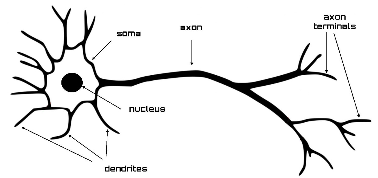
Figure 10.1: The structure of a neuron

Synapses assume the role of neurotransmitters; in fact, they can exert an excitatory or inhibitory action against the neuron that is immediately after it. This effect is regulated by the synapses through the weight that is associated with them. In this way, each neuron can perform a weighted sum of the inputs, and if this sum exceeds a certain threshold, it activates the next neuron.

Important note

The processing performed by the neuron lasts for a few milliseconds. From a computational point of view, it represents a relatively long time. So, we could say that this processing system, taken individually, is relatively slow. However, as we know, it is a model based on quantity; it is made up of a very high number of neurons and synapses that work simultaneously and in parallel.

In this way, the processing operations that are performed are very effective, and they allow us to obtain results in a relatively short period of time. We can say that the strength of neural networks lies in the teamwork of neurons. Taken individually, they do not represent a particularly effective processing system; however, taken together, they represent an extremely high-performing simulation model.

The functioning of a brain is regulated by neurons and represents an optimized machine that can solve even complex problems. It is a simple structure, improved over time through the evolution of the species. It has no central control; the areas of the brain are all active in carrying out a task, which is aimed at solving a problem. The workings of all parts of the brain take place in a contributory way, and each part contributes to the result. In addition to this, the human brain is equipped with a very effective error regulation system. In fact, if a part of the brain stops working, the operations of the entire system continue to be performed, even if with a lower performance.

Exploring ANNs

As we have anticipated, a model based on ANNs draws inspiration from the functioning of the human brain. In fact, an artificial neuron is similar to a biological neuron in that it receives information as input derived from another neuron. A neuron’s input represents the output of the neuron that is found immediately before in the architecture of a model based on neural networks.

Each input signal to the neuron is then multiplied by the corresponding weight. It is then added to the results obtained by the other neurons to process the activation level of the next neuron. The essential elements of the architecture of a model based on ANNs include the neurons that are distinguished from the input neurons and the output neurons by the number of layers of synapses and by the connections between these neurons. The following diagram shows the typical architecture of an ANN:

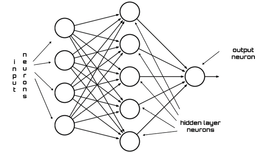
Figure 10.2: Architecture of an ANN

The input signals, which represent the information detected by the environment, are sent to the input layer of the ANN. In this way, they travel, in parallel, along with the connections through the internal nodes of the system and up to the output. The architecture of the network, therefore, returns a response from the system. Put simply, in a neural network, each node is able to process only local information with no knowledge of the final goal of the processing and not keeping any memory of the latter. The result obtained depends on the architecture of the network and the values assumed by the artificial synapses.

There are cases in which a single synapse layer is unable to return an adequate network response to the signal supplied at the input. In these cases, multiple layers of synapses are required because a single layer is not enough. These networks are called deep neural networks. The network response is obtained by treating the activation of one layer of neurons at a time and then proceeding from the input to the output, passing through the intermediate layers.

Important note

The ANN target is the result of the calculation of the outputs performed for all the neurons, so an ANN is presented as a set of mathematical function approximations.

The following elements are essential in an ANN architecture:

• Weights
• Bias
• Layers
• Activation functions

In the following sections, we will deepen our understanding of these concepts.

Describing the structure of the layers

In the architecture of an ANN, it is possible to identify the nodes representing the neurons distributed in a form that provides a succession of layers. In a simple structure of an ANN, it is possible to identify an input layer, an intermediate layer (hidden layer), and an output layer, as shown in the following diagram:

Figure 10.3: The various layers of an ANN

Each layer has its own task, which it performs through the actions of the neurons it contains. The input layer is intended to introduce the initial data into the system for further processing by the subsequent layers. From the input level, the workflow of the ANN begins.

Important note

In the input layer, artificial neurons have a different role to play in some passive way because they do not receive information from the previous levels. In general, they receive a series of inputs and introduce information into the system for the first time. This level then sends the data to the next levels where the neurons receive weighted inputs.

The hidden layer in an ANN is interposed between input levels and output levels. The neurons of the hidden layer receive a set of weighted inputs and produce an output according to the indications received from an activation function. It represents the essential part of the entire network since it is here that the magic of transforming the input data into output responses takes place.

Hidden levels can operate in many ways. In some cases, the inputs are weighted randomly, while in others they are calibrated through an iterative process. In general, the neuron of the hidden layer functions as a biological neuron in the brain. That is, it takes its probabilistic input signals, processes them, and converts them into an output corresponding to the axon of the biological neuron.

Finally, the output layer produces certain outputs for the model. Although they are very similar to other artificial neurons in the neural network, the type and number of neurons in the output layer depend on the type of response the system must provide. For example, if we are designing a neural network for the classification of an object, the output layer will consist of a single node that will provide us with this value. In fact, the output of this node must simply provide a positive or negative indication of the presence or absence of the target in the input data. For example, if our network must perform an object classification task, then this layer will contain only one neuron destined to return this value. This is because this neuron must return a binary signal, that is, a positive or negative response that signals the presence or absence of the object among the data provided as input.

Analyzing weights and biases

In a neural network, weights represent a crucial factor in converting an input signal into the system response. They represent a factor such as the slope of a linear regression line. In fact, the weight is multiplied by the inputs and the result is added to the other contributions. These are numerical parameters that determine the contribution of a single neuron in the formation of the output.

If the inputs are x1, x2, … xn, and the synaptic weights to be applied to them are denoted as w1, w2, … wn, the output returned by the neuron is expressed through the following formula:

The previous formula is a matrix multiplication to reach the weighted sum. The neuron elaboration can be denoted as follows:

In the previous formula, the bias assumes the role of the intercept in a linear equation. The bias represents an additional parameter that is used to regulate the output along with the weighted sum of the inputs to the neuron.

The input of the next layer is the output of the neurons in the previous layer, as shown in the following diagram:

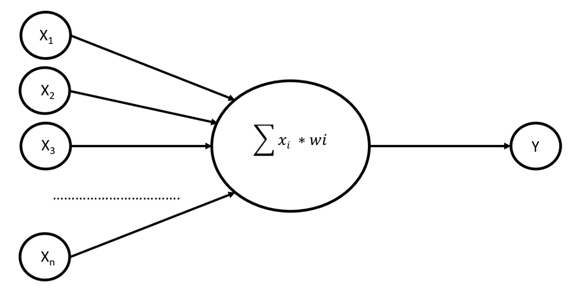
Figure 10.4: Output of the neurons

The schema presented in the previous diagram explains the role played by the weight in the formation of a neuron. Note that the input provided to the neuron is weighed with a real number that reproduces the activity of the synapse of a biological neuron. When the weight value is positive, the signal has an excitatory activity. If, on the other hand, the value is negative, the signal is inhibitory. The absolute value of the weight indicates the strength of the contribution to the formation of the system response.

Explaining the role of activation functions

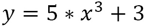
The abstraction of neural network processing is primarily obtained via the activation functions. This is a mathematical function that transforms the input into output and controls a neural network process. Without the contribution of activation functions, a neural network can be assimilated into a linear function. A linear function occurs when the output is directly proportional to the input. For example, let’s analyze the following equation:

In the previous equation, the exponent of x is equal to 1. This is the condition for the function to be linear: it must be a first-degree polynomial. It is a straight line with no curves. Unfortunately, most real-life problems are nonlinear and complex in nature. To treat nonlinearity, activation functions are introduced in neural networks. Recall that, for a function to be nonlinear, it is sufficient that it is a polynomial function of a degree higher than the first. For example, the following equation defines a nonlinear function of the third degree:

The graph of a nonlinear function is curved and adds to the complexity factor. Activation functions give the nonlinearity property to neural networks and make them true universal function approximators.

There are many activation functions available for a neural network to use. The most used activation functions are listed here:

• Sigmoid: The sigmoid function is a mathematical function that produces a sigmoidal curve, which is a characteristic curve for its S shape. This is one of the earliest and most used activation functions. This squashes the input to any value between 0 and 1 and makes the model logistic in nature.
• Unit step: A unit step activation function is a much-used feature in neural networks. The output assumes a value of 0 for a negative argument and a value of 1 for a positive argument. The range is between 0 and 1 and the output is binary in nature. These types of activation functions are useful for binary schemes.
• Hyperbolic tangent: This is a nonlinear function, defined in the range of values -1 to 1, so you do not need to worry about activations blowing up. One thing to clarify is that the gradient is stronger for tanh than sigmoid. Deciding between sigmoid and tanh will depend on your gradient strength requirement. Like sigmoid, tanh also has the missing slope problem.
• Rectified Linear Unit (ReLU): This is a function with linear characteristics for parts of the existing domain that will output the input directly if it is positive; otherwise, it will output 0. The range of output is between 0 and infinity. ReLU finds applications in computer vision and speech recognition using deep neural networks.

The previously listed activation functions are shown in the following diagram:

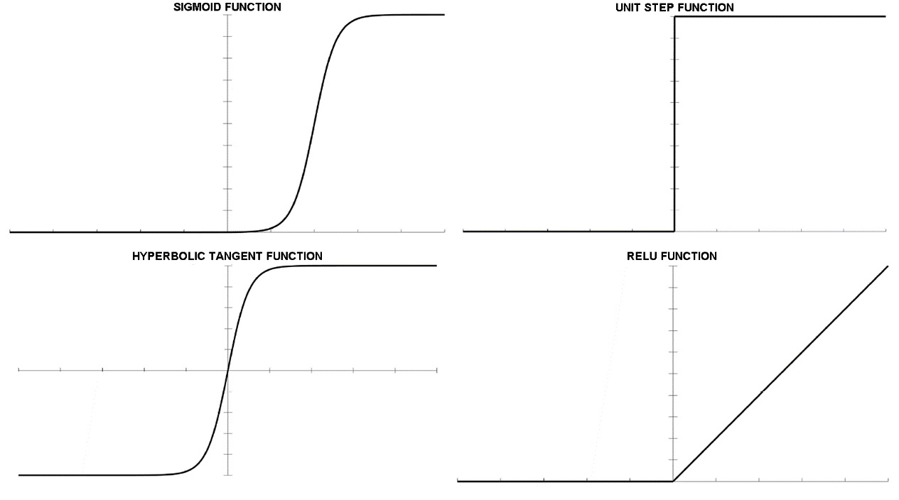
Figure 10.5: Representation of activation functions

Now we will look at the simple architecture of a neural network, which shows us how the flow of information proceeds.

Let’s see how a feedforward neural network is structured.

Understanding feedforward neural networks

The processing from the input layer to the hidden layer(s) and then to the output layer is called feedforward propagation. The transfer function is applied at each hidden layer, and then the activation function value is propagated to the next layer. The next layer can be another hidden layer or the output layer.

Important note

The term “feedforward” is used to indicate the networks in which each node receives connections only from the lower layers. These networks emit a response for each input pattern but fail to capture the possible temporal structure of the input information or exhibit endogenous temporal dynamics.

Exploring neural network training

The learning ability of an ANN is manifested in the training procedure. This represents the crucial phase of the whole algorithm as it is through the characteristics extracted during training that the network acquires the ability to generalize. The training takes place through a comparison between a series of inputs corresponding to known outputs and those supplied by the model. At least, this is what happens in the case of supervised algorithms in which the labeled data is compared with that provided by the model.

The results achieved by the model are influenced by the data used in the training phase—to obtain good performance, the data used must be sufficiently representative of the phenomenon. From this, we can understand the importance of the dataset used in this phase, which is called the training set.

To understand the procedure through which a neural network learns from data, let’s consider a simple example. We will analyze the training of a neural network with a single hidden level. Let’s say that the input level has a neuron, and the network will have to face a binary classification problem—only two output values of either 0 or 1.

The training of the network will take place according to the following steps:

1. Enter the input in the form of a data matrix.
2. Initialize the weights and biases with random values. This step will be performed once, at the beginning of the procedure only. Later, the weights and biases will be updated through the error propagation process.
3. Repeat steps 4 to 9 until the error is minimized.
4. Apply inputs to the network.
5. Calculate the output for each neuron from the input level to the hidden levels to the output level.
6. Calculate the error on the outputs: less real than expected.
7. Use the output error to calculate the error signals for the previous layers. The partial derivative of the activation function is used to calculate the error signals.
8. Use the error signals to calculate the weight adjustments.
9. Apply the weight adjustments.

Steps 4 and 5 represent the direct propagation phase, while steps 6 to 9 represent the backpropagation phase.

The most used method to train a network through the adjustment of neuron weights is the delta rule, which compares the network output with the desired values. Subtract the two values and the difference is used to update all of the input weights, which have different values of zero. The process is repeated until convergence is achieved.

The following diagram shows the weight adjustment procedure:

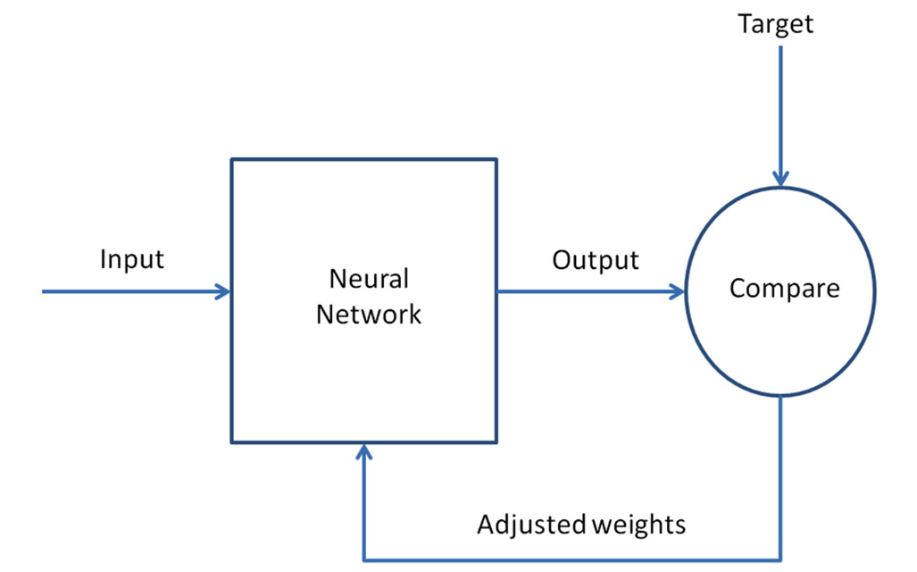
Figure 10.6: The weight adjustment procedure

The training procedure is extremely simple: it is a simple comparison between the calculated values and the labeled values. The difference between the weighted input values and the expected output values is calculated from the comparison—the difference, which represents the evaluation error between the calculated and expected values, is used to recalculate all of the input weights. It is an iterative procedure that is repeated until the error between the expected and calculated value approaches zero.

The training phase can be performed with the backpropagation technique in combination with an optimization method such as stochastic gradient descent. Backpropagation is one of the most widely used algorithms to train neural networks, both single-layer and multi-layer. This algorithm aims to modify the weights of the neurons in the network to minimize the error given by the difference between the output vector obtained and the desired one. Numerical optimization is iterative and requires the calculation of the gradient of the cost function with respect to weights and biases. For each iteration of the algorithm, the gradient calculation requires several operations equal to the number of coefficients. The backpropagation algorithm requires the calculation of the gradient only in the last layer, which is then propagated backward to obtain the gradient in the previous layers. The stochastic descent of the gradient, as seen in detail in Chapter 7, Using Simulation to Improve and Optimize Systems, aims to reach the lowest point of the cost function. In more technical terms, the gradient represents a derivative indicating the slope or slope of the objective function.

After having analyzed in detail the architecture of the ANNs, we will now see a practical case of elaboration of an ANN-based model to solve a physical problem.

Simulating airfoil self-noise using ANNs

The noise generated by an airfoil is due to the interaction between a turbulent airflow and the aircraft’s airfoil blades. Predicting the acoustic field in these situations requires an aeroacoustics methodology that can operate in complex environments. Additionally, the method that is used must avoid the formulation of coarse hypotheses regarding geometry, compactness, and content of the frequency of sound sources. The prediction of the sound generated by a turbulent flow must, therefore, correctly model both the physical phenomena of sound propagation and the turbulence of the flow. Since these two phenomena manifest energy and scales of very different lengths, the correct prediction of the sound generated by a turbulent flow is not easy to model.

Aircraft noise is a crucial topic for the aerospace industry. The NASA Langley Research Center has funded several strands of research to effectively study the various mechanisms of a self-noise airfoil. Interest was motivated by its importance for broadband helicopter rotors, wind turbines, and cell noises. The goal of these studies, then, focused on the challenge of reducing external noises generated by the entire cell of an aircraft by 10 decibels.

In this example, we will elaborate on a model based on ANNs to predict self-noise airfoils from a series of airfoil data measured in a wind tunnel.

Important note

The dataset we will use was developed by NASA in 1989 and is available on the UCI Machine Learning Repository site. The UCI Machine Learning Repository is available at https://archive.ics.uci.edu/ml/datasets/Airfoil+Self-Noise.

The dataset was built using the results of a series of aerodynamic and acoustic tests on sections of aerodynamic blades performed in an anechoic wind tunnel.

The following list shows the features of the dataset:

• Number of instances: 1,503
• Number of attributes: 6
• Dataset characteristics: multivariate
• Attribute characteristics: real
• Dataset date: 2014-03-04

The following list presents a brief description of the attributes:

• Frequency: Frequency in Hertz (Hz)
• AngleAttack: angle of attack in degrees
• ChordLength: chord length in meters
• FSVelox: free-stream velocity in meters per second
• SSDT: suction-side displacement thickness (SSDT) in meters
• SSP: scaled sound pressure level in decibels

In the six attributes we have listed, the first five represent the predictors, and the last one represents the response of the system that we want to simulate. It is, therefore, a regression problem because the answer has continuous values. In fact, it represents the self-noise airfoil, in decibels, measured in the wind tunnel.

Importing data using pandas

The first operation we will perform is the importing of data, which, as we have already mentioned, is available on the UCI website. As always, we will analyze the code line by line:

1. We start by importing the libraries. In this case, we will operate differently from what has been done so far. We will not import all of the necessary libraries at the beginning of the code, but we will introduce them in correspondence with their use and we will illustrate their purposes in detail:

   import pandas as pd

The pandas library is an open source, BSD-licensed library that provides high-performance, easy-to-use data structures, and data analysis tools for the Python programming language. It offers data structures and operations for manipulating numerical data in a simple way. We will use this library to import the data contained in the dataset retrieved from the UCI website.

The UCI dataset does not contain a header, so it is necessary to insert the names of the variables in another variable. Now, let’s put these variable names in the following list:

ASNNames= ['Frequency','AngleAttack','ChordLength','FSVelox','SSDT','SSP']

2. Now we can import the dataset. This is available in .dat format, and, to make your job easier, it has already been downloaded and is available in this book’s GitHub repository:

   ASNData = pd.read_csv('airfoil_self_noise.dat', delim_whitespace=True, names=ASNNames)

To import the .dat dataset, we used the read_csv module of the pandas library. In this function, we passed the filename and two other attributes, namely delim_whitespace and names. The first specifies whether or not whitespace will be used as sep, and the second specifies a list of column names to use.

Important note

Remember to set the path so that Python can find the .dat file to open.

Before beginning with data analysis through ANN regression, we perform an exploratory analysis to identify how data is distributed and extract preliminary knowledge. To display the first 20 rows of the imported DataFrame, we can use the head() function, as follows:

print(ASNData.head(20))

The pandas head() function gets the first n rows of a pandas DataFrame. In this case, it returns the first 20 rows for the ASNData object based on position. It is used for quickly testing whether our dataset has the right type of data in it. This function, with no arguments, gets the first five rows of data from the DataFrame.

The following data is printed:

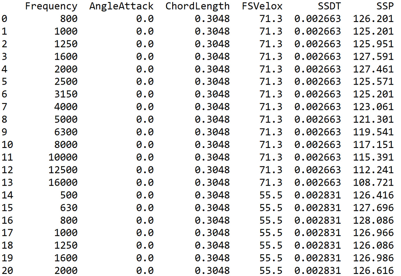
Figure 10.7: DataFrame output

To extract further information, we can use the info() function, as follows:

print(ASNData.info())

The info() method returns a concise summary of the ASNData DataFrame, including the dtypes index and dtypes column, non-null values, and memory usage.

The following results are returned:

<class 'pandas.core.frame.DataFrame'>
RangeIndex: 1503 entries, 0 to 1502
Data columns (total 6 columns):
Frequency      1503 non-null int64
AngleAttack    1503 non-null float64
ChordLength    1503 non-null float64
FSVelox        1503 non-null float64
SSDT           1503 non-null float64
SSP            1503 non-null float64
dtypes: float64(5), int64(1)
memory usage: 70.5 KB
None

By reading the information returned by the info method, we can confirm that it is 1,503 instances and six variables. In addition to this, the types of variables returned to us are five float64 variables and one int64 variable.

3. To obtain a first screening of the data contained in the ASNData DataFrame, we can compute a series of basic statistics. We can use the describe() function in the following way:

   BasicStats = ASNData.describe()

   BasicStats = BasicStats.transpose()

   print(BasicStats)

The describe() function produces descriptive statistics that return the central tendency, dispersion, and shape of a dataset’s distribution, excluding Not-a-Number (NaN) values. It is used for both numeric and object series, as well as the DataFrame column sets of mixed data types. The output will vary depending on what is provided. In addition to this, we have transposed the statistics to appear better on the screen and to make it easier to read the data.

The following statistics are printed:

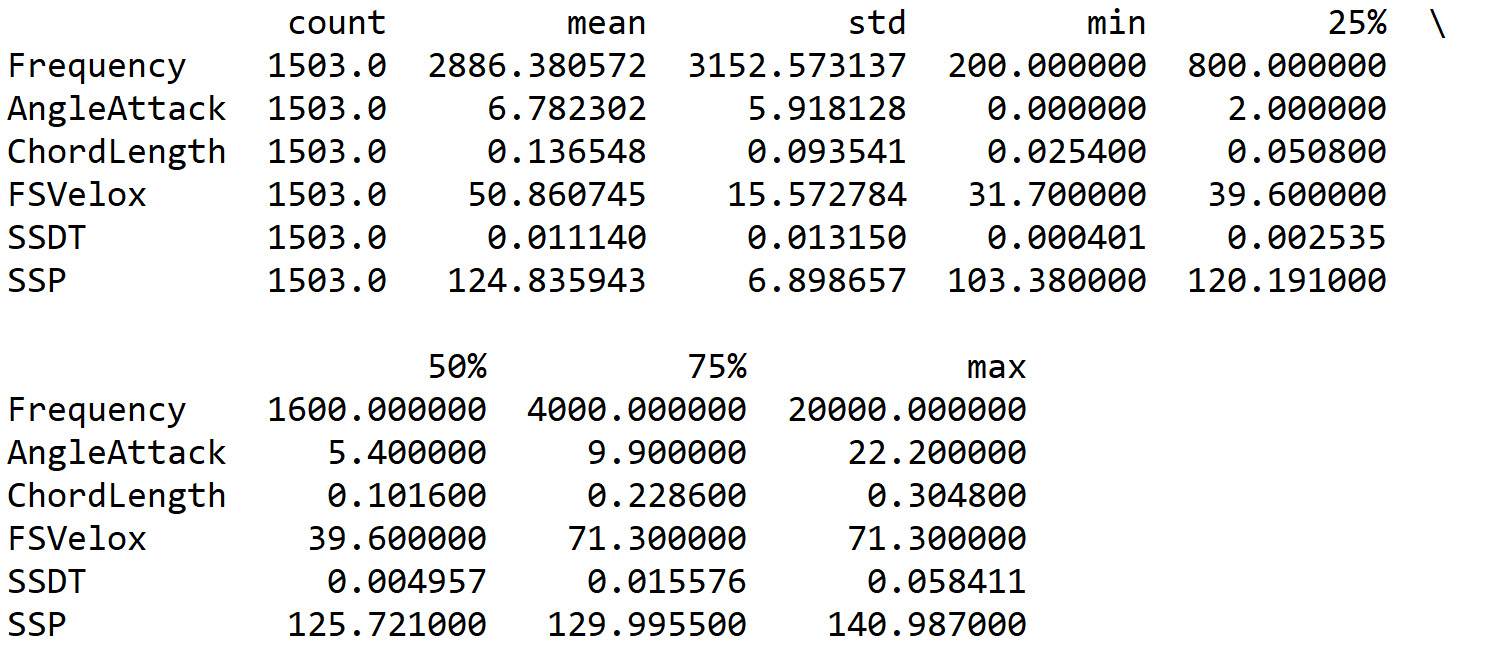
Figure 10.8: Basic statistics from the DataFrame

From the analysis of the previous table, we can extract useful information. First of all, we can note that the data shows great variability. The average of the values ranges from approximately 0.14 to 2,886. Not only that, but some variables have a very large standard deviation. For each variable, we can easily recover the minimum and maximum. In this way, we can note that the interval of the analyzed frequencies goes from 200 to 20,000 Hz. These are just some considerations; we can recover many others.

Scaling the data using sklearn

In the statistics extracted using the describe() function, we have seen that the predictor variables (frequency, angle of attack, chord length, free-stream velocity, and SSDT) have an important variability. In the case of predictors with different and varied ranges, the influence on the system response by variables with a larger numerical range could be greater than those with a lower numeric range. This different impact could affect the accuracy of the prediction. Actually, we want to do exactly the opposite, that is, improve predictive accuracy and reduce the sensitivity of the model from features that can affect prediction due to a wide range of numerical values.

To avoid this phenomenon, we can reduce the values so that they fall within a common range, guaranteeing the same characteristics of variability possessed by the initial dataset. In this way, we will be able to compare variables belonging to different distributions and variables expressed in different units of measurement.

Important note

Recall how we rescale the data before training a regression algorithm. This is a good practice. Using a rescaling technique, data units are removed, allowing us to compare data from different locations easily.

We then proceed with data rescaling. In this example, we will use the min-max method (usually called feature scaling) to get all of the scaled data in the range 0–1. The formula to achieve this is as follows:

To do feature scaling, we can apply a preprocessing package offered by the sklearn library. This library is a free software machine learning library for the Python programming language. The sklearn library offers support for various machine learning techniques, such as classification, regression, and clustering algorithms, including support vector machines (SVMs), random forests, gradient boosting, k-means, and DBSCAN. sklearn is created to work with various Python numerical and scientific libraries, such as NumPy and SciPy:

Important note

To import a library that is not part of the initial distribution of Python, you can use the pip install command, followed by the name of the library. This command should be used only once and not every time you run the code.

1. The sklearn.preprocessing package contains numerous common utility functions and transformer classes to transform the features in a way that works with our requirements. Let’s start by importing the package:

   from sklearn.preprocessing import MinMaxScaler

To scale features between the minimum and maximum values, the MinMaxScaler function can be used. In this example, we want to rescale the data between zero and one so that the maximum absolute value of each feature is scaled to unit size.

2. Let’s start by setting the scaler object:

   ScalerObject = MinMaxScaler()
3. To get validation of what we are doing, we will print the object just created in order to check the set parameters:

   print(ScalerObject.fit(ASNData))

The following result is returned:

MinMaxScaler(copy=True, feature_range=(0, 1))

4. Now, we can apply the MinMaxScaler() function, as follows:

   ASNDataScaled = ScalerObject.fit_transform(ASNData)

The fit_transform() method fits to the data and then transforms it. Before applying the method, the minimum and maximum values that are to be used for later scaling are calculated. This method returns a NumPy array object.

5. Recall that the initial data had been exported in the pandas DataFrame format. Scaled data should also be transformed into the same format in mdoo to be able to apply the functions available for pandas DataFrames. The transformation procedure is easy to perform; just apply the pandas DataFrame() function as follows:

   ASNDataScaled = pd.DataFrame(ASNDataScaled, columns=ASNNames)
6. At this point, we can verify the results obtained with data scaling. Let’s compute the statistics using the describe() function once again:

   summary = ASNDataScaled.describe()

   summary = summary.transpose()

   print(summary)

The following statistics are printed:

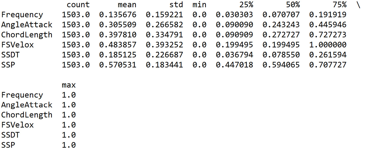
Figure 10.9: Output with scaled data

From the analysis of the previous table, the result of the data scaling appears evident. Now all six variables have values between 0 and 1.

Viewing the data using Matplotlib

Now, we will try to have a confirmation of the distribution of the data through a visual approach:

1. To start, we will draw a boxplot, as follows:

   import matplotlib.pyplot as plt

   boxplot = ASNDataScaled.boxplot(column=ASNNames)

   plt.show()

A boxplot, also referred to as a whisker chart, is a graphical description used to illustrate the distribution of data using dispersion and position indices. The rectangle (box) is delimited by the first quartile (25th percentile) and the third quartile (75th percentile) and divided by the median (50th percentile). In addition, there are two whiskers, one upper and one lower, indicating the maximum and minimum distribution values, excluding any anomalous values.

Matplotlib is a Python library for printing high-quality graphics. With matplotlib, it is possible to generate graphs, histograms, bar graphs, power spectra, error graphs, scatter graphs, and more with just a few commands. This is a collection of command-line functions such as those provided by the MATLAB software.

As we mentioned earlier, the scaled data is in pandas DataFrame format. So, it is advisable that you use the pandas.DataFrame.boxplot function. This function makes a boxplot from the DataFrame columns, which are optionally grouped by some other columns.

The following diagram is printed:

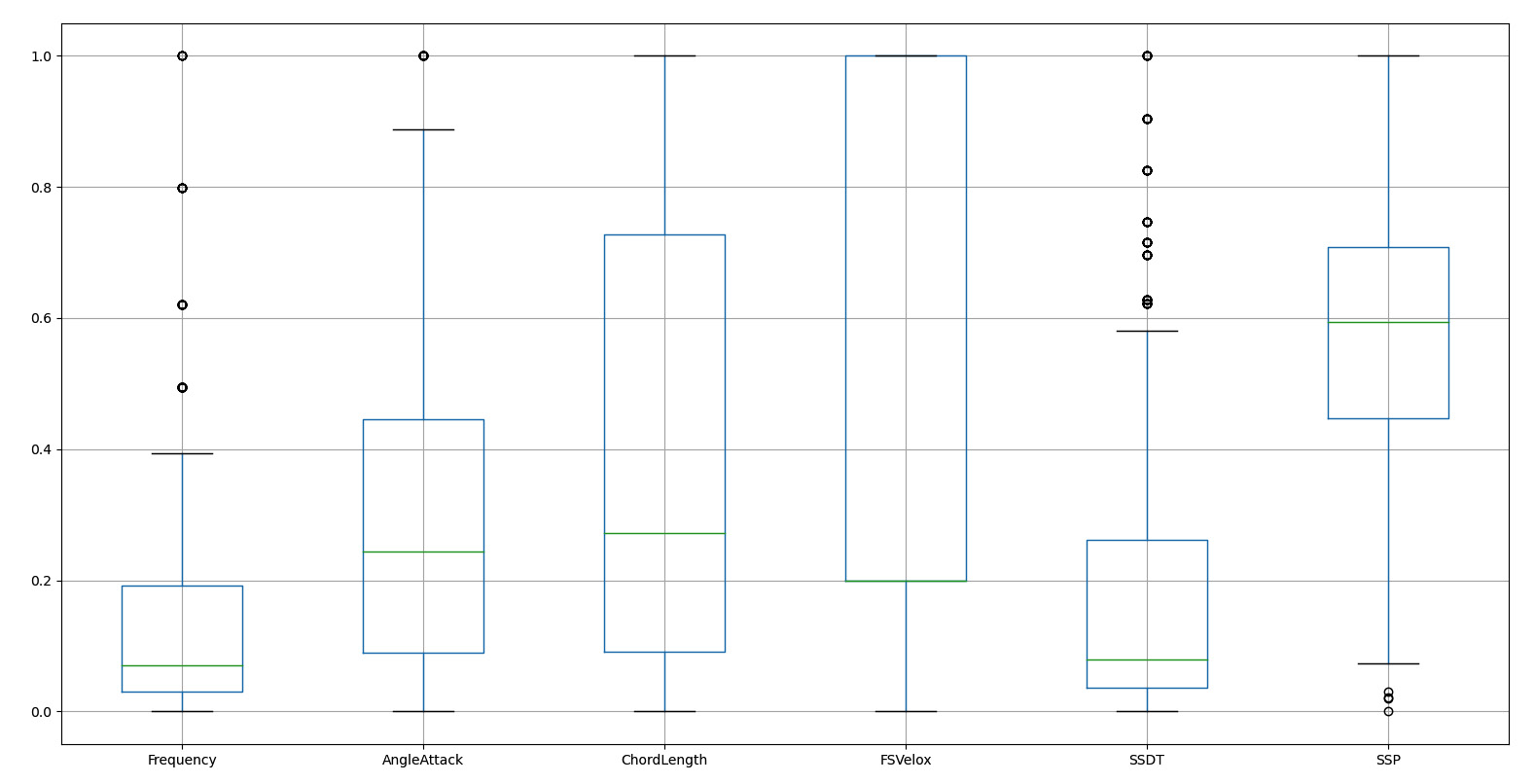
Figure 10.10: Boxplot of the DataFrame

In the previous diagram, you can see that there are some anomalous values indicated by small circles at the bottom and side of the extreme mustache of each box. Three variables have these values, called outliers, and their presence can create problems in the construction of the model. Furthermore, we can verify that all the variables are contained in the extreme values that are equal to 0 and 1; this is the result of data scaling. Finally, some variables such as FSVelox show a great variability of values compared to others, for example, SSDT.

We will now measure the correlation between the predictors and the response variable. A technique for measuring the relationship between two variables is offered by correlation, which can be obtained using covariance. To calculate the correlation coefficients in Python, we can use the pandas.DataFrame.corr() function. This function computes the pairwise correlation of columns, excluding NA/null values. Three procedures are offered, as follows:

• pearson (standard correlation coefficient)
• kendall (Kendall Tau correlation coefficient)
• spearman (Spearman rank correlation)

Important note

Remember that the correlation coefficient of two random variables is a measure of their linear dependence.

2. Let’s calculate the correlation coefficients for the data scaled:

   CorASNData = ASNDataScaled.corr(method='pearson')

   with pd.option_context('display.max_rows', None,  

       'display.max_columns', CorASNData.shape[1]):

   print(CorASNData)

To show all data columns on a screenshot, we used the option_context function. The following results are returned:

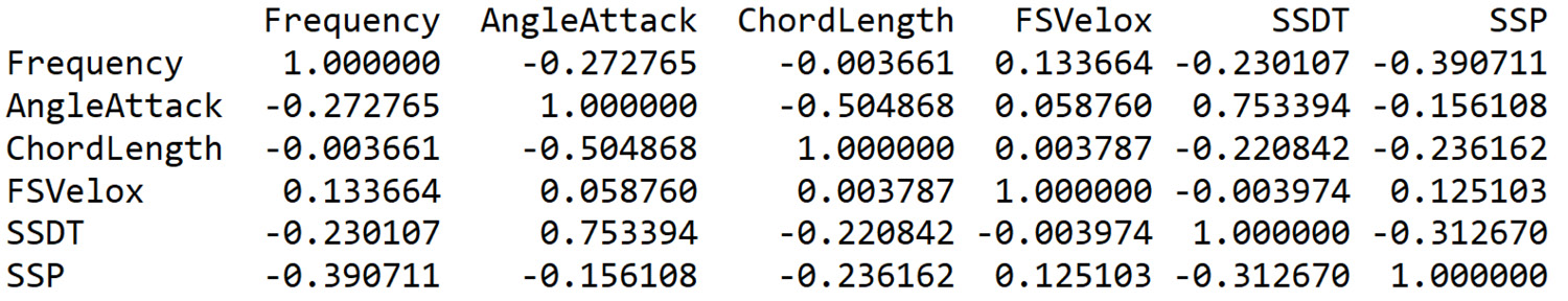
Figure 10.11: Data columns in the DataFrame

We are interested in studying the possible correlation between the predictors and the system response. So, to do this, it will be sufficient to analyze the last row of the previous table. Recall that the values of the various correlation indices vary between -1 and +1; both extreme values represent perfect relationships between the variables, while 0 represents the absence of a relationship. This is if we consider linear relationships. Based on this, we can say that the predictors that show a greater correlation with the response SSP are Frequency and SSDT. Both show a negative correlation.

To see visual evidence of the correlation between the variables, we can plot a correlogram. A correlogram graphically presents a correlation matrix. It is used to focus on the most correlated variables in a data table. In a correlogram, correlation coefficients are shown in a nuance that depends on our values. Next to the graph, a colored bar will be proposed in which the corresponding nuance values of the correlation coefficient can be read. To plot a correlogram, we can use the matplotlib.pyplot.matshow() function, which shows a DataFrame as a matrix in a new figure window.

3. Let’s plot a correlogram, as follows:

   plt.matshow(CorASNData)

   plt.xticks(range(len(CorASNData.columns)), CorASNData.columns)

   plt.yticks(range(len(CorASNData.columns)), CorASNData.columns)

   plt.colorbar()

   plt.show()

The following diagram is returned:

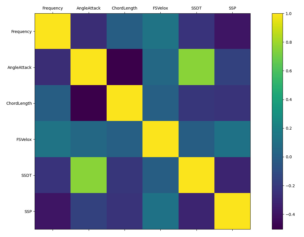
Figure 10.12: Correlogram of the DataFrame

As we already did in the case of the correlation matrix, in this case too, to analyze the correlation between predictors and the system response, it will be sufficient to consider the bottom row of the graph. The trends already obtained from the correlation matrix are confirmed.

Splitting the data

The training of an algorithm, based on machine learning, represents the crucial phase of the whole process of elaboration of the model. Performing the training of an ANN on the same dataset, which will subsequently be used to test the network, represents a methodological error. This is because the model will be able to perfectly predict the data used for testing, having already seen them in the training phase. However, when it will then be used to predict new cases that have never been seen before, it will inexorably commit evaluation errors. This problem is called data overfitting. To avoid this error, it is a good practice to train a neural network to use a different set of data from the one used in the test phase. Therefore, before proceeding with the training phase, it is recommended that you perform a correct division of the data.

Data splitting is used to split the original data into two sets: one is used to train a model and the other to test the model’s performance. The training and testing procedures represent the starting point for the model setting in predictive analytics. In a dataset that has 100 observations for predictor and response variables, a data splitting example occurs that divides this data into 70 rows for training and 30 rows for testing. To perform good data splitting, the observations must be selected randomly. When the training data is extracted, the data will be used to upload the weights and biases until an appropriate convergence is achieved.

The next step is to test the model. To do this, the remaining observations contained in the test set will be used to check whether the actual output matches the predicted output. To perform this check, several metrics can be adopted to validate the model:

1. We will use the sklearn library to split the ASNDataScaled DataFrame. To start, we will import the train_test_split function:

   from sklearn.model_selection import train_test_split
2. Now, we can divide the starting data into two sets: the X set containing the predictors and the Y set containing the target. We will use the pandas.DataFrame.drop() function, as follows:

   X = ASNDataScaled.drop('SSP', axis = 1)

   print('X shape = ',X.shape)

   Y = ASNDataScaled['SSP']

   print('Y shape = ',Y.shape)
3. Using the pandas.DataFrame.drop() function, we can remove rows or columns indicating label names and the corresponding axis or the index or column names. In this example, we have removed the target column (SSP) from the starting DataFrame.

The following shapes are printed:

X shape = (1503, 5)
Y shape = (1503,)

As is our intention, the two datasets, X and Y, now contain the five predictors and the system response, respectively.

4. Now we can divide the two datasets, X and Y, into two further datasets that will be used for the training phase and the test phase, respectively:

   X_train, X_test, Y_train, Y_test = train_test_split(X, Y, test_size = 0.30, random_state = 5)

   print('X train shape = ',X_train.shape)

   print('X test shape = ', X_test.shape)

   print('Y train shape = ', Y_train.shape)

   print('Y test shape = ',Y_test.shape)

The train_test_split() function was used by passing the following four parameters:

• X: The predictors.
• Y: The target.
• test_size: This parameter represents the proportion of the dataset to include in the test split. The following types are available: float, integer, or none, and optional (default = 0.25).
• random_state: This parameter sets the seed used by the random number generator. In this way, the repetitive splitting of the operation is guaranteed.

The following results are returned:

X train shape =  (1052, 5)
X test shape =  (451, 5)
Y train shape =  (1052,)
Y test shape =  (451,)

As expected, we finally divided the initial dataset into four subsets. The first two, X_train and Y_train, will be used in the training phase. The remaining two, X_test and Y_test, will be used in the testing phase.

Explaining multiple linear regression

In this section, we will deal with a regression problem using ANNs. To evaluate the results effectively, we will compare them with a model based on a different technology. Here, we will make a comparison between the model based on multiple linear regression and a model based on ANNs.

In multiple linear regression, the dependent variable (response) is related to two or more independent variables (predictors). The following equation is the general form of this model:

In the previous equation, x1, x2, ... xn are the predictors, and y is the response variable. The βi coefficients define the change in the response of the model related to the changes that occurred in xi, when the other variables remain constant. In the simple linear regression model, we are looking for a straight line that best fits the data. In the multiple linear regression model, we are looking for the plane that best fits the data. So, in the last one, our aim is to minimize the overall squared distance between this plane and the response variable.

To estimate the coefficients β, we want to minimize the following term:

To execute a multiple linear regression study, we can easily use the sklearn library. The sklearn.linear_model module is a module that contains several functions to resolve linear problems as a LinearRegression class that achieves an ordinary least squares linear regression:

1. To start, we will import the function as follows:

   from sklearn.linear_model import LinearRegression

Then, we set the model using the LinearRegression () function with the following command:

Lmodel = LinearRegression()

2. Now, we can use the fit() function to fit the model:

   Lmodel.fit(X_train, Y_train)

The following parameters are passed:

• X_train: The training data
• Y_train: The target data
• Eventually, a third parameter can be passed; this is the sample_weight parameter, which contains the individual weights for each sample

This function fits a linear model using a series of coefficients to minimize the residual sum of squares between the expected targets and the predicted targets predicted.

3. Finally, we can use the linear model to predict the new values using the predictors contained in the test dataset:

   Y_predLM = Lmodel.predict(X_test)

At this point, we have the predictions.

Now, we must carry out a first evaluation of the model to verify how much the prediction approached the expected value.

There are several descriptors for evaluating a prediction model. In this example, we will use the mean squared error (MSE).

Important note

MSE returns the average of the squares of the errors. This is the average squared difference between the expected values and the value that is predicted. MSE returns a measure of the quality of an estimator; this is a non-negative value and, the closer the values are to zero, the better the prediction.

4. To calculate the MSE, we will use the mean_squared_error() function contained in the sklearn.metrics module. This module contains score functions, performance metrics and pairwise metrics, and distance computations. We start by importing the function, as follows:

   from sklearn.metrics import mean_squared_error
5. Then, we can apply the function to the data:

   MseLM = mean_squared_error(Y_test, Y_predLM)

   print('MSE of Linear Regression Model')

   print(MseLM)
6. Two parameters were passed: the expected values (Y_test) and the values that were predicted (Y_predLM). Then, we print the results, as follows:

   MSE of Linear Regression Model

   0.015826467113949756

The value obtained is low and very close to zero. However, for now, we cannot add anything. We will use this value, later on, to compare it with the value that we calculate for the model based on neural networks.

Understanding a multilayer perceptron regressor model

A multilayer perceptron contains at least three layers of nodes: input nodes, hidden nodes, and output nodes. Apart from the input nodes, each node is a neuron that uses a nonlinear activation function. A multilayer perceptron works with a supervised learning technique and a backpropagation method for training the network. The presence of multiple layers and nonlinearity distinguish a multilayer perceptron from a simple perceptron. A multilayer perceptron is applied when data cannot be separated linearly:

1. To build a multilayer-perceptron-based model, we will use the sklearn MLPRegressor function. This regressor proceeds iteratively in the data training. At each step, it calculates the partial derivatives of the loss function with respect to the model parameters and uses the results obtained to update the parameters. There is a regularization term added to the loss function to reduce the model parameters to avoid data overfitting.

First, we will import the function:

from sklearn.neural_network import MLPRegressor

The MLPRegressor() function implements a multilayer perceptron regressor. This model optimizes the squared loss by using a limited-memory version of the Broyden–Fletcher–Goldfarb–Shanno (LBFGS) algorithm or stochastic gradient descent algorithm.

2. Now, we can set the model using the MLPRegressor function, as follows:

   MLPRegModel = MLPRegressor(hidden_layer_sizes=(50),

              activation='relu', solver='lbfgs',

              tol=1e-4, max_iter=10000, random_state=0)

The following parameters are passed:

• hidden_layer_sizes=(50): This parameter sets the number of neurons in the hidden layer; the default value is 100.
• activation='relu': This parameter sets the activation function. The following activation functions are available: identity, logistic, tanh, and ReLU. The last one is set by default.
• solver='lbfgs': This parameter sets the solver algorithm for weight optimization. The following solver algorithms are available: LBFGS, stochastic gradient descent (SGD), and the SGD optimizer (adam).
• tol=1e-4: This parameter sets the tolerance for optimization. By default, tol is equal to 1e-4.
• max_iter=10000: This parameter sets the maximum number of iterations. The solver algorithm iterates until convergence is imposed by tolerance or by this number of iterations.
• random_state=1: This parameter sets the seed used by the random number generator. In this way, it will be possible to reproduce the same model and obtain the same results.

3. After setting the parameters, we can use the data to train our model:

   MLPRegModel.fit(X_train, Y_train)

The fit () function fits the model using the training data for predictors (X_train) and the response (Y_train). Finally, we can use the model trained to predict new values:

Y_predMLPReg = MLPRegModel.predict(X_test)

In this case, the test dataset (X_test) was used.

4. Now, we will evaluate the performance of the MLP model using the MSE metric, as follows:

   MseMLP = mean_squared_error(Y_test, Y_predMLPReg)

   print(' MSE of the SKLearn Neural Network Model')

   print(MseMLP)

The following result is returned:

MSE of the SKLearn Neural Network Model
0.003315706807624097

At this point, we can make an initial comparison between the two models that we have set up: the multiple-linear-regression-based model and the ANN-based model. We will do this by comparing the results obtained by evaluating the MSE for the two models.

5. We obtained an MSE of 0.0158 for the multiple-linear-regression-based model, and an MSE of 0.0033 for the ANN-based model. The last one returns a smaller MSE than the first by an order of magnitude, confirming the prediction that we made where neural networks return values much closer to the expected values.

Finally, we make the same comparison between the two models; however, this time, we adopt a visual approach. We will draw two scatter plots in which we will report on the two axes the actual values (expected) and the predicted values, respectively:

# SKLearn Neural Network diagram
plt.figure(1)
plt.subplot(121)
plt.scatter(Y_test, Y_predMLPReg)
plt.plot((0, 1), "r--")
plt.xlabel("Actual values")
plt.ylabel("Predicted values")
plt.title("SKLearn Neural Network Model")
# SKLearn Linear Regression diagram
plt.subplot(122)
plt.scatter(Y_test, Y_predLM)
plt.plot((0, 1), "r--")
plt.xlabel("Actual values")
plt.ylabel("Predicted values")
plt.title("SKLearn Linear Regression Model")
plt.show()

By reporting the actual and expected values on the two axes, it is possible to check how this data is arranged. To help with the analysis, it is possible to trace the bisector of the quadrant, that is, the line of the equation, Y = X.

The following diagrams are printed:

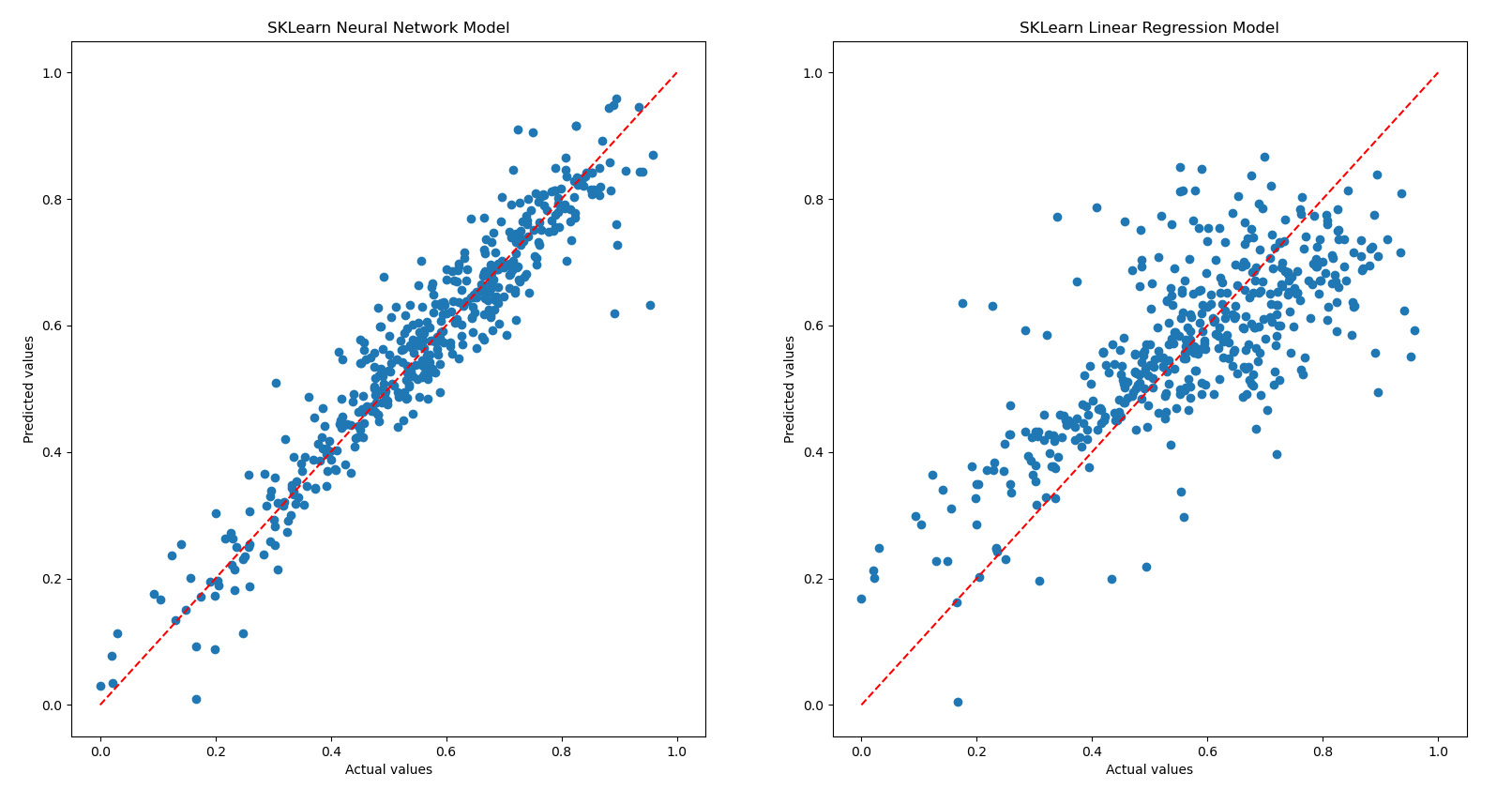
Figure 10.13: Scatterplots of the neural network models

Hypothetically, all observations should be positioned exactly on the bisector line (the dotted line in the diagram), but we can be satisfied when the data is close to this line. About half of the data points must be below the line and the other half must be above the line. Points that move significantly away from this line represent possible outliers.

Analyzing the results reported in the previous diagram, we can see that, in the graph related to the ANN-based model, the points are much closer to the dotted line. This confirms the idea that this model returns better predictions than the multiple-linear-regression-based model.

The recent history of ANNs has been enriched with models in which hidden layers extract information in different ways, in the next section we will explore deep learning.

Approaching deep neural networks

Deep learning is defined as a class of machine learning algorithms with certain characteristics. These models use multiple, hidden, nonlinear cascade layers to perform feature extraction and transformation jobs. Each level takes in the outputs from the previous level. These algorithms can be supervised, to deal with classification problems, or unsupervised, to deal with pattern analysis. The latter is based on multiple hierarchical layers of data characteristics and representations. In this way, the features of the higher layers are obtained from those of the lower layers, thus forming a hierarchy. Moreover, they learn multiple levels of representation corresponding to various levels of abstraction until they form a hierarchy of concepts.

The composition of each layer depends on the problem that needs to be solved. Deep learning techniques mainly adopt multiple hidden levels of an ANN but also sets of propositional formulas. The ANNs adopted have at least two hidden layers, but the applications of deep learning contain many more layers, for example, 10 or 20 hidden levels.

The development of deep learning in this period certainly depended on the exponential increase in data, with the consequent introduction of big data. In fact, with this exponential increase in data, there has been an increase in performance due to the increase in the level of learning, especially with respect to algorithms that already exist. In addition to this, the increase in computer performance also contributed to the improvement of obtainable results and to the considerable reduction in calculation times. There are several models based on deep learning. In the following sections, we will analyze the most popular ones.

Getting familiar with convolutional neural networks

A consequence of the application of deep learning algorithms to ANNs is the development of a new model that is much more complex but with amazing results, which is the convolutional neural network (CNN).

A CNN is a particular type of artificial feedforward neural network in which the connectivity pattern between neurons is inspired by the organization of the visual cortex of the human eye. Here, individual neurons are arranged in such a way as to devote themselves to the various regions that make up the visual field as a whole.

The hidden layers of this network are classified into various types: convolutional, pooling, ReLU, fully connected, and loss layers, depending on the role played. In the following sections, we will analyze them in detail.

Convolutional layers

This is the main layer of this model. It consists of a set of learning filters with a limited field of vision but extended along the entire surface of the input. Here, there are convolutions of each filter along the surface dimensions, making the scalar products between the filter inputs and the input image. Therefore, this generates a two-dimensional activation function that is activated if the network recognizes a certain pattern.

Pooling layers

In this layer, there is a nonlinear decimation that partitions the input image into a set of non-overlapping rectangles that are determined according to the nonlinear function. For example, with max pooling, the maximum of a certain value is identified for each region. The idea behind this layer is that the exact position of a feature is less important than its position compared to the others; therefore, superfluous information is omitted, also avoiding overfitting.

ReLU layers

The ReLU layer allows you to linearize the two-dimensional activation function and to set all negative values to zero.

Fully connected layers

This layer is generally placed at the end of the structure. It allows you to carry out the high-level reasoning of the neural network. It is called “fully connected” because the neurons in this layer have all been completely connected to the previous level.

Loss layers

This layer specifies how much the training penalizes the deviation between the predictions and the true values in output; therefore, it is always found at the end of the structure.

Examining recurrent neural networks

One of the tasks considered standard for a human, but of great difficulty for a machine, is the understanding of a piece of text. Given an ordered set of words, how can a machine be taught to understand its meaning? It is evident that, in this task, there is a more subtle relationship between the input data than in other cases. In the case of the process of classifying the content of an image, the whole image is processed by the machine simultaneously. This does not make sense in the elaboration of a piece of text, since the meaning of the words does not depend only on the words themselves, but also on their context.

Therefore, to understand a piece of text, it is not enough to know the set of words that are needed in it, it is necessary to relate them to respect the order in which they are read. It is necessary to consider, and subsequently remember, the temporal context.

Recurrent neural networks essentially allow us to remember data that could be significant during the process we want to study.

This depends on the propagation rule that is used. To understand the functioning of this type of propagation, and of memory, we can consider a case of a recurrent neural network: the Elman network.

An Elman network is very similar to a hidden single-layer feedforward neural network, but a set of neurons called context units is added to the hidden layer. For each neuron present in the hidden layer, a context unit is added, which receives, as input, the output of the corresponding hidden neuron and returns its output to the same hidden neuron.

A type of network very similar to that of Elman is that of Jordan, in which the context units save the states of the output neurons instead of those of the hidden neurons. The idea behind it, however, is the same as Elman, and it is the same as many other recurrent neural networks that are based on the following principle: receiving a sequence of data as input and processing a new sequence of output data, which is obtained by subsequently recalculating the data of the same neurons.

The recurrent neural networks that are based on this principle are manifold, and the individual topologies are chosen to face different problems. For example, in case it is not enough to remember the previous state of the network, but information processed many steps before may be necessary, long short-term memory (LSTM) neural networks can be used.

Analyzing long short-term memory networks

An LSTM is a special architecture of recurrent neural networks. These models are particularly suited to the context of deep learning because they offer excellent results and performance.

LSTM-based models are perfect for prediction and classification in the time series field, and they are replacing several traditional machine learning approaches. This is because LSTM networks can treat long-term dependencies between data. For example, this allows us to keep track of the context within a sentence to improve speech recognition.

An LSTM-based model contains cells, named LSTM blocks, which are linked together. Each cell provides three types of ports: the input gate, the output gate, and the forget gate. These ports execute the write, read, and reset functions, respectively, on the cell memory. These ports are analogical and are controlled by a sigmoid activation function in the range of 0–1. Here, 0 means total inhibition, and 1 means total activation. The ports allow the LSTM cells to remember information for an unspecified amount of time.

Therefore, if the input port reads a value below the activation threshold, the cell will maintain the previous state; whereas, if the value is above the activation threshold, the current state will be combined with the input value. The forget gate restores the current state of the cell when its value is zero, while the exit gate decides whether the value inside the cell should be removed or not.

Now let’s see a new technology developed using the ANNs, but this time, graph theory comes to the rescue.

Exploring GNNs

Using structured data as graphs in an ML model is problematic due to dimensionality and non-Euclidean properties. Researchers have tried to train ML models on graph-structured data by summarizing or representing information in a simplified way. But, this feels more like preprocessing than a real training process. GNNs help us create an end-to-end ML model trained to learn a representation of structured data in graphs and to fit a predictive model into it. In order to understand the operating principle of these algorithms, it is necessary to start from the basic concepts of graph theory.

Introducing graph theory

Graphs are rational mathematical structures that are used in various fields of study including mathematics, physics, and computer science up to topology, chemistry, and engineering. A graph is represented graphically by a structure of vertices and edges. The vertices can be seen as events from which different alternatives (the edge) start. Typically, graphics are used to represent a network in an unambiguous way: the vertices can represent PCs in a LAN, road junctions, or bus stops, while the edges can represent electrical connections or roads. Edges can connect vertices in any way possible. Graph theory is a branch of mathematics that allows us to describe sets of objects together with their relations; it was birthed in 1700 by Leonhard Euler.

A graph can be represented by the following equation:

In the previous formula, we can observe the following:

• V: set of vertices
• E: set of edges

A multigraph is a graph in which it is possible that the same pair of vertices is connected by several edges, while a hypergraph is a graph in which an edge can connect one or more vertices (even more than two).

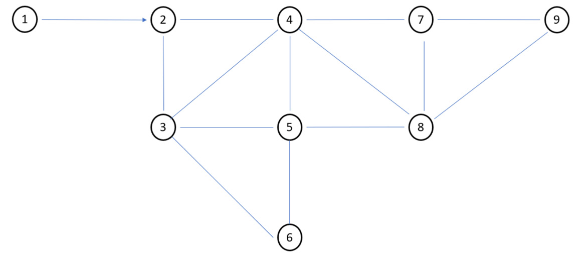
Figure 10.14: Visual representation of a graph

The number of vertices of the graph is the fundamental quantity to define its dimensions, while the number and distribution of edges describe its connectivity. Two vertices are said to be adjacent if they are connected by an arc. Adjacent edges are those edges that have a common vertex. There are several types of edges: direct edges and undirected edges without a direction. A direct edge is called an arc and its graph is called a digraph. For example, undirected edges are used to represent computer networks with synchronous links for data transmission while direct edges can represent road networks, allowing for the representation of two-way and one-way streets.

Connected graphs are defined as those for which we can reach all the other vertices of the graph from any vertex. Weighted graphs are defined as those for which a weight is associated with each arc, normally defined by a weight function (w). Weight can be seen as a cost or as the distance between the two nodes. The cost may depend on the flow that crosses the border through a law.

A vertex is characterized by its degree, which is equal to the number of edges that end on the vertex itself. According to the degree, the vertices are named as follows: isolated vertex if of order 0, leaf vertex if of order 1.

In an oriented graph, we can distinguish the outdegree (number of outgoing arcs), from the indegree (number of incoming arcs). Based on this hypothesis, the following vertices are named: source if it has zero degrees, sink if it has a degree greater than zero.

To represent a graph, we can adopt the visual representation that is obtained by drawing a point or a circle for each vertex and drawing a line between two vertices if they are connected to each other (Figure 10.14). If the edge is oriented, the direction is indicated by drawing an arrow.

Adjacency matrix

The graphical representation of a graph proposed in Figure 10.14 is very intuitive indeed, but it was a simple graph with only 9 vertices. What happens if, on the other hand, the leaders become centinaia? In this case, the graphical representation becomes confused, and it is convenient to adopt an alternative method: the adjacency matrix represents a suitable solution. The representation through the adjacency matrix of an undirected graph of n nodes and arcs occurs through a matrix A of size n × n where each row and each column correspond to the nodes and the elements of the aij matrix are equal to 0, if not there is an arc joining the two vertices (i and j), or they are equal to the sum of the number of edges joining the vertices (i and j). Obviously, if only one edge is allowed between two vertices, then the matrix will contain binary values (0 and 1).

The adjacency matrix for undirected graphs is symmetric and has n2 elements. Consequently, this representation is efficient only if the graph is significantly dense, while for sparse graphs there is a considerable waste of memory.

GNNs

GNNs learn from graph representation by extracting available information from graph elements and making it available in a low-dimensional space. Vertices collect information from their neighbors as they regularly exchange messages with each other. In this way, the information is transmitted and included in the properties of the respective vertex. The structural properties of the graph are iteratively englobed by aggregating information from the neighbors of each vertex. This procedure has an onerous computational cost and resampling can play a decisive role. The incorporation can be exploited by ML algorithms for classification or regression activities both at the top level and at the level of the entire graph. In the first case, the incorporation involves the representation of each vertex. In the second case, the grouping techniques are used for the incorporation.

In GNNs, the graph is processed by a set of units, one for each vertex, connected to each other according to the topology of the graph. Each unit calculates a status for the associated vertex, based on local information about the vertex and information about its neighbors. The state function is recursive and if the graph is cyclical, cyclical dependencies are also created in the connections of the neural network. One solution is to calculate the state through an iterative process, which will stop when an equilibrium point is reached. If the state function is a contraction mapping (that is, if it shortens the distances between points, but in a weaker way than a contraction), the system of equations admits a unique solution. Therefore, in order for the model to be applicable to a graph that is not direct or in any case containing cycles, it is necessary that constraints are imposed on the state function (that is, on the weights of the neural network) to ensure the contraction of the state function.

Let’s now analyze a practical application of using ANN-based models to simulate the behavior of materials.

Simulation modeling using neural network techniques

In this example, we will try to predict the quality of the concrete starting from its ingredients. Reinforced concrete, after about a century of life, has shown its vulnerability to the action of time, atmospheric agents, and earthquakes. The proportions of the phenomenon are such as to prevent any attempt at a solution based on the planned replacement of existing buildings; therefore, in recent years, the interest in the degradation and recovery of reinforced concrete structures has increased both to safeguard the existing building heritage and, when necessary, to increase the structural safety coefficients. The problem, already relevant in itself, immediately causes a second one, that of the correct design of new buildings, aimed at minimizing deterioration, avoiding, for the future, huge and unexpected recovery costs. All this is convincing the technicians that it is no longer enough to traditionally design concrete structures, based mainly on the mechanical verification of the sections. It is essential to spread a new concept of reinforced concrete, more complete and articulated, which leads to the choice of materials on the basis of durability and no longer only on resistance. In this perspective, a simulation model of the properties of the concrete starting from its basic constituents can represent an important resource to support the designer.

Concrete quality prediction model

Concrete is a mixture of binder (cement), water, and aggregates. In its fresh state, concrete has a plastic consistency, after laying and with time it hardens and, depending on the percentage quantity of the individual components, reaches lithoid characteristics, similar to those of a natural conglomerate. The mixture may also contain additives and mineral additions. Concrete can be classified either according to its characteristics or according to its composition. The mechanical characteristics of the concrete are evaluated through tests in the laboratory or in situ. Compressive strength is one of the most important characteristics of concrete. Based on the compressive strength, concrete can be classified into one of the classes provided. The evaluation is carried out on the basis of tests after 28 days on cylindrical specimens of 30 cm in length and 15 cm in diameter or cubic specimens with a side of 15 cm. Such tests are destructive, so having a tool that allows us to predict these characteristics is crucial.

In this section, we will elaborate on a model of prediction of the compressive strength of a concrete starting from the composition of the mixture of its constituents.

As always, we will analyze the code line by line:

1. Let’s start by importing the libraries and functions:

   import pandas as pd

   import seaborn as sns

   from sklearn.preprocessing import MinMaxScaler

   from sklearn.model_selection import train_test_split

   from keras.models import Sequential

   from keras.layers import Dense

   from sklearn.metrics import r2_score

The pandas library is an open source, BSD-licensed library that provides high-performance, easy-to-use data structures and data analysis tools for the Python programming language. It offers data structures and operations for manipulating numerical data in a simple way. In the seaborn module, there are several features we can use to graphically represent our data. There are methods that facilitate the construction of statistical graphs with matplotlib. The sklearn.preprocessing package provides several common utility functions and transformer classes to modify the features available in a representation that best suits our needs. The sklearn.model_selection.train_test_split() function computes a random split into training and test sets. We then imported the Keras models that we will use to build the ANN architecture. Finally, we imported the metrics for evaluating the network’s performance.

2. Now we need to import the data:

   features_names= ['Cement','BFS','FLA','Water','SP','CA','FA','Age','CCS']

   concrete_data = pd.read_excel('concrete_data.xlsx', names=features_names)

As we have already anticipated, our simulation will try to predict the compressive strength of the concrete starting from its basic components. To do this, we will use a dataset available on the UCI Machine Learning Repository at https://archive.ics.uci.edu/ml/datasets/concrete+compressive+strength. The dataset contains nine features: cement, blast furnace slag (BFS), fly ash (FLA), water, superplasticizer (SP), coarse aggregate (CA), fine aggregate (FA), age, and concrete compressive strength (CCS). The last feature is precisely the variable that we want to estimate. We, therefore, first defined the feature labels and then we used the pandas read_excel() function to import the file available in the .xlsx format.

3. So, let’s look at the statistics of the dataset:

   summary = concrete_data.describe()

   print(summary)

The following data is returned:

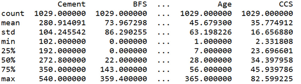
Figure 10.15: Summary of data

We can see that there are 1,029 records; moreover, the numerical values of the features have different ranges.

4. In order to better appreciate these differences, let’s draw a boxplot:

   sns.set(style="ticks")

   sns.boxplot(data = concrete_data)

The following chart is plotted:

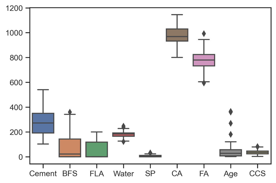
Figure 10.16: A boxplot of the features

As already mentioned, we can verify that the features have different ranges of values. This represents a factor that can be influential in the elaboration of a model based on ANNs: the variables that assume higher numerical values can assume a relevant weight in the prediction of the data, even if this is not true from the point of view of the phenomenon. In these cases, it is advisable to scale the data.

5. So, let’s try to scale the data:

   scaler = MinMaxScaler()

   print(scaler.fit(concrete_data))

   scaled_data = scaler.fit_transform(concrete_data)

   scaled_data = pd.DataFrame(scaled_data,

                        columns=features_names)

To do this, we used the MinMaxScaler () function of the sklearn.preprocessing library. The scaling is carried out using the following formula:

In this way, all features will have the same range of variability (0-1).

To confirm this, we proceed to carry out a new statistic on the scaled data:

summary = scaled_data.describe()
print(summary)

The following results are returned:

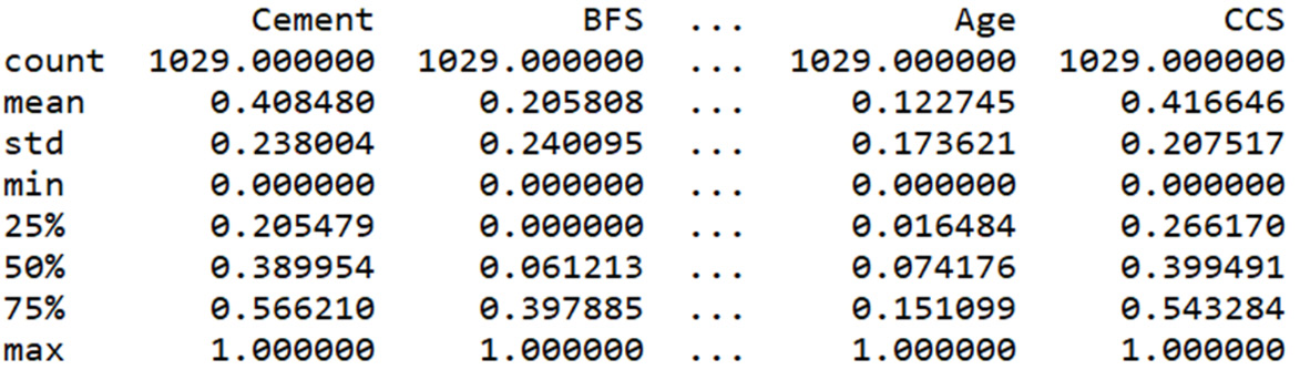
Figure 10.17: Statistics of the scaled features

6. Now each feature is scaled between 0–1. Let’s see the effect on the variables through the boxplot:

   sns.boxplot(data = scaled_data)

The following chart is plotted:

Figure 10.18: A boxplot of the scaled features

Now everything is clearer, we can easily make a visual check of the variability of the features in a much easier way. But above all, now we will not run the risk of introducing addictions to specific variables that are not true in reality.

7. Let’s reconstruct the pandas DataFrames for the input and output data:

   input_data = pd.DataFrame(scaled_data.iloc[:,:8])

   output_data = pd.DataFrame(scaled_data.iloc[:,8])
8. Now, we need to split the data we will use to train the model and test it:

   inp_train, inp_test, out_train, out_test = train_test_split(input_data,output_data, test_size = 0.30, random_state = 1)

   print(inp_train.shape)

   print(inp_test.shape)

   print(out_train.shape)

   print(out_test.shape)

Here, we used the train_test_split () function of the sklearn.model_selection library. This function quickly computes a random split into training and test sets. We decided to split the dataset into 70% for training and the remaining 30% to test the model. We also set the random_state to make the simulation reproducible. Finally, we printed the dimensions of the new datasets on the screen. The following values were printed:

(720, 8)
(309, 8)
(720, 1)
(309, 1) 

9. Now, we can build the ANN-based model:

   model = Sequential()

   model.add(Dense(20, input_dim=8, activation='relu'))

   model.add(Dense(10, activation='relu'))

   model.add(Dense(10, activation='relu'))

   model.add(Dense(1, activation='linear'))

   model.compile(optimizer='adam',loss='mean_squared_error',metrics=['accuracy'])

   model.fit(inp_train, out_train, epochs=1000, verbose=1)

The sequential class is used to define a linear stack of network layers that make up a model. The Dense class is used to instantiate a Dense layer, which is the basic feedforward fully connected layer. Fully connected levels are defined using the Dense class. The ANN architecture is a completely connected network structure with four layers (two hidden layers):

• The first layer added defines the input, three parameters are passed: 20, input_dim = 8, and activation = ' relu '. 20 (units) is a positive integer representing the dimensionality of the output space, denoting the number of neurons in the level. input_dim = 8 is the number of the input features. Finally, activation = ' relu ' is used to set the activation function (Rectified Linear Unit (ReLU) activation function.)
• The second layer (first hidden layer) has 10 neurons and the relu activation function
• The third layer (second hidden layer) has 10 neurons and the relu activation function, again
• Finally, the output layer has a single neuron (output) and a linear activation function.

10. Before training a model, we need to configure the learning process, which is done via the compile() method. Three arguments are passed: the adam optimizer, the mean_squared_error loss function, and the accuracy metric. The first parameter set the optimization as first-order gradient-based optimization of stochastic objective functions, based on adaptive estimates of lower-order moments. The second parameter measured the average of the squares of the errors. Finally, the third parameter set the evaluation metric as accuracy.

Finally, to train the model, the fit () method is used passing four arguments: the array of predictors training data, the array of response data, the number of epochs to train the model, and the verbosity mode.

Therefore, we summarize the characteristics of the model:

model.summary()

The following data is returned:

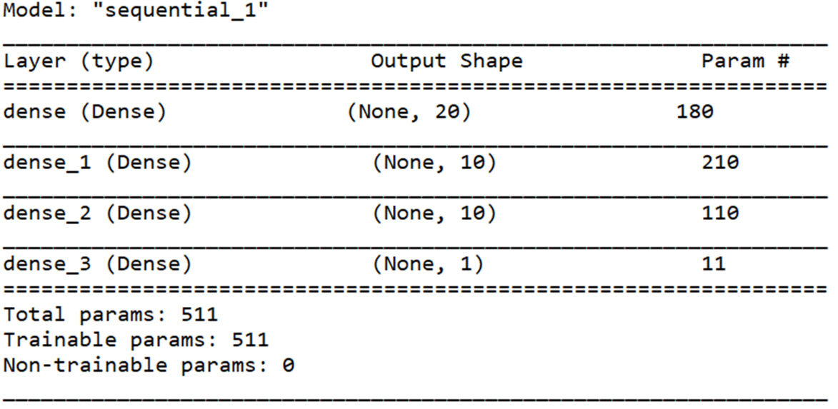
Figure 10.19: Architecture of ANN-based model

11. Now, we can finally use the model to make predictions of the characteristics of the material:

    output_pred = model.predict(inp_test)

We, therefore, predicted the compressive strength of the concrete starting from the mixture of ingredients.

12. Now, we just have to evaluate the performance of the model:

    print('Coefficient of determination = ')

    print(r2_score(out_test, output_pred))

To do this, we used the coefficient of determination. This metric indicates the proportion of total variance of the response values around its mean that is explained by the model. Precisely because it is a proportion, its value will always be between 0 and 1. The following result is returned:

Coefficient of determination = 
0.8591542120174626

We obtained a very high value to indicate the good predictive ability of the model.

Summary

In this chapter, we learned how to develop models based on ANNs to simulate physical phenomena. We started by analyzing the basic concepts of neural networks and the principles they are based on that are derived from biological neurons. We examined, in detail, the architecture of an ANN, understanding the concepts of weights, bias, layers, and the activation function.

Subsequently, we analyzed the architecture of a feedforward neural network. We saw how the training of the network with data takes place, and we understood the weight adjustment procedure that leads the network to correctly recognize new observations.

After that, we applied the concepts learned by tackling a practical case. We developed a model based on neural networks to solve a regression problem. We learned to scale data and then to subset the data for training and testing. We learned how to develop a model based on linear and MLP regression. We learned how to evaluate the performance of these models to make a comparison. Then, we explored deep neural networks. We defined them by analyzing their basic concepts. We analyzed the basics of CNNs, recurrent neural networks, and LSTM networks.

Finally, after introducing the theory of graphs and GNNs, we have faced a practical case of prediction of the physical characteristics of a material using the deep learning model.

In the next chapter, we will explore practical cases of project management using the tools we learned about in the previous chapters. We will learn how to evaluate the results of the actions we take when managing a forest using Markov processes, and then move on and learn how to evaluate a project using Monte Carlo simulation.