11

Modeling and Simulation for Project Management

Sometimes, monitoring resources, budgets, and milestones for various projects and divisions can present a challenge. Simulation tools help us to improve planning and coordination in the various phases of a project so that we always keep control of it. In addition, the preventive simulation of a project can highlight the critical issues related to a specific task. This helps us evaluate the cost of any actions to be taken. Through the preventive evaluation of the development of a project, errors that increase the costs of a project can be avoided.

In this chapter, we will deal with practical cases of project management using the tools we learned about in the previous chapters. We will learn how to evaluate the results of the actions we take when managing a forest using Markov processes, and then we will learn how to evaluate a project using the Monte Carlo simulation.

In this chapter, we’re going to cover the following main topics:

• Introducing project management
• Managing a tiny forest problem
• Scheduling project time using the Monte Carlo simulation

Technical requirements

In this chapter, we will address modeling examples of project management. To deal with these topics, it is necessary that you have a basic knowledge of algebra and mathematical modeling.

To work with the Python code in this chapter, you’ll need the following files (available on GitHub at the following URL: https://github.com/PacktPublishing/Hands-On-Simulation-Modeling-with-Python-Second-Edition):

• tiny_forest_management.py
• tiny_forest_management_modified.py
• monteCarlo_tasks_scheduling.py

Introducing project management

To assess the consequences of a strategic or tactical move in advance, companies need reliable predictive systems. Predictive analysis systems are based on data collection and the projection of reliable scenarios in the medium and long term. In this way, we can provide indications and guidelines for complex strategies, especially those that must consider numerous factors from different entities.

This allows us to examine the results of the evaluation in a more complete and coordinated way since we can simultaneously consider a range of values and, consequently, a range of possible scenarios. Finally, when managing complex projects, the use of artificial intelligence to interpret data has increased, thus giving these projects meaning. This is because we can perform sophisticated analyses of the information to improve the strategic decision-making process we will undertake. This methodology allows us to search and analyze data from different sources so that we can identify patterns and relationships that may be relevant.

Understanding what-if analysis

What-if analysis is a type of analysis that can contribute significantly to making managerial decisions more effective, safe, and informed. It is also the most basic level of predictive analysis that is based on data. What-if analysis is a tool capable of elaborating different scenarios to offer different possible outcomes. Unlike advanced predictive analysis, what-if analysis has the advantage of only requiring basic data to be processed.

This type of activity falls into the category of predictive analytics, that is, those that produce forecasts for the future, starting from a historical basis or trends. By varying some parameters, it is possible to simulate different scenarios and, therefore, understand what impact a given choice would have on costs, revenues, profits, and so on.

What-if analysis is therefore a structured method to determine which predictions related to strategy changes can go wrong, thereby judging the probability and consequences of the studies carried out before they happen. Through the analysis of historical data, it is possible to create such predictive systems capable of estimating future results following the assumptions that were made about a group of variables of independent inputs, thus allowing us to formulate some forecasting scenarios with the aim of evaluating the behavior of a real system.

Analyzing the scenario at hand allows us to determine the expected values related to a management project. These analysis scenarios can be applied in different ways, the most typical of which is to perform multi-factor analysis, that is, analyze models containing multiple variables:

• The realization of a fixed number of scenarios by determining the maximum and minimum difference and creating intermediate scenarios through risk analysis. Risk analysis aims to determine the probability that a future result will be different from the average expected result. To show this possible variation, an estimate of the less likely positive and negative results is performed.
• A random factorial analysis using Monte Carlo methods, thus solving a problem by generating appropriate random numbers and observing the fraction of the numbers that obey one or more properties. These methods are useful for obtaining numerical solutions for problems that are too complicated to solve analytically.

After having adequately introduced the basic concepts of project management, let’s now see how to implement a simple project by treating it as a Markovian process.

Managing a tiny forest problem

As we mentioned in Chapter 5, Simulation-Based Markov Decision Processes, a stochastic process is called Markovian if it starts from an instant t in which an observation of the system is made. The evolution of this process will depend only on t, so it will not be influenced by the previous instants. So, a process is called Markovian when the future evolution of the process depends only on that of instant of observing the system and does not depend in any way on the past. Markov Decision Processes (MDP) is characterized by five elements: decision epochs, states, actions, transition probability, and reward.

Summarizing the Markov decision process

The crucial elements of a Markovian process are the states in which the system finds itself and the available actions that the decision-maker can carry out in that state. These elements identify two sets: the set of states in which the system can be found, and the set of actions available for each specific state. The action chosen by the decision maker determines a random response from the system, which ultimately brings it into a new state. This transition returns a reward that the decision-maker can use to evaluate the efficacy of their choice.

Important note

In a Markovian process, the decision maker has the option of choosing which action to perform in each state of the system. The action chosen takes the system to the next state and the reward for that choice is returned. The transition from one state to another enjoys the property of Markov; the current state depends only on the previous one.

A Markov process is defined by four elements, as follows:

• S: System states
• A: Actions available for each state
• P: Transition matrix. This contains the probabilities that an action a takes the system from s state to s’ state
• R: Rewards obtained in the transition from s state to s’ state with an action a

In an MDP problem, it becomes crucial to take action to obtain the maximum reward from the system. Therefore, this is an optimization problem in which the sequence of choices that the decision-maker will have to make is called an optimal policy.

A policy maps both the states of the environment and the actions to be chosen for those states, representing a set of rules or associations that respond to a stimulus. The policy’s goal is to maximize the total reward received through the entire sequence of actions performed by the system. The total reward that’s obtained by adopting a policy is calculated as follows:

In the previous equation, rT is the reward of the action that brings the environment into the terminal state sT. To get the maximum total reward, we can select the action that provides the highest reward to each individual state. This leads to us choosing the optimal policy that maximizes the total reward.

Exploring the optimization process

As we mentioned in Chapter 5, Simulation-Based Markov Decision Processes, an MDP problem can be addressed using dynamic programming (DP). DP is a programming technique that aims to calculate an optimal policy based on a knowing model of the environment. The core of DP is to utilize the state value and action value to identify good policies.

In DP methods, two processes called policy evaluation and policy improvement are used. These processes interact with each other, as follows:

• Policy evaluation is done through an iterative process that seeks to solve Bellman’s equation. The convergence of the process for k → ∞ imposes approximation rules, thus introducing a stop condition.
• Policy improvement improves the current policy based on the current values.

In the DP technique, the previous phases alternate and end before the other begins via an iteration procedure. This procedure requires a policy evaluation at each step, which is done through an iterative method, whose convergence is not known a priori and depends on the starting policy; that is, we can stop evaluating the policy at some point, while still ensuring convergence to an optimal value.

Important note

The iterative procedure we have described uses two vectors that preserve the results obtained from the policy evaluation and policy improvement processes. We indicate the vector that will contain the value function with V, that is, the discounted sum of the rewards obtained. We indicate the carrier that will contain the actions chosen to obtain those rewards with Policy.

The algorithm then, through a recursive procedure, updates these two vectors. In the policy evaluation, the value function is updated as follows:

In the previous equation, we have the following:

• is the function value at the state s
• is the reward returned in the transition from state s to state s’
• γ is the discount factor
• is the function value at the next state

In the policy improvement process, the policy is updated as follows:

In the previous equation, we have the following:

• is the function value at state s’
• is the reward returned in the transition from state s to state s’ with action a
• γ is the discount factor
• is the probability that an action a in the s state is carried out in the s’ state

Now, let’s see what tools we have available to deal with MDP problems in Python.

Introducing MDPtoolbox

The MDPtoolbox package contains several functions connected to the resolution of discrete-time Markov decision processes, such as value iteration, finite horizon, policy iteration, linear programming algorithms with some variants, and several functions we can use to perform reinforcement learning analysis.

This toolbox was created by researchers from the Applied Mathematics and Computer Science Unit of INRA Toulouse (France), in the MATLAB environment. The toolbox was presented by the authors in the following article: Chadès, I., Chapron, G., Cros, M. J., Garcia, F., & Sabbadin, R. (2014). MDPtoolbox: a multi-platform toolbox to solve stochastic dynamic programming problems. Ecography, 37 (9), 916-920.

Important note

The MDPtoolbox package was subsequently made available in other programming platforms, including GNU Octave, Scilab, and R. It was later made available for Python programmers by S. Cordwell.

You can find out more at the following URL: https://github.com/sawcordwell/pymdptoolbox.

To use the MDPtoolbox package, we need to install it. The different installation procedures are indicated on the project’s GitHub website. As recommended by the author, you can use the default Python pip package manager. Python Package Index (pip) is the largest and most official Python package repository. Anyone who develops a Python package, in 99% of cases, makes it available on this repository.

To install the MDPtoolbox package using pip, just write the following command:

pip install pymdptoolbox

Once installed, just load the library to be able to use it immediately.

Defining the tiny forest management example

To analyze in detail how to deal with a management problem using Markovian processes, we will use an example already available in the MDPtoolbox package. It deals with managing a small forest in which there are two types of resources: wild fauna and trees. The trees of the forest can be cut, and the wood that’s obtained can be sold. The decision maker has two actions: wait and cut. The first action is to wait for the tree to grow fully before cutting it to obtain more wood. The second action involves cutting the tree to get money immediately. The decision maker has the task of making their decision every 20 years.

The tiny forest environment can be in one of the following three states:

• State 1: Forest age 0-20 years
• State 2: Forest age 21-40 years
• State 3: Forest age over 40 years

We might think that the best action is to wait until we have the maximum amount of wood to come and thus obtain the greatest gain. Waiting can lead to the loss of all the wood available. This is because as the trees grow, there is also the danger that a fire could develop, which could cause the wood to be lost completely. In this case, the tiny forest would be returned to its initial state (state 1), so we would lose what we would have gained by waiting until the forest reached full maturity (state 3).

In the case a fire does not occur, at the end of each period t (20 years), if the state is s and the wait action is chosen, the forest will move to the next state, which will be the minimum of the following pair (s + 1, 3). If there are no fires, the age of the forest will never assume a state higher than 3, since state 3 matches the oldest age class. Conversely, if a fire occurs after the action is applied, the forest returns the system to its initial state (state 1), as shown in the following figure:

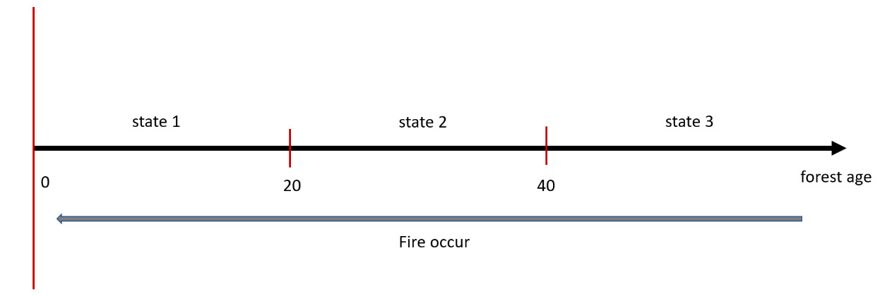
Figure 11.1 – States of the age of a forest

Set P = 0.1 as the probability that a fire occurs during a period t: the problem is how to manage this in the long term to maximize the reward. This problem can be treated as a Markov decision process.

Now, let’s move on and define the problem as an MDP. We have said that the elements of an MDP are state, action, transition matrix (P), and reward (R). We must then define these elements. We have defined the states already – there are three. We also defined the actions, which are wait or cut. We pass these to define the transition matrix P (s, s’, a). It contains the chances of the system going from one state to another. We have two actions available (wait or cut), so we will define two transition matrices. If we indicate with p the probability that a fire occurs, then in the case of the wait action, we will have the following transition matrix:

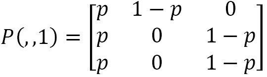
Now, let’s analyze the content of the transition matrix. Each row is relative to a state, in the sense that row 1 returns the probabilities that, starting from state 1, the tiny forest will remain in state 1 or pass to state 2 or 3. If we are in state 1, we will have a probability p that the tiny forest will remain in that state, which happens if a fire occurs. Beginning in state 1, if no fire occurs, we have the remaining 1-p probability of moving to the next state, which is state 2. When starting from state 1, the probability of passing to state 3 is equal to 0 – it’s impossible to do so.

Row 2 of the transition matrix contains the transition probabilities when starting from state 2. If a fire occurs when starting from state 2, there will be an equal probability p to pass into state 1. If no fire occurs when starting from state 2, we have the remaining 1-p probability of moving to the next state, which is state 3. In this case, once again, the probability of remaining in state 2 is equal to 0.

To better understand the transition of states we can analyze the transition diagram first introduced in Chapter 5, Simulation-Based Markov Decision Processes (Figure 11.2).

Figure 11.2 – Transition diagram

Finally, if we are in state 3 and a fire occurs, we will have a probability equal to p that we will go back to state 1, and the remaining 1-p probability of remaining in state 3, which happens if no fire occurs. The probability of going to state 2 is equal to 0.

Now, let’s define the transition matrix in the case of choosing the cut action:

In this case, the analysis of the previous transition matrix is much more immediate. In fact, the cut action brings the state of the system to 1 in each instance. Therefore, the probability is always 1. Then, that 1 goes to state 1 and 0 for all the other transitions as they are not possible.

Now, let’s define the vectors that contain the rewards, that is, the vector R (s, s’, as we have defined it), starting from the rewards returned by the wait action:

The action of waiting for the growth of the forest will bring a reward of 0 for the first two states, while the reward will be the maximum for state 3. The value of the reward in state 3 is equal to 4, which represents the value provided by the system by default. Let’s see how the vector of rewards is modified if you choose the cut action:

In this case, cutting in state 1 does not bring any reward since the trees are not able to supply wood yet. The decision to cut the trees in state 2 brings a reward, but this is lower than the maximum one, which is obtainable if we wait for the end of the three periods t before cutting. A similar situation arises if the cut is made at the beginning of the third period. In this case, the reward is greater than that of the previous state but still less than the maximum.

Addressing management problems using MDPtoolbox

Our goal is to develop a policy that allows us to manage the tiny forest to obtain the maximum prize. We will do this using the MDPtoolbox package, which we introduced in the previous section, and analyzing the code line by line:

1. Let’s start as always by importing the necessary library:

   import mdptoolbox.example

By doing this, we imported the MDPtoolbox module, which contains the data for this example.

2. To begin, we will extract the transition matrix and the reward vectors:

   P, R = mdptoolbox.example.forest()

This command retrieves the data stored in the example. To confirm the data is correct, we need to print the content of these variables, starting from the transition matrix:

print(P[0])

The following matrix is printed:

[[0.1 0.9 0. ]
 [0.1 0.  0.9]
 [0.1 0.  0.9]]

This is the transition matrix for the wait action. Consistent with what is indicated in the Defining the tiny forest management example section, after having set p = 0.1 we can confirm the transition matrix.

3. Now, we will print the transition matrix related to the cut action:

   print(P[1])

The following matrix is printed:

[[1. 0. 0.]
 [1. 0. 0.]
 [1. 0. 0.]]

4. This matrix is also consistent with what was previously defined. Now, let’s check the shape of the reward vectors, starting from the wait action:

   print(R[:,0])

Let’s see the content of this vector:

[0. 0. 4.]

If the cut action is chosen, we will have the following rewards:

print(R[:,1])

The following vector is printed:

[0. 1. 2.]

5. Finally, let’s fix the discount factor:

   gamma=0.9

All the problem data has now been defined. We can now move on and look at the model in greater detail.

6. The time has come to apply the policy iteration algorithm to the problem we have just defined:

   PolIterModel = mdptoolbox.mdp.PolicyIteration(P, R, gamma)

   PolIterModel.run()

The mdptoolbox.mdp.PolicyIteration() function performs a discounted MDP that’s solved using the policy iteration algorithm. Policy iteration is a dynamic programming method that adopts a value function in order to model the expected return for each pair of action-state. These techniques update the value functions by using the immediate reward and the (discounted) value of the next state in a process called bootstrapping. The results are stored in tables or with approximate function techniques.

The function, starting from an initial P0 policy, updated the function value and the policy through an iterative procedure, alternating the following two phases:

• Policy evaluation: Given the current policy P, estimate the action-value function.
• Policy Improvement: If we calculate a better policy based on the action-value function, then this policy is made the new policy and we return to the previous step.

When the value function can be calculated exactly for each action-state pair, the policy iteration we performed with the greedy policy improvement leads to convergence by returning the optimal policy. Essentially, repeatedly executing these two processes converges the general process toward the optimal solution.

In the mdptoolbox.mdp.PolicyIteration() function, we have passed the following arguments:

• P: Transition probability
• R: Reward
• gamma: Discount factor

The following results are returned:

• V: The optimal value function. V is an S length vector.
• Policy: The optimal policy. The policy is an S length vector. Each element is an integer corresponding to an action that maximizes the value function. In this example, only two actions are foreseen: 0 = wait, and 1 = cut.
• iter: The number of iterations.
• time: The CPU time used to run the program.

7. Now that the model is ready, we must evaluate the results by checking the obtained policy.

To begin, we will check the updates of the value function:

print(PolIterModel.V)

The following results are returned:

(26.244000000000014, 29.484000000000016, 33.484000000000016)

A value function specifies how good a state is for the system. This value represents the total reward expected for a system from the status s. The value function depends on the policy that the agent selects for the actions to be performed.

8. Let’s move on and extract the policy:

   print(PolIterModel.policy)

A policy suggests the behavior of the system at a given time. It maps the detected states of the environment and the actions to take when they are in those states. This corresponds to what, in psychology, would be called a set of rules or associations of the stimulus-response. The policy is the crucial element of an MDP model since it defines the behavior. The following results are returned:

(0, 0, 0)

Here, the optimal policy is to not cut the forest in all three states. This is due to the low probability of a fire occurring, which causes the wait action to be the best action to perform. In this way, the forest has time to grow and we can achieve both goals: maintain an old forest for wildlife and earn money by selling the cut wood.

9. Let’s see how many iterations have been made:

   print(PolIterModel.iter)

The following result is returned:

2

10. Finally, let’s print the CPU time:

    print(PolIterModel.time)

The following result is returned:

0.0009965896606445312

Only 0.0009 seconds are required to perform the value iteration procedure, but obviously, this value depends on the machine in use.

Changing the probability of a fire starting

The analysis of the previous example has clarified how to derive an optimal policy from a well-posed problem. We can now define a new problem by changing the initial conditions of the system. Under the default conditions provided in our example, the probability of a fire occurring is low. In this case, we have seen that the optimal policy advises us to wait and not cut the forest. But what if we increase the probability of a fire occurring? This is a real-life situation; just think of warm places particularly subject to strong winds. To model this new condition, simply change the problem settings by changing the probability value p. The mdptoolbox.example.forest() module allows us to modify the basic characteristics of the problem. Let’s get started:

1. Let’s start by importing the example module:

   import mdptoolbox.example

   P, R = mdptoolbox.example.forest(3,4,2,0.8)

Compared to the example discussed in the previous section, Addressing management problems using MDPtoolbox, we have passed some parameters. Let’s analyze them in detail.

In the mdptoolbox.example.forest () function, we passed the following parameters (3, 4, 2, 0.8).

Let’s analyze their meaning:

• 3: The number of states. This must be an integer greater than 0.
• 4: The reward when the forest is in the oldest state and the wait action is performed. This must be an integer greater than 0.
• 2: The reward when the forest is in the oldest state and the cut action is performed. This must be an integer greater than 0.
• 0.8: The probability of a fire occurring. This must be in [0, 1].

By analyzing the past data, we can see that we confirmed the first three parameters, while we only changed the probability of a fire occurring, thus increasing this possibility from 0.1 to 0.8.

2. Let’s see this change to the initial data as it changed the transition matrix:

   print(P[0])

The following matrix is printed:

[[0.8 0.2 0. ]
 [0.8 0.  0.2]
 [0.8 0.  0.2]]

As we can see, the transition matrix linked to the wait action has changed. Now, the probability that the transition is in a state other than 1 has significantly decreased. This is due to the high probability that a fire will occur. Let’s see what happens when the transition matrix is linked to the cut action:

print(P[1])

The following matrix is printed:

[[1. 0. 0.]
 [1. 0. 0.]
 [1. 0. 0.]]

This matrix remains unchanged. This is due to the cut action, which returns the system to its initial state. Likewise, the reward vectors may be unchanged since the rewards that were passed are the same as the ones provided by the default problem. Let’s print these values:

print(R[:,0])

This is the reward vector connected to the wait action. The following vector is printed:

[0. 0. 4.]

In the case of the cut action, the following vector is returned:

print(R[:,1])

The following vector is printed:

[0. 1. 2.]

As anticipated, nothing has changed. Finally, let’s fix the discount factor:

gamma=0.9

All the problem data has now been defined. We can now move on and look at the model in greater detail.

3. We will now apply the value iteration algorithm:

   PolIterModel = mdptoolbox.mdp.PolicyIteration(P, R, gamma)

   PolIterModel.run()
4. Now, we can extract the results, starting from the value function:

   print(PolIterModel.V)

The following results are printed:

(1.5254237288135597, 2.3728813559322037, 6.217445225299711)

5. Let’s now analyze the crucial part of the problem: let’s see what policy the simulation model suggests:

   print(PolIterModel.policy)

The following results are printed:

(0, 1, 0)

In this case, the changes we’ve made here, compared to the default example, are substantial. It’s suggested that we adopt the wait action if we are in state 1 or 3, while if we are in state 2, it is advisable to try to cut the forest. Since the probability of a fire is high, it is convenient to cut the wood already available and sell it before a fire destroys it.

6. Then, we print the number of iterations of the problem:

   print(PolIterModel.iter)

The following result is printed:

1

Finally, we print the CPU time, which is as follows:

print(PolIterModel.time)

The following result is printed:

0.0009970664978027344

These examples have highlighted how simple the modeling procedure of a management problem is through using MDPs.

Now, let’s see how to design a scheduling grid using the Monte Carlo simulation.

Scheduling project time using the Monte Carlo simulation

Each project requires a time of realization, and the beginning of some activities can be independent or dependent on previous activities ending. Scheduling a project means determining the time of realization for the project itself. A project is a temporary effort undertaken to create a unique product, service, or result. The term project management refers to the application of knowledge, skills, tools, and techniques for the purpose of planning, managing, and controlling a project and the activities that it is composed of.

The key figure in this area is the project manager, who has the task and responsibility of coordinating and controlling the various components and actors involved in the project, with the aim of reducing the probability of project failure. The main difficulty in this series of activities is achieving the objectives set in compliance with any constraints, such as the scope of the project, time, costs, quality, and resources. In fact, these are limited aspects that are linked to each other and need effective optimization.

The definition of these activities constitutes one of the key moments of the planning phase. After defining what the project objectives are with respect to time, costs, and resources, it is necessary to proceed with identifying and documenting the activities that must be carried out to successfully complete the project.

For complex projects, it is necessary to create an ordered structure by decomposing the project into simpler tasks. For each task, it will be necessary to define the activities and their execution times. This starts with the main objective and breaks down the project to the immediately lower level in all those deliverables or main sub-projects that make it up.

These will, in turn, be broken down. This will continue until you are satisfied with the degree of detail in the resulting final items. Each breakdown results in a reduction in the size, complexity, and cost of the interested party.

Defining the scheduling grid

A fundamental part of project management is constructing the scheduling grid. This is an oriented graph that represents the temporal succession and the logical dependencies between the activities that are involved in the realization of the project. In addition to constructing the grid, the scheduling process also determines the start and end times of the activities based on factors such as duration, resources, and so on.

In the example we are dealing with, we will evaluate the times necessary for the realization of a complex project. Let’s start by defining the scheduling grid. Suppose that, by decomposing the project structure, we have defined six tasks. For each task, the activities, the personnel involved, and the time needed to finish the job were defined.

Some tasks must be performed in a series, in the sense that the activities of the previous task must be completed so that they can start the activities of the next task. Others, however, can be performed in parallel, in the sense that two teams can simultaneously work on two different tasks to reduce project delivery times. This sequence of tasks is defined in the scheduling grid, as follows:

Figure 11.3 – The sequence of tasks in the grid

The preceding diagram shows us that the first two tasks developed in parallel, which means that the time required to finish these two tasks will be provided by the time-consuming task. The third task develops in a series, while the next two are, again, in parallel. The last task is still in the series. This sequence will be necessary when we evaluate the project times.

Estimating the task’s time

The duration of these tasks is often difficult to estimate due to the number of factors that can influence it such as the availability and/or productivity of the resources, the technical and physical constraints between the activities, and the contractual commitments.

Expert advice, supported by historical information, can be used wherever possible. The members of the project team will also be able to provide information on the duration of the task or the maximum recommended limit for the duration of the task by deriving information from similar projects.

There are several ways we can estimate tasks. In this example, we will use a three-point estimation. In a three-point estimation, the accuracy of the duration of the activity estimate can be increased in terms of the amount of risk in the original estimate. Three-point estimates are based on determining the following three types of estimates:

• Optimistic: The duration of the activity is based on the best scenario of what is described in the most probable estimate. This is the minimum time it will take to complete the task.
• Pessimistic: The duration of the activity is based on the worst-case scenario of what is described in the most probable estimate. This is the maximum time that it will take to complete the task.
• More likely: The duration of the activity is based on realistic expectations in terms of availability for the planned activity.

A first estimate of the duration of the activity can be constructed using an average of the three estimated durations. This average typically provides a more accurate estimate of the duration of the activity than a more likely single-value estimate. But that’s not what we want to do.

Suppose that the project team used three-point estimation for each of the six tasks. The following table shows the times proposed by the team:

Table 11.1– A time chart for individual tasks

After defining the sequence of tasks and the time it will take to perform each individual task, we can develop an algorithm for estimating the overall time of the project.

Developing an algorithm for project scheduling

In this section, we will analyze an algorithm for scheduling a project based on Monte Carlo simulation. We will look at all the commands in detail, line by line:

1. Let’s start by importing the libraries that we will be using in the algorithm:

   import numpy as np

   import random

   import pandas as pd

numpy is a Python library that contains numerous functions that help us manage multidimensional matrices. Furthermore, it contains a large collection of high-level mathematical functions we can use on these matrices.

The random library implements pseudo-random number generators for various distributions. The random module is based on the Mersenne Twister algorithm.

The pandas library is an open source BSD licensed library that contains data structures and operations that can be used to manipulate high-performance numeric values for the Python programming language.

2. Let’s move on and initialize the parameters and the variables:

   N = 10000

   TotalTime=[]

   T =  np.empty(shape=(N,6)) 

N represents the number of points that we generate. These are the random numbers that will help us define the time for that task. The TotalTime variable is a list that will contain the N assessments of the overall time needed to complete the project. Finally, the T variable is a matrix with N rows and six columns and will contain the N assessments of the time needed to complete each individual task.

3. Now, let’s set the three-point estimation matrix, as defined in the table in the Estimating the task’s time section:

   TaskTimes=[[3,5,8],

              [2,4,7],

              [3,5,9],

              [4,6,10],

              [3,5,9],

              [2,6,8]]

This matrix contains the three times for each representative row of the six tasks: optimistic, more likely, and pessimistic.

At this point, we must establish the form of the distribution for the times that we intend to adopt.

Exploring triangular distribution

When developing a simulation model, it is necessary to introduce probabilistic events. Often, the simulation process starts before you have enough information about the behavior of the input data. This forces us to decide on a distribution. Among those that apply to incomplete data is the triangular distribution. The triangular distribution is used when assumptions can be made about the minimum, maximum, and modal values.

Important note

A probability distribution is a mathematical model that links the values of a variable to the probabilities that these values can be observed. Probability distributions are used for modeling the behavior of a phenomenon of interest in relation to the reference population, or to all the cases in which the investigator observes a given sample.

In Chapter 3, Probability and Data Generating Processes, we analyzed the most widely used probability distributions. When the random variable is defined in a certain range, but there are reasons to believe that the degrees of confidence decreases linearly from the center to the extremes, there is the so-called triangular distribution. This distribution is very useful for calculating measurement uncertainties since, in many circumstances, this type of model can be more realistic than the uniform one.

The triangular distribution is a continuous probability distribution whose probability density function describes a triangle, returning a null distribution on the two extreme values and linearly between those extreme values and an intermediate value, which represents its mode as seen in Figure 11.4. It is used as a model when the sample available is very small, estimating the minimum, maximum, and fashion values.

Let’s consider the first task of the project we are analyzing. For this, we have defined the three times estimated for the project: optimistic (3), more likely (5), and pessimistic (8). We can draw a graph in which we report these estimates three times on the abscissa and the probability of their occurrence on the ordinate. Using the triangular probability distribution, the probability that the event occurs is between the limit values, which, in our case, are optimistic and pessimistic. We do this while assuming the maximum value in correspondence with the value more likely to occur. For the intermediate values, where we know nothing, suppose that the probability increases linearly from optimistic to more likely, and then always decreases linearly from more likely to pessimistic, as shown in the following graph:

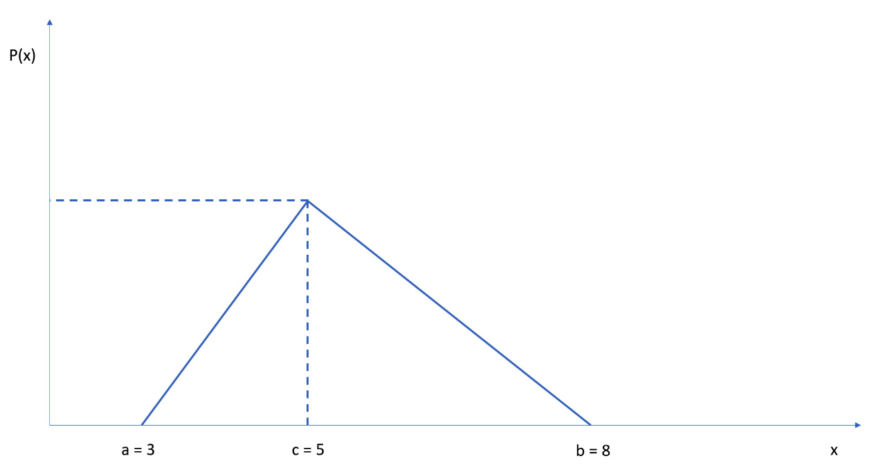
Figure 11.4 – Probability graph

Our goal is to model the times of each individual task using a random variable with uniform distribution in the interval (0, 1). If we indicate this random variable with trand, then the triangular distribution allows us to evaluate the probability that the task ends in that time is distributed. In the triangular distribution, we have identified two triangles that have the abscissa in common for x = c. This value acts as a separator between the two values that the distribution assumes. Let’s denote it with Lh. The value is given the following formula:

In the previous equation, we have the following:

• a: The optimistic time
• b: The pessimistic time
• c: The more likely time

That being said, we can generate variations according to the triangular distribution with the following equations:

The previous equations allow us to perform the Monte Carlo simulation. Let’s see how we can do this:

1. First, we generate the separation value of the triangular distribution:

   Lh=[]

   for i in range(6):

       Lh.append((TaskTimes[i][1]-TaskTimes[i][0])

                /(TaskTimes[i][2]-TaskTimes[i][0]))

Here, we initialized a list and then populated it with a for loop that iterates over the six tasks, evaluating a value of Lh for each one.

2. Now, we can use two for loops and an if conditional structure to develop the Monte Carlo simulation:

   for p in range(N):

       for i in range(6):

           trand=random.random()

           if (trand < Lh[i]):

               T[p][i] = TaskTimes[i][0] + 

                      np.sqrt(trand*(TaskTimes[i][1]-  

                      TaskTimes[i][0])*

                      (TaskTimes[i][2]-TaskTimes[i][0]))

           else:

               T[p][i] = TaskTimes[i][2] – 

                      np.sqrt((1-trand)*(TaskTimes[i][2]-

                      TaskTimes[i][1])*

                     (TaskTimes[i][2]-TaskTimes[i][0]))

The first for loop continues generating the random values N times, while the second loop is used to perform the evaluation for six tasks. The conditional if structure, on the other hand, is used to discriminate between the two values distinct from the value of Lh so that it can use the two equations that we defined previously.

3. Finally, for each of the N iterations, we calculate an estimate of the total time for the execution of the project:

   TotalTime.append( T[p][0]+        

                    np.maximum(T[p][1],T[p][2]) + 

                    np.maximum(T[p][3],T[p][4]) + T[p][5])

For the calculation of the total time, we referred to the scheduling grid defined in the Defining the scheduling grid section. The procedure is simple: if the tasks develop in a series, then you add the times up, while if they develop in parallel, you choose the maximum value among the times of the tasks.

4. Now, let’s take a look at the values we have attained:

   Data = pd.DataFrame(T,columns=[‘Task1’, ‘Task2’, ‘Task3’, 

                                 ‘Task4’, ‘Task5’, ‘Task6’])

   pd.set_option(‘display.max_columns’, None)  

   print(Data.describe())

For detailed statistics of the times estimated with the Monte Carlo method, we have transformed the matrix (Nx6) containing the times into a pandas DataFrame. The reason for this is that the pandas library has useful functions that allow us to extract detailed statistics from a dataset immediately. In fact, we can do this with just a line of code by using the describe() function.

The describe() function generates a series of descriptive statistics that return useful information on the dispersion and the form of the distribution of a dataset.

The pandas set.option() function was used to display all the statistics of the matrix and not just a part of it, as expected by default.

The following results are returned:

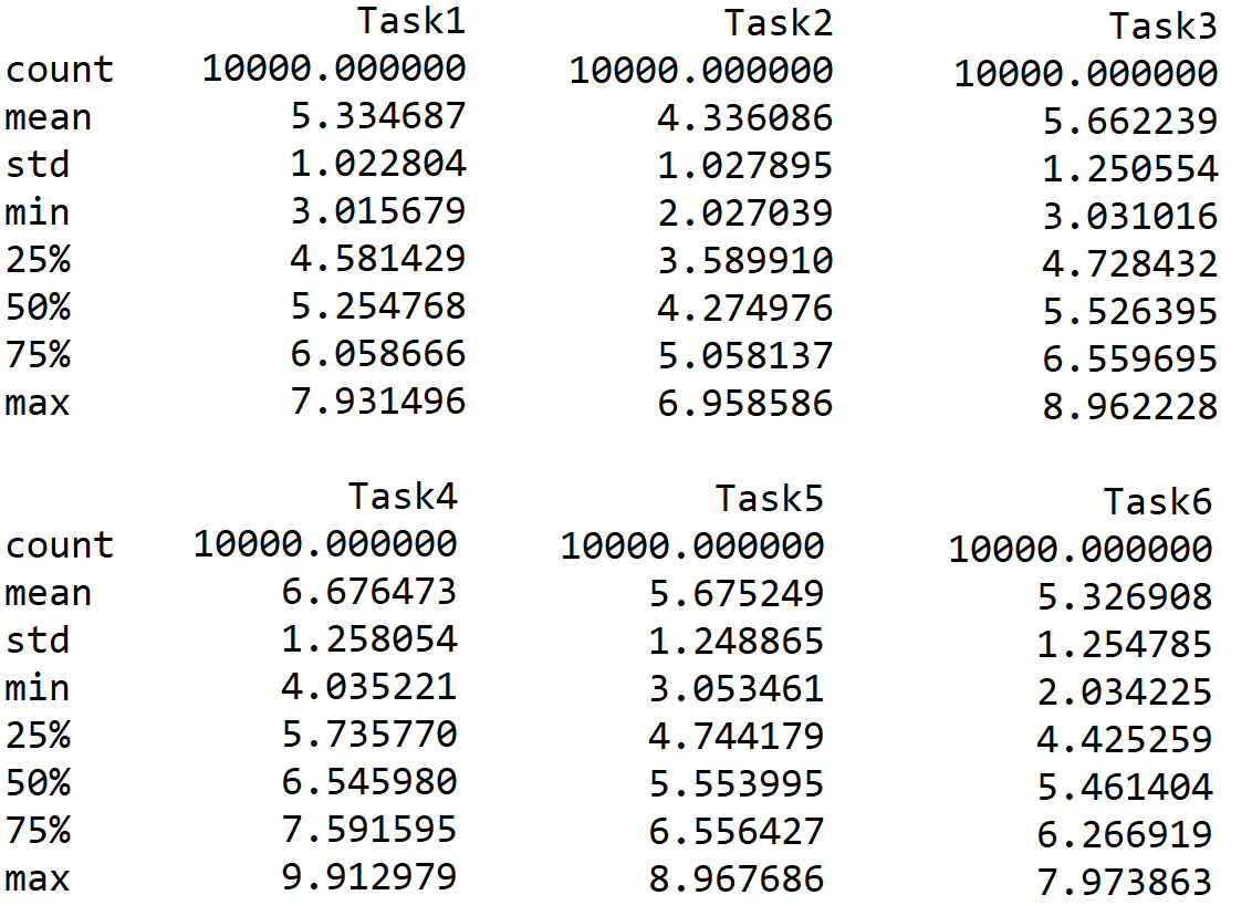
Figure 11.5 – The values of the DataFrame

By analyzing these statistics, we have confirmed that the estimated times are between the limit values imposed by the problem: optimistic and pessimistic. In fact, the minimum and maximum times are very close to these values. Furthermore, we can see that the standard deviation is very close to the unit. Finally, we can confirm that we have generated 10,000 values.

5. We can now trace the histograms of the distribution of the values of the times to analyze their form:

   hist = Data.hist(bins=10)

The following diagram is printed:

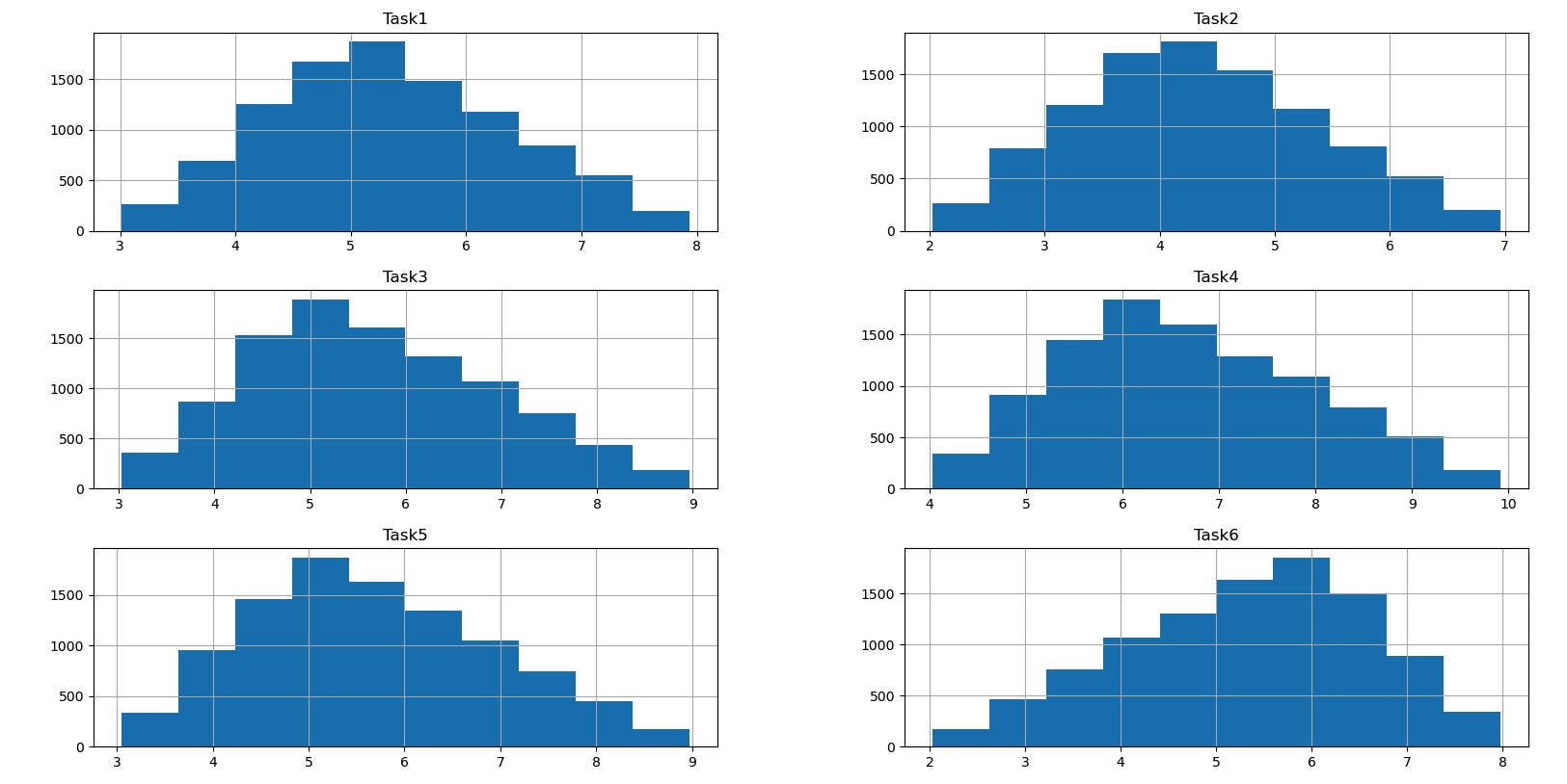
Figure 11.6 – Histograms of the values

By analyzing the previous diagram, we can confirm the triangular distribution of the time estimates, as we had imposed at the beginning of the calculations.

6. At this point, we only need to print the statistics of the total times. Let’s start with the minimum value:

   print(“Minimum project completion time = ",

                           np.amin(TotalTime))

The following result is returned:

Minimum project completion time =  14.966486785163458

Let’s analyze the average value:

print(“Mean project completion time = ",np.mean(TotalTime))

The following result is returned:

Mean project completion time =  23.503585938922157

Finally, we will print the maximum value:

print(“Maximum project completion time = ",np.amax(TotalTime))

The following result is printed:

Maximum project completion time =  31.90064194829465

In this way, we obtained an estimate of the time needed to complete the project based on Monte Carlo simulation.

Summary

In this chapter, we addressed several practical model simulation applications based on project management-related models. To start, we looked at the essential elements of project management and how these factors can be simulated to retrieve useful information.

Next, we tackled the problem of running a tiny forest for the wood trade. We treated the problem as a Markov decision process, summarizing the basic characteristics of these processes and then moved on to a practical discussion of them. We defined the elements of the problem and then we saw how to use the policy evaluation and policy improvement algorithms to obtain the optimal forest management policy. This problem was addressed using the MDPtoolbox package, which is available from Python.

Subsequently, we addressed how to evaluate the execution times of a project using Monte Carlo simulation. To start, we defined the task execution diagram by specifying which tasks must be performed in series and which can be performed in parallel. So, we introduced the times of each task through a three-point estimation. After this, we saw how to model the execution times of the project with triangular distribution using random evaluations of each phase. Finally, we performed 10,000 assessments of the overall project times.

In the next chapter, we will introduce the basic concepts of the fault diagnosis procedure. Then, we will learn how to implement a model for fault diagnosis for an induction motor. Finally, we will learn how to implement a fault diagnosis system for an unmanned aerial vehicle.