13

What’s Next?

In this chapter, we will summarize what has been covered so far in this book and what the next steps are. You will learn how to apply all the skills that you have gained to other projects, as well as the real-life challenges in building and deploying simulation models and other common technologies that data scientists use. By the end of this chapter, you will have a better understanding of the issues associated with building and deploying simulating models and will have broadened your knowledge of additional resources and technologies you can learn about to sharpen your machine learning skills.

In this chapter, we’re going to cover the following main topics:

• Summarizing simulation modeling concepts
• Applying simulation models to real life
• The next steps for simulation modeling

Summarizing simulation modeling concepts

Useful in cases where it is not possible to develop a mathematical model capable of effectively representing a phenomenon, simulation models imitate the operations performed over time by a real process. The simulation process involves generating an artificial history of the system to be analyzed; subsequently, the observation of this artificial history is used to trace information regarding the operating characteristics of the system itself and make decisions based on it.

The use of simulation models as a tool to aid decision-making processes has ancient roots and is widespread in various fields. Simulation models are used to study the behavior of a system over time and are built based on a set of assumptions made about the behavior of the system that’s expressed using mathematical-logical-symbolic relationships. These relationships are between the various entities that make up the system. The purpose of a model is to simulate changes in the system and predict the effects of these changes on the real system. For example, they can be used in the design phase before the model’s actual construction.

Important note

Simple models are resolved analytically, using mathematical methods. The solution consists of one or more parameters, called behavior measures. Complex models are simulated numerically on the computer, where the data is treated as being derived from a real system.

Let’s summarize the tools we have available to develop a simulation model.

Generating random numbers

In simulation models, the quality of the final application strictly depends on the possibility of generating good-quality random numbers. In several algorithms, decisions are made based on a randomly chosen value. The definition of random numbers suggests that of random processes through a connection that specifies its characteristics. A random number appears as such because we do not know how it was generated, but once the law within which it was generated is defined, we can reproduce it whenever we want.

Deterministic algorithms do not allow us to generate random number sequences, but simply make pseudo-random sequence generation possible. Pseudo-random sequences differ from random ones in that they are reproducible and, therefore, predictable.

Multiple algorithms are available for generating pseudorandom numbers. In Chapter 2, Understanding Randomness and Random Numbers, we analyzed the following in detail:

• Linear congruential generator (LCG): This generates a sequence of pseudo-randomized numbers using a piecewise discontinuous linear equation
• Lagged Fibonacci generator (LFG): This is based on a generalization of the Fibonacci sequence

More specific methods are added to these to generate uniform distributions of random numbers. The following graph shows a uniform distribution of 1,000 random numbers in the range of 1-10:

Figure 13.1 – A graph of the distribution of random numbers in the range of 1-10

We analyzed the following methods, both of which we can use to derive a generic distribution, starting from a uniform distribution of random numbers:

• Inverse transform sampling method: This method uses inverse cumulative distribution to generate random numbers.
• Acceptance-rejection method: This method uses the samples in the region under the graph of its density function.

A pseudo-random sequence returns integers uniformly distributed in each interval, with a very long repetition period and a low correlation level between one element of the sequence and the next.

To self-evaluate the skills that are acquired when generating random numbers, we can try to write some Python code for a bingo card generator. Here, we just limit the numbers from 1 to 90 and make sure that the numbers cannot be repeated and must be equally likely.

Applying Monte Carlo methods

A Monte Carlo simulation is a numerical method based on probabilistic procedures: Vine is widely used in statistics for the resolution of problems that present analytical difficulties that are not otherwise difficult to overcome. This method is based on the possibility of sampling an assigned probability distribution using random numbers. It generates a sequence of events distributed according to the assigned probability. In practice, instead of using a sample of numbers drawn at random, a sequence of numbers that has been obtained with a well-defined iterative process is used. These numbers are called pseudorandom because, although they’re not random, they have statistical properties such as those of true random numbers. Many simulation methods can be attributed to the Monte Carlo method, which aims to determine the typical parameters of complex random phenomena.

The following diagram describes the procedure leading from a set of distributions of random numbers to a Monte Carlo simulation:

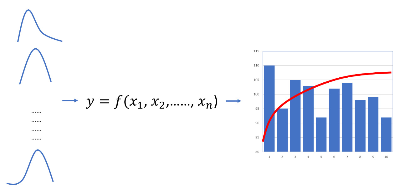
Figure 13.2 – The procedure of a Monte Carlo simulation, starting from a series of distributions of random numbers to one

The Monte Carlo method is essentially a numerical method for calculating the expected value of random variables, that is, an expected value that cannot be easily obtained through direct calculation. To obtain this result, the Monte Carlo method is based on two fundamental theorems of statistics:

• Law of large numbers: The simultaneous action of many random factors leads to a substantially deterministic effect.
• Central limit theorem: The sum of many independent random variables characterized by the same distribution is approximately normal, regardless of the starting distribution.

A Monte Carlo simulation is used to study the response of a model to randomly generated inputs.

Addressing the Markov decision process

Markov processes are discrete stochastic processes where the transition to the next state depends exclusively on the current state. For this reason, they can be called stochastic processes without memory. The typical elements of a Markovian process are the states in which the system finds itself and the available actions that the decision-maker can carry out in that state. These elements identify two sets: the set of states in which the system can be found, and the set of actions available for each specific state. The action chosen by the decision maker determines a random response from the system, which brings it into a new state. This transition returns a reward that the decision maker can use to evaluate their choice, as shown in the following diagram:

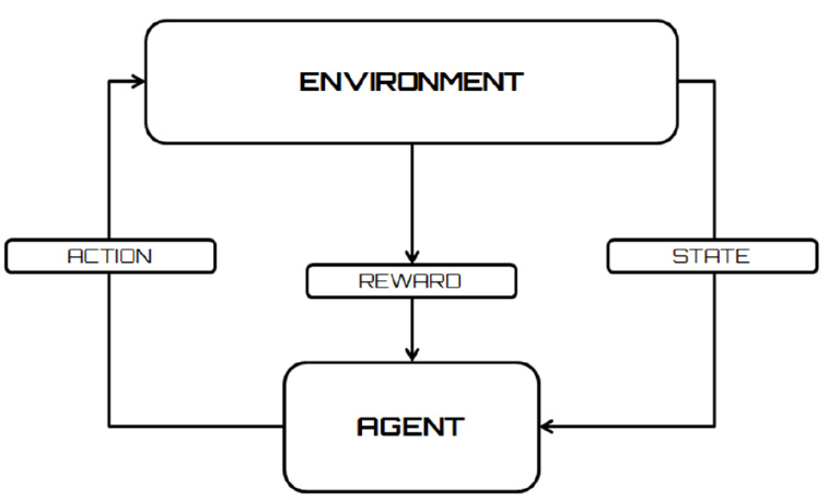
Figure 13.3 – A reward returned from the transition states

Crucial to the system’s future choices is the concept of reward, which represents the response of the environment to the action taken. This response is proportional to the weight that the action determines in achieving the objective – it will be positive if it leads to the correct behavior, while it will be negative in the case of a wrong action.

Another fundamental concept in Markovian processes is policy. A policy determines the system’s behavior in decision-making. It maps both the states of the environment and the actions to be chosen in those states, representing a set of rules or associations that respond to a stimulus. In a Markov decision-making model, the policy provides a solution that associates a recommended action with each state that can be achieved by the agent. If the policy provides the highest expected utility among the possible actions, it is called an optimal policy. In this way, the system does not have to keep its previous choices in memory. To make a decision, it only needs to execute the policy associated with the current state.

Now, let’s consider a practical application of a process that can be treated according to the Markov model. In a small industry, an operating machine works continuously. Occasionally, however, the quality of the products is no longer permissible due to the wear and tear of the spare parts, so the activity must be interrupted, and complex maintenance carried out. It is observed that the deterioration occurs after an operating time Tm of an average of 40 days, while maintenance requires a random time of an average of one day. How is it possible to describe this system with a Markovian model to calculate the probability at a steady state of finding the working machine?

The company cannot bear the downtime of the machine, so it keeps a second one ready to be used as soon as the first one requires maintenance. This second machine is, however, of lower quality, so it breaks after an exponential random work time of five days on average and requires an exponential time of one day on average to start again. As soon as the main machine is reactivated, the use of the secondary is stopped. If the secondary machine breaks before the main are reactivated, the repair team insists only on the main one being used, taking care of the second machine only after restarting the main. How is it possible to describe the system with a Markovian model, calculating the probability at a steady state with both machines stopped?

Think about how you might answer these questions using the knowledge you have gained from this book.

Analyzing resampling methods

In resampling methods, a subset of data is extracted randomly or according to a systematic procedure from an original dataset. The aim is to approximate the characteristics of a sample distribution by reducing the use of system resources.

Resampling methods are methods that repeat simple operations many times, generating random numbers to be assigned to random variables or random samples. These operations require more computational time as the number of repeated operations grows. They are very simple methods to implement and once implemented, they are automatic.

These methods generate dummy datasets from the initial data and evaluate the variability of a statistical property from its variability on all dummy datasets. The methods differ from each other in the way dummy datasets are generated. In the following diagram, you can see some datasets that were generated from an initial random distribution:

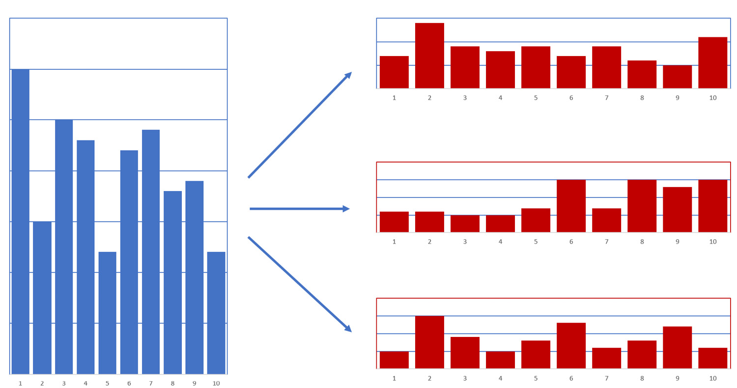
Figure 13.4 – Examples of datasets generated by an initial random distribution

There are many different resampling methods are available. In this book, we analyzed the following methods:

• Jackknife technique: Jackknife is based on calculating the statistics of interest for various sub-samples, leaving out one sample observation at a time. The jackknife estimate is consistent for various sample statistics, such as mean, variance, the relation coefficient, the maximum likelihood estimator, and others.
• Bootstrapping: The logic of the bootstrap method is to build samples that are not observed, but statistically like those observed. This is achieved by resampling the observed series through an extraction procedure where we reinsert the observations.
• Permutation test: Permutation tests are a special case of randomization tests and use a series of random numbers formulated from statistical inferences. The computing power of modern computers has made their widespread application possible. These methods do not require assumptions about data distribution to be met.
• Cross-validation technique: Cross-validation is a method used in model selection procedures based on the principle of predictive accuracy. A sample is divided into two subsets, of which the first (the training set) is used for construction and estimation and the second (the validation set) is used to verify the accuracy of the predictions of the estimated model.

Sampling is used if not all of the elements of the population are available. For example, investigations into the past can only be done on available historical data, which is often incomplete.

Exploring numerical optimization techniques

Numerous applications, which are widely used to solve practical problems, make use of optimization methods to drastically reduce the use of resources. Minimizing the cost or maximizing the profit of a choice are techniques that allow us to manage numerous decision-making processes. Mathematical optimization models are an example of optimization methods, in which simple equations and inequalities allow us to express the evaluation and avoid the constraints that characterize the alternative methods.

The goal of any simulation algorithm is to reduce the difference between the values predicted by the model and the actual values returned by the data. This is because a lower error between the actual and expected values indicates that the algorithm has done a good simulation job. Reducing this difference simply means minimizing an objective function that the model being built is based on.

In this book, we have addressed the following optimization methods:

• Gradient descent: This method is one of the first methods that was proposed for unconstrained minimization and is based on the use of the search direction in the opposite direction to that of the gradient, or anti-gradient. The interest of the direction opposite to the gradient lies precisely in the fact that, if the gradient is continuous then it constitutes a descent direction that is canceled if and only if the point that’s reached is a stationary point.
• Newton-Raphson: This method is used for solving numerical optimization problems. In this case, the method takes the form of Newton’s method for finding the zeros of a function but is applied to the derivative of the function f. This is because determining the minimum point of the function f is equivalent to determining the root of the first derivative.
• Stochastic gradient descent: This method solves the problem of evaluating the objective function by introducing an approximation of the gradient function. At each step, instead of the sum of the gradients being evaluated in correspondence with each data contained in the dataset, the evaluation of the gradient is used only in a random subset of the dataset.

Using artificial neural networks for simulation

Artificial neural networks (ANNs) are numerical models that have been developed with the aim of reproducing some simple neural activities of the human brain, such as object identification and voice recognition. The structure of an ANN is composed of nodes that, analogous to the neurons present in a human brain, are interconnected with each other through weighted connections, which reproduce the synapses between neurons. The system output is updated until it iteratively converges via the connection weights. The information that’s derived from experimental activities is used as input data and the result is processed by the network and returned as output. The input nodes represent the predictive variables that we need to process the dependent variables that represent the output neurons. The following diagram shows the functionality of an artificial neuron:

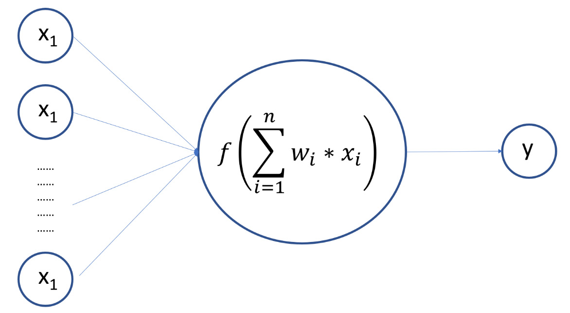
Figure 13.5 – The functionality of an artificial neuron

An ANN’s target is the result of calculating the outputs of all the neurons. This means an ANN is a set of mathematical function approximations. A model of this type can simulate the behavior of a real system, such as in pattern recognition. This is the process in which a pattern/signal is assigned to a class. A neural network recognizes patterns by following a training session, in which a set of training patterns are repeatedly presented to the network, with each category that they belong to specified. When a pattern that has never been seen before but belongs to the same category of patterns that it has learned is presented, the network will be able to classify it thanks to the information that was extracted from the training data. Each pattern represents a point in the multidimensional decision space. This space is divided into regions, each of which is associated with a class. The boundaries of these regions are determined by the network through the training process.

Now that we have recapped all the concepts we have learned about throughout this book, let’s see how they can be applied to challenges in the real world.

Applying simulation models to real life

The algorithms that we have analyzed in detail throughout this book represent valid tools for simulating real systems. Therefore, they are widely used in real life to carry out research on the possible evolution of a phenomenon, following a possible choice made on it.

Let’s look at some specific examples.

Modeling in healthcare

In the healthcare sector, simulation models have a significant weight and are widely used to simulate the behavior of a system to extract knowledge. For example, it is necessary to demonstrate the clinical efficacy of the health intervention under consideration before undertaking an economic analysis. The best available sources are randomized controlled trials. Trials, however, are often designed to leave out the economic aspects, so the key parameters for economic evaluations are generally absent. Therefore, a method is needed to evaluate the effect of disease progression, to limit the bias in the cost-effectiveness analysis. This implies the construction of a mathematical model that describes the natural history of the disease, the impact of the interventions applied on the natural history of the disease, and the results in terms of costs and objectives. The most used techniques are extrapolation, decision analysis, the Markov model, and Monte Carlo simulations:

• In extrapolation, the results of a trial with short follow-up periods are extrapolated beyond the end of the trial itself and various possible scenarios are considered, some more optimistic, in which the benefits associated with an intervention are assumed to be constant over time.
• The Markovian model is frequently used in pharmacoeconomic evaluations, especially following the numerous requests for cost-effectiveness evaluations by government organizations.
• An alternative to calculating the costs and benefits of a therapeutic option is Monte Carlo simulation. As in the Markov model, even in Monte Carlo simulation, precise states of health and the probability of transition are defined. In this case, however, based on the probability of transition and the result of a random number generator, a path is constructed for each patient until the patient themselves reaches the ultimate state of health envisaged by the model. This process is usually repeated for each patient in very large groups (even 10,000 cases), thus providing a distribution of survival times and related costs. The average values of costs and benefits obtained with this model are very similar to those that we would have calculated by applying the Markov model.
• However, Monte Carlo simulation also provides frequency distribution and variance estimates, which allow you to evaluate the level of uncertainty of the results of the model itself. In fact, Monte Carlo simulation is often used to obtain a sensitivity analysis of the results deriving from the application of the Markov model.

Modeling in financial applications

Monte Carlo simulation is normally used to predict the future value of various financial instruments. However, as highlighted previously, it is good to underline that this forecasting method is presented exclusively as an estimate and, therefore, does not provide a precise value as a result. The main financial applications of this method concern pricing options (or derivatives in general) and the evaluation of security portfolios and financial projects. From this, it is immediately evident that they present an element of analogy.

In fact, options, portfolios, and financial projects have a value that’s influenced by many sources of uncertainty. The simulation in question does not lend itself to the evaluation of any financial instrument. Securities such as shares and bonds are not normally valued with the method, precisely because their value is subordinated to a lower number of sources of uncertainty.

The options, on the contrary, are derivative securities, the value of which is influenced by the performance of the underlying functions (which may have the most varied content) and by numerous other factors (interest rates, exchange rates, and so on). Monte Carlo simulation allows you to generate pseudorandom values for each of these variables and assign a value to the desired option. It should be noted, however, that the Monte Carlo method is only one of the pricing options available.

Continuing with the category of financial instruments, portfolios are sets of different securities, normally of a varied nature. Portfolios are exposed to a variety of sources of risk. The operational needs of modern financial intermediaries have led to the emergence of calculation methods that aim to monitor the overall risk exposure of their portfolios. The main method in this context is VaR (value at risk), which is often calculated using Monte Carlo simulation.

Ultimately, when a company must evaluate the profitability of a project, it will have to compare the cost of the same with the revenue generated. The initial cost is normally (but not necessarily) certain. The cash flows that are generated, however, are hardly known a priori. The Monte Carlo method allows us to evaluate the profitability of the project by attributing pseudorandom values to the various cash flows.

Modeling physical phenomenon

The simulation of a physical model allows you to experiment with the model by putting it to the test by changing its parameters. The simulation of a model, therefore, allows you to experiment with the various possibilities of the model, as well as its limits, in terms of how the model acts as a framework for the experimentation and organization of our ideas. When the model works, it is possible to remove the scaffolding. In this situation, maybe it turns out that it stands up or something new has been discovered. When constructing a model, reference is made to the ideas and knowledge through which the reality of the phenomenon is formally represented.

Just as there is no univocal way to face and solve problems, there is no univocal way to construct the models that describe the behavior of a given phenomenon. The mathematical description of reality struggles to keep considerations of the infinite, complex, and related aspects that represent a physical phenomenon. If the difficulty is already significant for a physical phenomenon, it will be even greater in the case of a biological phenomenon.

The need to select between relevant and non-relevant variables leads to discrimination between these variables. This choice is made thanks to ideas, knowledge, and the school that those who work on the model come from.

Random phenomena permeate everyday life and characterize various scientific fields, including mathematics and physics. The interpretation of these phenomena experienced a renaissance in the middle of the last century with the formulation of Monte Carlo methods. This milestone was achieved thanks to the intersection of research on the behavior of neurons in a chain reaction and the results achieved in the electronic field with the creation of the first computer. Today, simulation methods based on random number generation are widely used in physics.

One of the key points of quantum mechanics is to determine the energy spectrum of a system. This problem, albeit with some complications, can be resolved analytically in the case of very simple systems. In most cases, however, an analytical solution does not exist. Because of this, there’s a need to develop and implement numerical methods capable of solving the differential equations that describe quantum systems. In recent decades, due to technological development and the enormous growth in computing power, we have been able to describe a wide range of phenomena with incredibly high precision.

Modeling fault diagnosis system

To meet the needs of industrial processes in the continuous search for ever higher performance, the control systems are gradually becoming more complex and sophisticated. Consequently, it is necessary to use special supervision, monitoring, and diagnosis devices within the control chain of malfunctions capable of guaranteeing the efficiency, reliability, and safety of the process in question.

Most industrial processes involve the use of diagnostic systems with a high degree of reliability. Examples of types of diagnostic systems are as follows:

• Diagnostic systems based on hardware redundancy: These are based on the use of additional/redundant hardware to replicate the signals of the components being monitored. The diagnosis mechanism provides for the analysis of the output signals to the redundant devices. If one of the signals deviates significantly from the others when following this analysis, then the component is classified as malfunctioning.
• Diagnostic systems based on probability analysis: This method is based on verifying the likelihood between the output signal generated by a component and the physical law that regulates its operation.
• Diagnostic systems based on the analysis of signals: This methodology assumes that when starting from the analysis of certain output signals of a process, it is possible to obtain information regarding any malfunctions.
• Systems based on machine learning: These methods provide for the identification and selection of functions and the classification of faults, allowing a systematic approach to fault diagnosis. They can be used in automated and unattended environments.

Modeling public transportation

In recent years, the analysis of issues related to vehicular traffic has taken on an increasingly important role in trying to develop well-functioning transport within cities and on roads in general. Today’s transport systems need an optimization process that is coordinated with a development that offers concrete solutions to requests. Through better transportation planning, a process that produces fewer cars in the city and more parking opportunities should lead to a decrease in congestion.

A heavily slowed and congested urban flow can not only inconvenience motorists due to the increase in average travel, but can also make road circulation less safe and increase atmospheric and noise pollution.

Many causes have led to an increase in traffic, but certainly the most important is the strong increase in overall transport demand; this increase is due to factors of a different nature, such as a large diffusion of cars, a decentralization of industrial and city areas, and an often-lacking public transport service.

To try and solve the problem of urban mobility, we need to act with careful infrastructure management and with a traffic network planning program. An important planning tool could be a model of the traffic system, which essentially allows us to evaluate the effects that can be induced on it by interventions in the transport networks, while also allowing us to compare different design solutions. The use of a simulation tool allows us to evaluate some decisional or behavioral problems, quickly and economically, where it is not possible to carry out experiments on the real system. These simulation models represent a valid tool available to technicians and decision-makers in the transport sector for evaluating the effects of alternative design choices. These models allow for a detailed analysis of the solutions being planned at the local level.

There are simulation tools available that allow us to represent traffic accurately and specifically and map its evolution instant by instant, all while taking the geometric aspects of the infrastructure and the real behavior of the drivers into consideration, both of which are linked to the characteristics of the vehicle and the driver. Simulation models allow these to be represented on a small scale and, therefore, at a relatively low cost, as well as the effects and consequences related to the development of a new project. Micro-simulations provide a dynamic vision of the phenomenon since the characteristics of the motion of the individual vehicles (flow, density, and speed) are no longer considered, but real and variable, instant by instant during the simulation.

Modeling human behavior

The study of human behavior in the case of a fire, or cases of a general emergency, presents difficulties that cannot be easily overcome since many of the situations whose data it would be important to know about cannot be simulated in laboratory settings. Furthermore, the reliability of the data drawn from exercises in which there are no surprises or anxiety effects such as stress, as well as the possibility of panic that can occur in real situations, can be considered relative. Above all, the complexity of human behavior makes it difficult to predict the data that would be useful for fire safety purposes.

Studies conducted by scientists have shown that the behaviors of people during situations of danger and emergency are very different. In fact, research has shown that during an evacuation, people will often do things that are not related to escaping from the fire, and these things can constitute up to two-thirds of the time it takes an individual to leave the building. People often want to know what’s happening before evacuating, as the alarm does not necessarily convey much information about the situation.

Having a simulation model capable of reproducing a dangerous situation is extremely useful for analyzing the reactions of people in such situations. In general terms, models that simulate evacuations address this problem in three different ways: optimization, simulation, and risk assessment.

The underlying principles of each of these approaches influence the characteristics of each model. Numerous models assume that occupants evacuate the building as efficiently as possible, ignoring secondary activities and those not strictly related to evacuation. The escape routes chosen during the evacuation are considered optimal, as are the characteristics of the flow of people toward the exits. The models that consider many people and that treat the occupants as a homogeneous whole, therefore without giving weight to the specific behavior of the individual, tend toward these aspects.

Next steps for simulation modeling

For most of human history, it has been reasonable to expect that when you die, the world will not be significantly different from when you were born. Over the past 300 years, this assumption has become increasingly outdated. This is because technological progress is continuously accelerating. Technological evolution translates into a next-generation product better than the previous one. This product is therefore a more efficient and effective way of developing the next stage of evolutionary progress. It is a positive feedback circuit. In other words, we are using more powerful and faster tools to design and build more powerful and faster tools. Consequently, the rate of progress of an evolutionary process increases exponentially over time, and the benefits such as speed, economy, and overall power also increase exponentially over time. As an evolutionary process becomes more effective and/or efficient, more resources are then used to encourage the progress of this process. This translates into the second level of exponential growth; that is, the exponential growth rate itself grows exponentially.

This technological evolution also affects the field of numerical simulation, which must be compared with the users’ need to have more performant and simpler to make models. The development of a simulation model requires significant skills in model building, experimentation, and analysis. If we want to progress, we need to make significant improvements in the model-building process to meet the demands that come from the decision-making environment.

Increasing the computational power

Numerical simulation is performed by computers, so higher computational powers make the simulation process more effective. The evolution of computational power was governed by Moore’s law, named after the Intel founder who predicted one of the most important laws regarding the evolution of computational power: every 18 months, the power generated by a chip doubles in computing capacity and halves in price.

When it comes to numerical simulation, computing power is everything. Today’s hardware architectures are not so different from those of a few years ago. The only thing that has changed is the power of processing information. In the numerical simulation, information is processed: the more complex a situation becomes, the more the variables involved increase.

The growing processing capacity required for software execution and the increase in the amount of input data has always been satisfied by the evolution of central processing units (CPUs), according to Moore’s law. However, lately, the growth of the computational capacity of CPUs has slowed down and the development of programming platforms has posed new performance requirements that create a strong discontinuity with respect to the hegemony of these CPUs with new hardware architectures in strong diffusion both on the server and on the device’s side. In addition, the growing distribution of intelligent applications requires the development of specific architectures and hardware components for the various computing platforms.

Graphical processing units (GPUs) were created to perform heavy and complex calculations. They consist of a parallel architecture made up of thousands of small and efficient cores, designed for the simultaneous management of multiple operations.

Field programming gateway array (FPGA) architectures are integrated circuits designed to be configured after production based on specific customer requirements. FPGAs contain a series of programmable logic blocks and a hierarchy of reconfigurable interconnections that allow the blocks to be “wired together.”

The advancement of hardware affects not only computing power but also storage capacity. We cannot send information at 1 GBps without having a physical place to contain it. We cannot train a simulation architecture without storing a dataset of several terabytes in size. Innovating means seeing opportunities that were not there previously by making use of components that constantly become more efficient. To innovate means to see what can be done by combining a more performant version of the three accelerators.

Machine-learning-based models

Machine learning is a field of computer science that allows computers to learn to perform a task without having to be explicitly programmed for its execution. Evolved from the studies on pattern recognition and theoretical computational learning in the field of artificial intelligence, machine learning explores the study and construction of algorithms that allow computers to learn information from available data and predict new information in light of what has been learned. These algorithms overcome the classic paradigm of strictly static instructions by building a model that automatically learns to predict new data from observations, finding its main use in computing problems where the design and implementation of ad hoc algorithms are not practicable or convenient.

Machine learning has deep links to the field of numerical simulation, which provides methods, theories, and domains of application. In fact, many machine learning problems are formulated as problems regarding minimizing a certain loss function against a specific set of examples (the training set). This function expresses the discrepancy between the values predicted by the model during training and the expected values for each example instance. The goal is to develop a model capable of correctly predicting the expected values in a set of instances never seen before, thus minimizing the loss function. This leads to a greater generalization of prediction skills.

The different machine learning tasks are typically classified into three broad categories, characterized by the type of feedback that the learning system is based on:

• Supervised learning: The sample inputs and the desired outputs are presented to the computer, with the aim of learning a general rule capable of mapping the inputs to the outputs.
• Unsupervised learning: The computer only provides input data, without any expected output, with the aim of learning some structure in the input data. Unsupervised learning can represent a goal or aim to extrapolate salient features of the data that are useful for executing another machine learning task.
• Reinforcement learning: The computer interacts with a dynamic environment in which it must achieve a certain goal. As the computer explores the domain of the problem, it is given feedback in terms of rewards or punishments in order to direct it toward the best solution.

The following diagram shows the different types of machine learning algorithms:

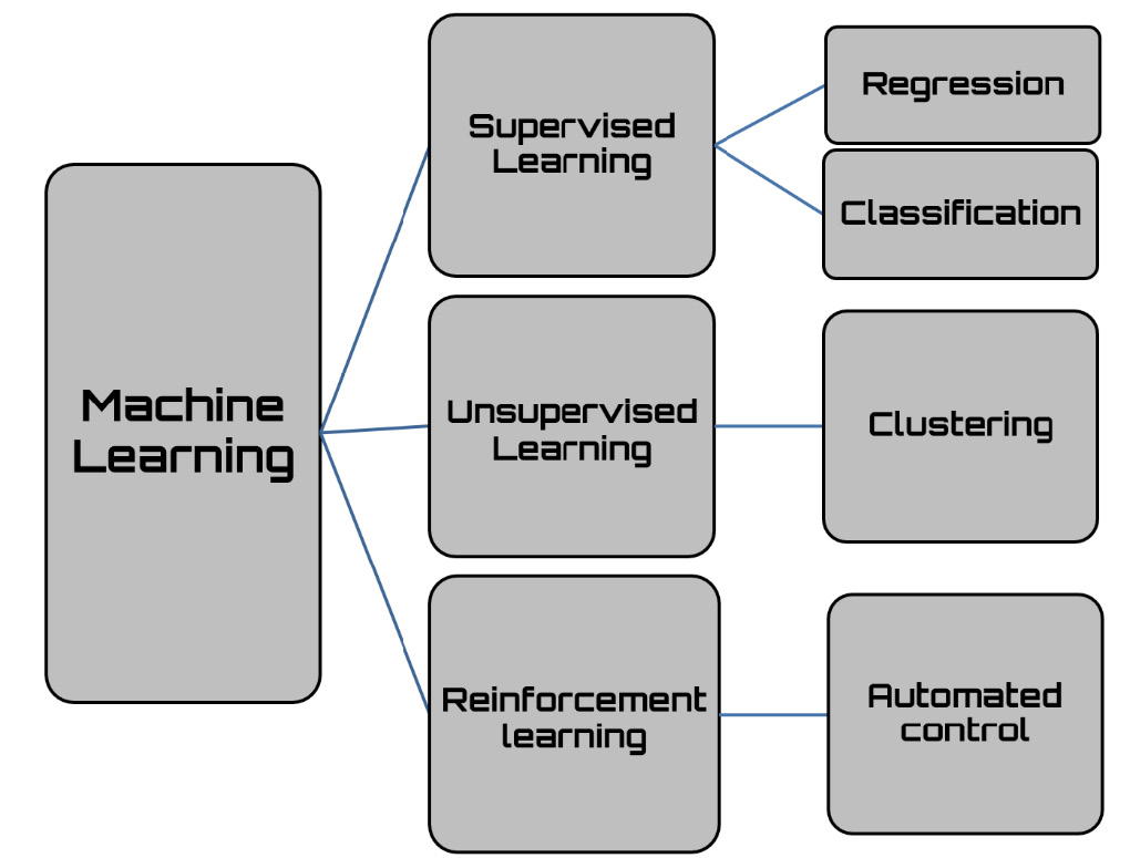
Figure 13.6 – The different types of machine learning algorithms

Automated generation of simulation models

Automated machine learning (AutoML) defines applications that can automate the end-to-end process of applying machine learning. Usually, technical experts must process data through a series of preliminary procedures before submitting it to machine learning algorithms. The steps necessary to perform a correct analysis of the data through these algorithms require specific skills that not everyone has. Although it is easy to create a model based on deep neural networks using different libraries, knowledge of the dynamics of these algorithms is required. In some cases, these skills are beyond those possessed by analysts, who must seek the support of industry experts to solve the problem.

AutoML has been developed to create an application that automates the entire machine learning process so that the user can take advantage of these services. Typically, machine learning experts should perform the following activities:

• Preparing the data
• Selecting features
• Selecting an appropriate model class
• Choosing and optimizing model hyperparameters
• Post-processing machine learning models
• Analyzing the results obtained

AutoML automates all these operations. It offers the advantage of producing simpler and faster-to-create solutions that often outperform hand-designed models. There are several AutoML frameworks available, each of which has characteristics that indicate its preferential use.

Summary

In this chapter, we summarized the technologies that we have exposed throughout this book. We have seen how to generate random numbers and have listed the most frequently used algorithms used to generate pseudo-random numbers. Then, we saw how to apply the Monte Carlo methods for numerical simulation based on the assumptions of two fundamental laws: the law of large numbers and the central limit theorem. We then went on to summarize the concepts that Markovian models are based on and then analyzed the various available resampling methods. After that, we explored the most used numerical optimization techniques and learned how to use artificial neural networks for numerical simulation.

Subsequently, we mentioned a series of fields in which numerical simulation is widely used and then looked at the next steps that will allow simulation models to evolve.

In this book, we studied various computational statistical simulations using Python. We started with the basics to understand various methods and techniques to deepen our knowledge of complex topics. At this point, the developers working with a simulation model would be able to put their knowledge to work, adopting a practical approach to the required implementation and associated methodologies so that they’re operational and productive in no time. I hope that I have provided detailed explanations of some essential concepts using practical examples and self-assessment questions, exploring numerical simulation algorithms, and providing an overview of the relevant applications to help you make the best models for your needs.