Chapter 8: Introduction to Python
In this chapter, we will be learning about the Python commands and functionalities while applying them to problems. As we delve into the first chapter of Section 2, Applying Python and Computational Thinking, we will be using more complex Python programming. In this chapter, we will focus more on language, while the remaining chapters will focus on application.
In this chapter, we will cover the following topics:
- Introducing Python
- Working with dictionaries and lists
- Using variables and functions
- Learning about files, data, and iteration
- Using object-oriented programming
As we dig deeper into the Python programming language, remember that some of the content has been covered in previous chapters as we looked at the computational thinking process, such as the use of dictionaries and functions. This chapter will allow you to find critical information more easily when looking for Python commands to meet your computational thinking problem needs.
Technical requirements
You will need the latest version of Python to run the codes in this chapter. You will find the full source code used in this chapter here: https://github.com/PacktPublishing/Applied-Computational-Thinking-with-Python/tree/master/Chapter08
Introducing Python
Python is one of the fastest-growing programming languages due to its ease of use. One of the draws of Python is that we can write the same programs we do with languages such as C, C++, and Java, but with fewer lines of code and simpler language and syntax. Another big draw of Python is that it is extensible, which means we can add capabilities and functionalities to it.
While not all functionalities are inherently built in, we can use libraries to add what we need. Those libraries are available to download and use. For example, if we wanted to work with data and data science, there are a few libraries we can download, such as Pandas, NumPy, Matplotlib, SciPy, Scikit Learn, and more. But before we get into those libraries, let's look at how the Python language works and learn its basics.
Python has some built-in reference functions. The following table shows the functions in alphabetical order:
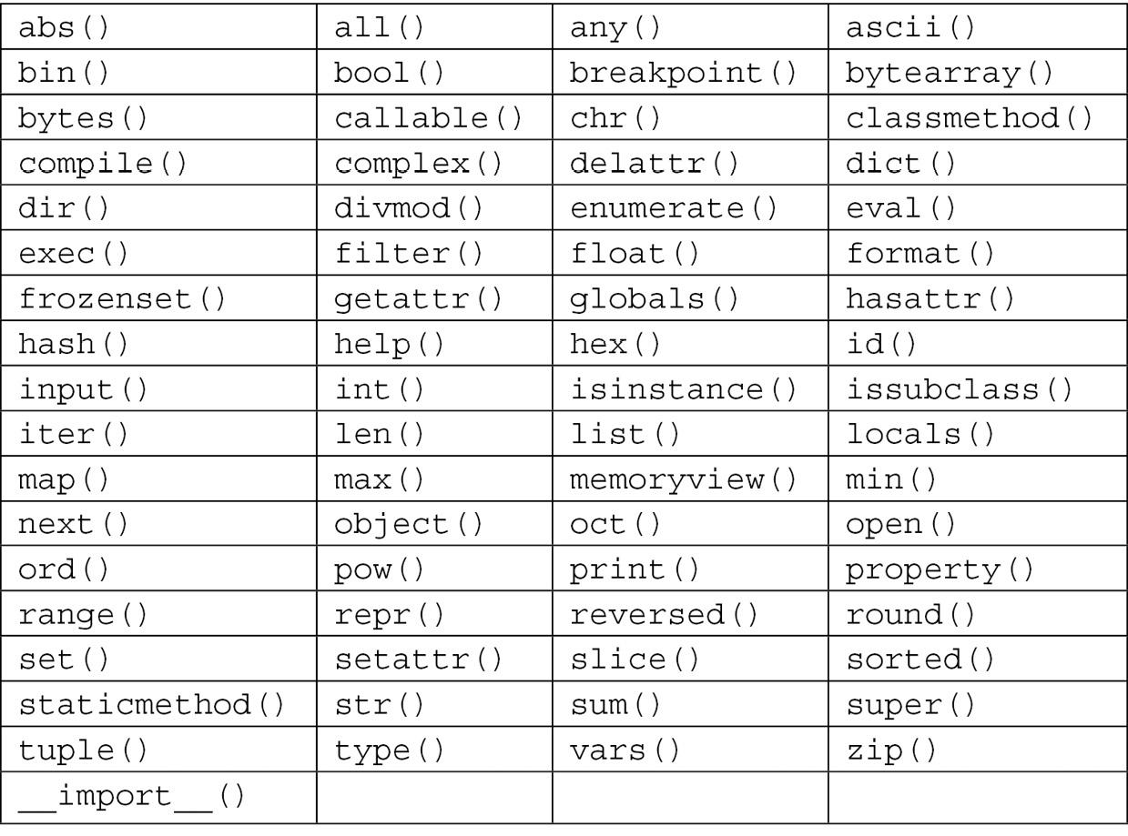
Table 8.1 – Python built-in functions
While we won't go over all the functions in this book, we will use some of them as we look at Python and its algorithms. Let's start with some of the mathematical functions listed here.
Mathematical built-in functions
In Python, some of the mathematical functions are already built in, such as the abs(), eval(), max(), min(), and sum() functions. These are not the only mathematical functions built in, but we'll take a closer look at these particular ones in order to understand how Python deals with them.
The abs() function will help us find the absolute value of a number, either an integer or a float. Take a look at the following code snippet:
ch8_absFunction.py
x = abs(-3.89)
print(x)
When we run this program, we'll get the absolute value of –3.89. Remember that the absolute value of a number is its distance from 0. Take a look at the output when we run this program:
3.89
Since the absolute value is always positive, when we run abs(–3.89), we get 3.89.
Another helpful mathematical function is the eval() function. We can define a variable in this function and then call for Python to evaluate an algebraic expression using that value. In the Python shell, we can first define the variable as follows:
>>> p = 2
Now that the variable is defined, we can call the eval() function with any expression. For example, take a look at the following input and output:
>>> eval('2 * p - 1')
As you can see, Python used the previously defined p value of 2, and substituted then evaluated the expression to produce this output:
3
The Python program also works as a calculator, so you can perform mathematical operations as you normally would. Here are a few examples:
>>> 10-8
As you can see, Python knows to read the dash as a subtraction and produces the result of the mathematical expression:
2
In the next case, Python interpreted + as a mathematical symbol and provided the result of the sum expression:
>>> 4+5
The output is:
9
Notice the last expression, 10**5. In Python, we can use two stars (**) to denote exponents:
>>> 10**5
The output is:
100000
Now, let's take a look at the max() function. This function can be used on an iterable list, but we can test it with just two numbers:
>>> max(12, 30)
You can clearly see what the output is:
30
Let's take another example:
>>> max(100, 10)
This is the output:
100
As you can see from the output, the function always chooses the largest item. You can add a third item and the function will still choose the maximum value. These built-in functions are smart in a way that they are coded to work with what is provided – two or three items, for example – without having to tell Python explicitly how many items we'll be introducing:
>>> max(230, 812, 109)
The output obtained is:
812
As you can see, we did not have to add anything to the built-in function to find the maximum of three values.
The min() function is the opposite; it chooses the minimum value. Take a look at the following minimum function:
>>> min(230, 812, 109)
This is the output:
109
As you can see, the function used the same list we used for the maximum function, but this time the output is 109, which is the minimum value of that group of numbers.
There are other mathematical functions, such as sum(). If you're a Python beginner, it's recommended that you play around with those functions to learn how they work. These functions will be key to your algorithms as you design solutions for computational thinking problems. We will also use some of these functions as we look at other Python functionalities, such as dictionaries and arrays.
Working with dictionaries and lists
Before we get too deep into dictionaries and lists, it's important to note that Python does not contain arrays in the built-in functions. We can use lists and perform a lot of the traditional functions on lists that we'd use for arrays. However, for more robust functionalities with arrays, a library is needed, such as NumPy.
Python has four collection data types, which are as follows:
- Lists: Ordered and changeable; can have duplicates
- Tuples: Ordered and unchangeable; can have duplicates
- Sets: Unordered and unindexed; cannot have duplicates
- Dictionaries: Unordered, changeable, and indexed; cannot have duplicates
As noted, we won't be going into NumPy libraries or other data libraries just yet. For now, we're going to focus on dictionaries and lists.
Defining and using dictionaries
You may recall that we used dictionaries in Chapter 3, Understanding Algorithms and Algorithmic Thinking, when we created a menu of items. Dictionaries in Python are collections that have the following three characteristics:
- They are unordered.
- They are changeable.
- They are indexed by keys.
Dictionaries are organized as value pairs. For example, we can have a dictionary with value pairs of states and their capitals. Take a look at the following dictionary:
ch8_dictionary1.py
states = {
'Ohio':'Columbus',
'Delaware':'Dover',
'Pennsylvania':'Harrisburg',
'Vermont':'Montpelier'
}
print(states)
If we were to print this dictionary without any conditions to the print statement, we would get the following output:
{'Ohio': 'Columbus', 'Delaware': 'Dover', 'Pennsylvania': 'Harrisburg', 'Vermont': 'Montpelier'}
As you can see, each value pair is printed at once. Just like we built the dictionary in this way, Python also has a built-in dict() function. The same dictionary can be built using that function, as follows:
ch8_dictionary2.py
states = dict([
('Ohio','Columbus'),
('Delaware','Dover'),
('Pennsylvania','Harrisburg'),
('Vermont','Montpelier')
])
print(states)
You can see that the dictionary is constructed very similarly in both examples, with some changes in syntax, such as the use of colons in the first instance, versus parentheses and commas in the second one. However, the print statement produces the same result.
Dictionaries are said to be key-value pairs because the first item is the key and the second, paired item is the value. So, for Ohio and Columbus, Ohio is the key while Columbus is the value. We can use the key to call any value. For example, I can call states['Ohio'] and it should return 'Columbus'. Take a look at the code:
>>> states['Ohio']
This is the output:
'Columbus'
We can do that for any key-value pair in the dictionary. But if we try to call a key that's not in the dictionary, such as Alabama, then we get the following error:
>>> states['Alabama']
This leads to the following error being displayed:
Traceback (most recent call last):
File "<pyshell#23>", line 1, in <module>
states['Alabama']
KeyError: 'Alabama'
Notice that this gives a KeyError, mentioned in the list of errors in Chapter 7, Identifying Challenges within Solutions, in the Errors in logic section. But let's say we do want to add Alabama and the capital, which is Montgomery. We can use the following code to do so:
>>> states['Alabama'] = 'Montgomery'
We can call the dictionary again after entering the following code:
>>> print(states)
This gives us the following output:
{'Ohio': 'Columbus', 'Delaware': 'Dover', 'Pennsylvania': 'Harrisburg', 'Vermont': 'Montpelier', 'Alabama': 'Montgomery'}
Notice that the dictionary added the 'Alabama':'Montgomery' key-value pair at the end of the dictionary.
We can also delete key-value pairs using the del code, as shown:
>>> del states['Delaware']
Now, if we go ahead and print the states dictionary, Delaware is no longer on the list:
>>> print(states)
This is the output after deleting the state:
{'Ohio': 'Columbus', 'Pennsylvania': 'Harrisburg', 'Vermont': 'Montpelier', 'Alabama': 'Montgomery'}
Now, you can continue to add items or delete them without having to go into the main algorithm.
With dictionaries, you can also add multiple values to one key. Let's say I play three sports (I don't). I could list those in a dictionary and match them to one key value. Take a look at the following algorithm:
ch8_dictionary3.py
miscellaneous = {
'sports' : ['tennis', 'bowling', 'golf'],
'age' : '40',
'home' : 'lake'
}
We can print the full dictionary using print(miscellaneous), as follows:
>>> print(miscellaneous)
This is how we get the output:
{'sports': ['tennis', 'bowling', 'golf'], 'age': '40', 'home': 'lake'}
As you can see, the printed dictionary includes all the values. If I want to print only the sports, then I can use the miscellaneous['sports'] code:
>>> miscellaneous['sports']
This is the output:
['tennis', 'bowling', 'golf']
Notice that we did not use the print() function at all. We used the dictionary, which we called miscellaneous, and called the 'sports' key. Note that we were able to get this result because we called the dictionary in the IDLE command window in Python. If you want to include this in your algorithm, you'll still need to use the print() function.
While we won't go into all the functionalities of dictionaries here, you can see how they can be helpful in creating algorithms that contain key-value pairs. Python allows us to add and alter the dictionary, call values, and more with the use of simple code without having to access the entire dictionary to do so.
Next, we'll take a look at lists.
Defining and using lists
Lists in Python are ordered and changeable. We can create lists for anything, such as types of animals, colors, fruit, numbers, or really whatever we want. Since we can have duplicate values, we could have a list for three apples that just says apple, apple, apple. For example, take a look at the list shown:
ch8_list1.py
fruits = ['apple','apple','apple']
print(fruits)
When we print this list, all the items are included. The output is as follows:
['apple', 'apple', 'apple']
As you can see, we have the same value three times. We would not be able to do that with a dictionary, which does not allow duplicate members.
Now, let's take a look at what we can do with lists. Let's start with the following list of animals:
ch8_list2.py
animals = ['dog', 'cat', 'bird', 'lion', 'tiger', 'elephant']
The first item in the list is 'dog'. Lists have indexes, starting at 0. So, if we printed animals[0], we'd get dog. We can check it here:
>>> print(animals[0])
This is the output with index 0:
dog
There are six items on the list, but the last index is [5]. So, to print elephant, we'd need to print using that index:
>>> print(animals[5])
elephant
You can also use negative numbers for indexes in lists. The [–1] index refers to the last index, so it represents elephant, the same as index [5]:
>>> print(animals[-1])
elephant
The [–2] index refers to the second-to-last index, so tiger, and so on.
We can also print multiple items from a list by specifying a range of indexes. Take a look at the following code:
>>> print(animals[1:4])
This is the output:
['cat', 'bird', 'lion']
As you can see, we printed the second item on the list, which corresponds to index [1], and the next two items.
With lists, we can also add items, replace items, delete items, check for the length, and more. To add an item, we need to use the append() method. Let's add the duck item to our list:
>>> animals.append('duck')
>>> print(animals)
Here is the added item:
['dog', 'cat', 'bird', 'lion', 'tiger', 'elephant', 'duck']
Notice that our list now has duck at the end of the list. But let's say we want to remove bird and substitute it with butterfly:
First, we have to identify the index for bird. That index is 2, as it is the third item on the list:
>>> animals[2] = 'butterfly'
>>> print(animals)
Here is the output, with bird replaced:
['dog', 'cat', 'butterfly', 'lion', 'tiger', 'elephant', 'duck']
The list now contains butterfly.
Removing an item is fairly straightforward, as we just use the remove() method and the item we want to remove:
>>> animals.remove('lion')
>>> print(animals)
As you can see, lion has been removed from the list:
['dog', 'cat', 'butterfly', 'tiger', 'elephant', 'duck']
We can also remove an item by index using the pop() method. Using index 1 removes the second item on the list. Refer to the following code:
>>> animals.pop(1)
'cat'
Then, we can try the following:
>>> print(animals)
['dog', 'butterfly', 'tiger', 'elephant', 'duck']
Notice that Python identifies the item at index 1 that was popped out of the list. When we print the list again, the item is no longer there. If we want to remove the last item, we do not have to specify an index. Refer to the following code:
>>> animals.pop()
'duck'
Then, we can try the following:
>>> print(animals)
['dog', 'butterfly', 'tiger', 'elephant']
As mentioned, when no index is specified, the last item on the list is popped and removed from the list.
There is yet another way to remove an item from the list, by using the del keyword:
>>> del animals[1]
>>> print(animals)
This is the output:
['dog', 'tiger', 'elephant']
Our list lost the second item on the list. We can also use the del keyword to delete the list entirely:
>>> del animals
>>> print(animals)
This error is the output here:
Traceback (most recent call last):
File "<pyshell#49>", line 1, in <module>
print(animals)
NameError: name 'animals' is not defined
As you can see, I can no longer print the list because it is not defined. Notice we received a NameError description of name 'animals' is not defined. This is one of the other errors mentioned in Chapter 7, Identifying Challenges within Solutions.
Important Note:
For the next few code examples, I ran my original code from the ch8_list2.py file again to get my original list.
We can clear an entire list without eliminating the actual list by using the clear() method, as follows.
>>> animals.clear()
>>> print(animals)
This is the output we get:
[]
In this case, the list now prints as an empty list without giving an error message. That's because the list is still there and defined, it's just empty.
Now, let's say I wanted the length of my list. We can find the length of the list by using len(). Again, I went back to the original list to run the following code:
>>> print(len(animals))
We get the following output:
6
Our original list contained six elements – that is, six animals.
Now, let's define another list that contains colors:
ch8_list3.py
animals = ['dog', 'cat', 'bird', 'lion', 'tiger', 'elephant']
colors = ['blue', 'red', 'yellow']
print(animals)
print(colors)
The output for this algorithm is two lists. Now, if we wanted to combine the two lists, we could do so using the extend() method.
Let's take a look at how we can append colors to the animals list:
>>> animals.extend(colors)
>>> print(animals)
This is the appended list:
['dog', 'cat', 'bird', 'lion', 'tiger', 'elephant', 'blue', 'red', 'yellow']
Our list now includes all our animals and all our colors. We could have also used the following method to extend colors with animals. The difference is that the colors would appear first on our list:
>>> colors.extend(animals)
>>> print(colors)
This is how the list now appears:
['blue', 'red', 'yellow', 'dog', 'cat', 'bird', 'lion', 'tiger', 'elephant']
We can also sort lists, which is helpful when we want to have an alphabetical list or if we want to sort a list of numbers. Take a look at the two lists in the following algorithm:
ch8_list4.py
animals = ['dog', 'cat', 'bird', 'lion', 'tiger', 'elephant']
numbers = [4, 1, 5, 8, 2, 4]
print(animals)
print(numbers)
This is how they appear unsorted:
['dog', 'cat', 'bird', 'lion', 'tiger', 'elephant']
[4, 1, 5, 8, 2, 4]
Let's sort both lists and see what happens:
>>> numbers.sort()
>>> print(numbers)
We will get this output:
[1, 2, 4, 4, 5, 8]
Then, we can try the following:
>>> animals.sort()
>>> print(animals)
We get this as the output:
['bird', 'cat', 'dog', 'elephant', 'lion', 'tiger']
As you can see, the numbers were sorted from smallest to largest, while the animals were sorted in alphabetical order.
Let's talk for a second about why this is so helpful. Imagine that you have a list of items displayed on your website that come from a Python list. They are all sorted and perfectly displayed. But let's now say you want to add more items. It's easier to add them in any order to your list using the methods we have discussed, then we can sort them so that they continue to be in alphabetical order.
Of course, these are not the only things we can do with lists. Python allows us to work with lists in many ways that are user-friendly and function similar to what arrays do in other programming languages. When we need to use them in other ways, we can search for libraries that contain those functionalities.
Both lists and dictionaries are important in the Python programming language. In this section, you saw that dictionaries use key-value pairs, while lists include values. Both can be edited using methods and functions built into the Python programming language. You'll see them again when we apply Python to more complex computational thinking problems in Section 3, Data Processing, Analysis, and Applications Using Computational Thinking and Python, of this book.
Now, we'll take a look at how we use variables and functions in Python.
Using variables and functions
In Python, we use variables to store a value. We can then use the value to perform operations, evaluate expressions, or use them in functions. Functions give sets of instructions for the algorithm to follow when they are called in an algorithm. Many functions include variables within them. So, let's first look at how we define and use variables, then take a look at Python functions.
Variables in Python
Python does not have a command for declaring variables. We can create variables by naming them and setting them equal to whatever value we'd like. Let's take a look at an algorithm that contains multiple variables:
ch8_variables.py
name = 'Marcus'
b = 10
country_1 = 'Greece'
print(name)
print(b)
print(country_1)
As you can see, we can use a letter, a longer name, and even include underscores in naming our variables. We cannot, however, start a variable name with a number. When we run this program, we get the following output:
Marcus
10
Greece
Each variable was printed without any problems. If we had used a number to begin any variable name, we would have gotten an error. However, if I had named the country_1 variable as _country, that would be an acceptable variable name in Python.
Now, let's take a look at what we can do with variables.
Combining variables
One thing variables allow us to do is combine them in a print statement. For example, I can create a print statement that prints Marcus Greece. To do so, I can use the + character, as follows:
>>> print(name + ' ' + country_1)
Notice that between the two + characters, there's ' '. This is done to add a space so that our print statement won't look like MarcusGreece. Now, let's combine b and name in a print statement:
>>> print(b + name)
This will give us an error message:
Traceback (most recent call last):
File "<pyshell#70>", line 1, in <module>
print(b + name)
TypeError: unsupported operand type(s) for +: 'int' and 'str'
Notice that the error states TypeError: unsupported operand types for +. It also states that we have 'int' and 'str', which means we are combining two different data types.
To be able to combine those two data types in a print statement, we can just convert int, which is our b variable, to str. Here's what that looks like:
>>> print(str(b) + ' ' + name)
This easily gives us the desired result:
10 Marcus
Now that we've made them both strings, we can combine them in the print function.
Sometimes, we'll want to create many variables at once. Python allows us to do that with one line of code:
ch8_variables2.py
a, b, c, d = 'John', 'Mike', 'Jayden', 'George'
print(a)
print(b)
print(c)
print(d)
When we run this algorithm, we get the following output:
John
Mike
Jayden
George
As you can see, when we print the a variable, the first value to the right of the equals sign is printed. The first line of the algorithm assigned four different values to four different variables.
Let's now look at functions, as we'll need them to further our variables conversation.
Working with functions
In Chapter 7, Identifying Challenges within Solutions, we wrote an algorithm that printed even numbers for any given range of numbers. We're going to revisit that by defining a function to do that work for us. Let's take a look at an algorithm for the even numbers problem:
ch8_evenNumbers.py
def evenNumbers(i, j):
a = i - 1
b = j + 1
for number in range(a, b):
if number % 2 == 0:
print(number)
a = a + 1
If we run this program in Python, there is no output; however, we can now run the function for any range of numbers. Notice that we have added an a and b variable within this function. That's so that the endpoints are included when the program runs.
Let's see what happens when we run the program for the ranges (2, 10) and (12, 25):
>>> evenNumbers(2, 10)
The output is as follows:
2
4
6
8
10
Then, we can try the following:
>>> evenNumbers(12, 25)
The output is as follows:
12
14
16
18
20
22
24
As you can see, instead of having to go inside the algorithm to call the function, once we've run the function, we can just call it for any range in the Python shell. As before, if our range is too large, the shell will show a really long list of numbers. So, we can define another variable, this time a list, and append the values to that list within the function:
ch8_evenNumbers2.py
listEvens = []
def evenNumbers(i, j):
a = i - 1
b = j + 1
for number in range(a, b):
if number % 2 == 0:
listEvens.append(number)
a = a + 1
print(listEvens)
Notice that we defined the list outside of the function. We can do it either way. It can live within the function or outside. The difference is that the list exists even if the function is not called; that is, once I run the algorithm, I can call the list, which will be empty, or call the function, which will use the list. If outside the function, it's a global variable. If inside, it only exists when the function is called.
Let's try to run that now for the range (10, 50):
>>> evenNumbers(10, 50)
This is the output:
[10, 12, 14, 16, 18, 20, 22, 24, 26, 28, 30, 32, 34, 36, 38, 40, 42, 44, 46, 48, 50]
As you can see, the even numbers between and including 10 and 50 are now included in the list and printed.
Let's look at another example of a function that takes a (name) string argument:
ch8_nameFunction.py
def nameFunction(name):
print('Hello ' + name)
Once we run this algorithm, we can call the function for any name. Take a look:
>>> nameFunction('Sofia')
We get this output:
Hello Sofia
Let's input another name:
>>> nameFunction('Katya')
We will see the following output:
Hello Katya
As you can see, once a function is defined in an algorithm and the algorithm is run, we can call that function, as needed.
Now, we did use an iteration in the previous example with even numbers, so it's time we started looking more closely at files, data, and iteration, so let's pause and take a look at that. As we get to iteration, we'll run into a few more function examples.
Learning about files, data, and iteration
In this section, we're going to take a look at how to handle files, data, and iteration with Python. This will give us information on how to use an algorithm to open, edit, and run already-existing Python files or new files. With iteration, we'll learn how to repeat lines of code based on some conditions, limiting how many times or under what conditions a section of the algorithm will run for. We'll start with files first.
Handling files in Python
In Python, the main function associated with files is the open() function. If you are opening a file in the same directory, you can use the following command line:
fOpen = open('filename.txt')
If the file is in another location, you need to find the path for the file and include that in the command, as follows:
fOpen = open('C:/Documents/filename.txt')
There are a few more things we can tell the program to do in addition to opening the file. They are listed as follows:
- r: Used to open the file for reading (this is the default, so it does not need to be included); creates a new file if the file does not exist.
- w: Used to open the file for writing; creates a new file if the file does not exist.
- a: Used to open a file to append; creates a new file if the file does not exist.
- x: Used to create a specified file; if the file already exists, returns an error.
There are two more things that can be used in addition to the methods listed. When used, they identify how a file needs to be handled – that is, as binary or text:
- t: Text (this is the default, so if not specified, it defaults to text)
- b: Binary (used for binary mode – for example, images)
Take a look at the following code. Since this code is a single line and specific to each path, it is not included in the repository:
fOpen = open('filename.txt', 'rt')
The preceding code is the same as the previous code, fOpen = open('filename.txt'). Since r and t are the defaults, not including them results in the same execution of the algorithm.
If we wanted to open a file for writing, we could use the fOpen = open('filename.txt', 'w') code. To close files in Python, we use the close() code.
Some additional methods for text files are included in the following list. This is not an exhaustive list, but contains some of the most commonly used methods:
- read(): Can be used to read lines of a file; using read(3) reads the first 3 data.
- tell(): Used to find the current position as a number of bytes.
- seek(): Moves the cursor to the original/initial position.
- readline(): Reads each individual line of a file.
- detach(): Used to separate the underlying binary buffer from TextIOBase and return it.
- readable(): This will return True if it can read the file stream.
- fileno(): Used to return an integer number for the file.
As you can see, you can use Python to manipulate and get information from text files. This can come in handy when adding lines of code to an existing text file, for example. Now, let's look at data in Python.
Data in Python
Before we get into data, let's clarify that we're not talking about data types, which we discussed in Chapter 1, Fundamentals of Computer Science. For this chapter, we're looking at data and ways to interact with it, mostly as lists.
Let's look at some of the things we can do with data.
First, grab the ch8_survey.txt file from the repository. You'll need it for the next algorithm.
Say you asked your friends to choose between the colors blue, red, and yellow for a group logo. The ch8_survey.txt file contains the results of those votes. Python allows us to manipulate that data. For example, the first line of the file says Payton – Blue. We can make that line print out Payton voted for Blue instead. Let's look at the algorithm:
ch8_surveyData.py
with open("ch8_survey.txt") as file:
for line in file:
line = line.strip()
divide = line.split(" - ")
name = divide[0]
color = divide[1]
print(name + " voted for " + color)
Let's break down our code to understand what is happening:
- The first line opens the survey file and keeps it open.
- The next line, for line in file, will iterate through each line in the file to perform the following commands.
- The algorithm then takes the information and splits it at the dash. The first part is defined as the name (name = divide[0]) and the second is defined as the color (color = divide[1]).
- Finally, the code prints out the line with the voted for text added.
Take a look at the following output:
Payton voted for Blue
Johnny voted for Red
Maxi voted for Blue
Jacky voted for Red
Alicia voted for Blue
Jackson voted for Yellow
Percy voted for Yellow
As you can see, you now have each line adjusted to remove the dashes and include the voted for phrase. But what if you wanted to count the votes? We can write an algorithm for that as well:
ch8_surveyData2.py
print("The votes for Blue are in.")
blues = 0
with open("ch8_survey.txt") as file:
for line in file:
line = line.strip()
name, color = line.split(' - ')
if color == "Blue":
blues = blues + 1
print(blues)
As you can see, we are counting the votes by verifying each line and using the if color == "Blue" code. When we run this algorithm, we get the following output:
The votes for Blue are in.
3
As you can see, the algorithm prints out the initial print() command, then prints the counted votes for Blue.
We can also work with data to find things such as the mean, median, and mode, but we won't go over those now. If we need them in the future for one of our applied problems, we'll go ahead and use them. However, most of those data-specific problems will use libraries to simplify some of the algorithms and computations.
Now, let's talk a bit more about iteration, which we've been using but will need to define further to better understand its use.
Using iteration in algorithms
Before we go into iteration, let's define the term. Iteration means repetition. When we use iteration in algorithms, we are repeating steps. Think of a for loop , which we've used in problems before, such as the even numbers problem—the algorithm iterated through a range of numbers. It repeated for all the numbers in our range.
Let's take a look at another example:
ch8_colorLoop.py
colors = ['blue', 'green', 'red']
for color in colors:
print(color)
The iteration in this algorithm is that it will repeat the print process for each of the colors in the original colors list.
This is the output:
blue
green
red
As you can see, each of the colors was printed.
We can also get input from a user, then iterate to perform some operation. For example, take a look at the following algorithm:
ch8_whileAlgorithm.py
ask = int(input("Please type a number less than 20. "))
while ask > 0:
print(ask * 2)
ask = ask – 1
As you can see, we defined ask as the input variable. Then, we printed double the number and reduced the number by 1 as long as ask was greater than 0.
The output looks like this:
Please type a number less than 20. 8
16
14
12
10
8
6
4
2
The output shows the list created by doubling the initial number, which is 8 x 2 = 16, then continues until the ask variable is no longer greater than 0.
Next, let's take a look at how we can iterate through multiple lists. The algorithm uses two lists and then prints a single statement using information from both:
ch8_Iterations.py
jewelry = ['ring', 'watch', 'necklace', 'earrings', 'bracelets']
colors = ['gold', 'silver', 'blue', 'red', 'black']
for j, c in zip(jewelry, colors):
print("Type of jewelry: %s in %s color. " %(j, c))
When we run the algorithm, we get the following output:
Type of jewelry: ring in gold color.
Type of jewelry: watch in silver color.
Type of jewelry: necklace in blue color.
Type of jewelry: earrings in red color.
Type of jewelry: bracelets in black color.
Take a look at the print statement: print("Type of jewelry: %s in %s color." %(j, c)). The %s symbols will be replaced by the (j, c) values, respectively. So, the first %s symbol gets the items from j and the second %s symbol gets the items from c, where j is the item from the jewelry list and c is the color from the colors list.
As you can see, we can iterate through lists in multiple ways. These are only a few examples to get comfortable with loops and how to use information in our algorithms. As we dive deeper into more complex problems, the algorithms will get more sophisticated, so we'll revisit many of the topics in this chapter and earlier chapters.
Before moving on to the next chapter, we need to look at Object-Oriented Programming (OOP).
Using object-oriented programming
OOP is a way to structure data into objects. The Python program is an object-oriented program in that it structures algorithms as objects in order to bundle them based on properties and behaviors. To learn about OOP, we will need to know how to do the following:
- Create classes
- Use classes to create objects
- Use class inheritance to model systems
In Python, we use classes to bundle data. To understand classes, let's create one:
>>> class Books:
pass
We can then call the Books() class and get the location where the class is saved on our computer. Notice that my output will not match yours, as the class will be saved in different locations:
>>> Books()
This is my output:
<__main__.Books object at 0x000001DD27E09DD8>
Now that we've created the class, we can add book objects to the class:
>>> a = Books()
>>> b = Books()
Each of these instances is a distinct object in Books(). If we were to compare them, since they are distinct, a == b would return False.
Now, let's take a look at a class that creates an address book. By creating the class, we can add entries as needed:
ch8_addressBook.py
class Entry:
def __init__(self, firstName, lastName, phone):
self.firstName = firstName
self.lastName = lastName
self.phone = phone
In this algorithm, we've created an Entry class that stands for items in an address book. Once we run the algorithm, we can add entries to the address book and call information on them. For example, take a look at the following code:
>>> Johnny = Entry('John', 'Smith', '201-444-5555')
This code enters Johnny into the address book. Now, we can call Johnny's first name, last name, and phone number separately, as follows:
>>> Johnny.firstName
This is my output:
'John'
We can call the last name:
>>> Johnny.lastName
This is the obtained output:
'Smith'
We can also call for phone number:
>>> Johnny.phone
We can see the output for this:
'201-444-5555'
We can add as many entries as we'd like, then call them as needed:
>>> max = Entry('Max', 'Minnow', '555-555-5555')
>>> emma = Entry('Emma', 'Dixon', '211-999-9999')
>>> emma.phone
This is our output:
'211-999-9999'
After adding the entries, we can call a last name:
>>> max.lastName
We get this output:
'Minnow'
As you can see, we added two new entries, then called Emma's phone number and Max's last name.
Once we have classes, we can have one class that inherits methods and attributes for other classes. Because the classes are inheriting the attributes and methods, the original class is called the parent class, while the new class is called a child class.
Going back to our address book, we can create a child class by passing the class to the new one. I know, it sounds confusing, but take a look at the algorithm:
>>> class Job(Entry):
pass
We can now add more items using that child class as well. See the following example:
>>> engineer = Job('Justin', 'Jackson', '444-444-4444')
We can do more with classes, but let's try to pull this chapter together by solving a problem and designing an algorithm that uses at least some of the components learned about.
Problem 1 - Creating a book library
Let's say you have a lot of books and want to create an algorithm that stores information about the books. You want to record each book's title, author, publication date, and number of pages. Create an algorithm for this scenario.
First, let's think about the problem:
- The number of books I own changes constantly, so I'd want to create something that I can add information to, as needed.
- I also want to be able to remove books that I no longer own.
While we could use a library, the best solution for this particular problem would be a class. Let's start by creating a class called Books:
ch8_BookLibrary.py
class Books:
def __init__(self, title, author, pubDate, pages):
self.title = title
self.author = author
self.pubDate = pubDate
self.pages = pages
book1 = Books('The Fundamentals of Fashion Design', 'Sorger & Udale', '2006', '176')
book2 = Books('Projekt 1065: A Novel of World War II', 'Gratz', '2016', '309')
As you can see, we have our class defined. The class has four arguments: title, author, pubDate, and pages. After the definition, two books have been added. When we run this program, nothing happens, really, but we can then call information on either book:
>>> book1.title
We will get this output:
'The Fundamentals of Fashion Design'
We will call the publishing date of book2:
>>> book2.pubDate
We obtain this output:
'2016'
You can see that I can now call any of the elements saved for each of the books after I've run the algorithm.
Now, take a look at how a third book can be added within the Python shell, as follows:
>>> book3 = Books('peanut butter dogs', 'Murray', '2017', '160')
Since the book has been added, we can call information about this book as well:
>>> book3.title
We get this output:
'peanut butter dogs'
We can call the total pages of book3:
>>> book3.pages
We will get the following output:
'160'
As you can see, we can add books to our class from within the algorithm, or after running the algorithm in the Python shell. Now, let's take a look at another problem.
Problem 2 - Organizing information
We've been asked to create an algorithm that takes three numbers as input and provides the sum of the numbers. There are multiple ways we can do this, but let's look at using the eval() function:
ch8_Sums.py
a = int(input("Provide the first number to be added. "))
b = int(input("Please provide the second number to be added. "))
c = int(input("Provide the last number to be added. "))
print(eval('a + b + c'))
Notice that we defined each of the input variables as an int type. This is defined so that the evaluation is done correctly.
Here is the output for our algorithm:
Provide the first number to be added. 1
Please provide the second number to be added. 2
Provide the last number to be added. 3
6
If we had forgotten to add the type for each of the numbers, the function would have evaluated that as 123 instead because it just adds each string to the next one. So, if our input had been John, Mary, Jack, our output would have been JohnMaryJack.
We previously didn't go into the sum() function. Let's take a look at using that function instead:
ch8_Sums2.py
a = int(input("Provide the first number to be added. "))
b = int(input("Please provide the second number to be added. "))
c = int(input("Provide the last number to be added. "))
numbers = []
numbers.append(a)
numbers.append(b)
numbers.append(c)
print(sum(numbers))
Using sum in this case requires that we add our inputs to a list, as sum() works with iterables, such as lists. Although this solution has more code, the output is exactly the same as our eval() function, as you can see here:
Provide the first number to be added. 1
Please provide the second number to be added. 2
Provide the last number to be added. 3
6
As you can see, we get the same answer as before using a different Python function. Let's look at one more problem before we move on to the next chapter.
Problem 3 - Loops and math
For this problem, we have to create an algorithm that prints out the squares of all the numbers given a range of two numbers. Remember, we can print each individually, but if the range is large, it's best we have a list instead. We'll also need to iterate in the range, and we have to add 1 to the maximum if we want to include the endpoints.
Take a look at the following algorithm:
ch8_SquareLoops.py
print("This program will print the squares of the numbers in a given range of numbers.")
a = int(input("What is the minimum of your range? "))
b = int(input("What is the maximum of your range? "))
Numbers = []
b = b + 1
for i in range(a, b):
j = i**2
Numbers.append(j)
i = i + 1
print(Numbers)
Notice that we added a j variable to our algorithm. We didn't use i = i**2 because that would change the value of i, which would affect our iteration in the algorithm. By using j, we can then use i to iterate through the range given. Let's look at our output:
This program will print the squares of the numbers in a given range of numbers.
What is the minimum of your range? 4
What is the maximum of your range? 14
[16, 25, 36, 49, 64, 81, 100, 121, 144, 169, 196]
This algorithm prints out our list of squares for the range provided. It also has an initial print statement that explains what the code will do.
Now that we've looked at a few examples, let's look at parent classes and child classes and how inheritance works.
Using inheritance
In Python, we can pass methods and properties from one class to another using inheritance. The parent class has the methods and properties that will be inherited. The child class inherits from the parent class. The parent class is an object and the child class is an object, so we are defining the properties of classes.
Let's see how that works using a science example. We're going to create a class called mammals. Not all mammals are viviparous. A mammal is viviparous when it gives birth to live young. A mammal that is not viviparous is the platypus. The platypus lays eggs instead of giving birth to live young. If we were writing an algorithm for this, we would want the animals to inherit the characteristics of the parent – in this case, mammals. Let's take a look at the following snippet of code:
ch8_mammals.py
class mammals:
def description(self):
print("Mammals are vertebrate animals.")
def viviparous(self):
print("Mammals are viviparous, but some are not.")
class monkey(mammals):
def viviparous(self):
print("Monkeys are viviparous.")
class platypus(mammals):
def viviparous(self):
print("The platypus is not viviparous. It's an egg-laying mammal.")
obj_mammals = mammals()
obj_monkey = monkey()
obj_platypus = platypus()
obj_mammals.description()
obj_mammals.viviparous()
obj_monkey.description()
obj_monkey.viviparous()
obj_platypus.description()
obj_platypus.viviparous()
From the preceding code, notice that the mammals() class uses a description and then information about mammals and viviparity. monkey is defined using the same description as the mammals class, but then includes a different statement for viviparity. The same thing happens with platypus. The monkey and platypus classes are child classes of the mammals class.
The three classes, the parent and the two children, are then simplified into a variable so that they can be used by calling that variable. Finally, the algorithm prints the description and viviparity statements for the parent and the two children. Let's take a look at that output:
Mammals are vertebrate animals.
Mammals are viviparous, but some are not.
Mammals are vertebrate animals.
Monkeys are viviparous.
Mammals are vertebrate animals.
The platypus is not viviparous. It's an egg-laying mammal.
As you can see, all three classes used the same description. That's because we didn't make any changes to the description for the children. When we defined the classes, we only changed the parts we wanted to be different from the parent class. Everything else is inherited from the parent class.
Parent classes and children are widely used in Python for multiple purposes. For example, in gaming, you may have enemies that all have some of the same characteristics. Rather than defining each enemy with all the characteristics separately, we can create a parent class that includes all the common characteristics, then change the individual characteristics of all the enemies as child classes. This is just one of the ways in which inheritance can be used. There are many other uses and it helps us save time and avoid errors by only defining them with the parent classes.
Now that we've had some experience with classes and learned about OOP, let's wrap up the chapter.
Summary
In this chapter, we discussed the basics of Python programming. We looked at some of the built-in functions, worked with dictionaries and lists, used variables and functions, learned about files, data, and iteration, and learned about classes and OOP.
As we mentioned in this chapter and when solving previous problems, Python provides multiple ways for us to solve the same problems. One example of that is provided in the Problem 2 - Organizing information section of this chapter, where we used the eval() and sum() functions in two different algorithms to produce the same result. As we continue to learn about Python and how to write our algorithms, choosing which functions, variables, arguments, and more to use will start to become second nature. Some of the more challenging concepts and content in this chapter have to do with data analysis, such as the survey we used when introducing data in Python in the Data in Python section of this chapter, and classes. It's important to get some practice in those areas so that you can get a better understanding of those topics.
After this chapter, you can now work with built-in functions, distinguish between lists, dictionaries, and classes, and solve problems that combine multiple different concepts, such as variables, iterations, and lists. In the next chapter, we will be looking at input and output in more depth to help us when designing algorithms.