
8
Image Representation: Coding and Formats
The wide range of formats used to archive and to display images constitutes an obstacle to their use by the general public. While the JPEG format has become widely used by both specialist and general users of photography, and is widely considered to represent a standard, a variety of other formats are available, and often produce better results.
The choice of format is determined by differing and often conflicting aims: reduction of image volume and/or maximum respect of properties (dynamics, chromatic palette, line geometry, quality of solid colors, etc.). Certain formats are best suited for archival purposes, while others are better for transmission, or for interoperability across a range of different treatment or visualization programs.
Images are used in a broad and varied range of applications. Some of these applications require documents to be transmitted at high speeds, whilse others are more concerned with quality, which may be judged according to different domain-specific criteria: representation of nuances or fine details, line sharpness, color reproduction, text readability, capacity for integration into a complex composition, etc.
Nowadays, even the most “ordinary” photograph is made up of at least ten million pixels, each often represented by 3 bytes, one per chromatic channel (red, green or blue). If the signal is not compressed in any way, each image requires several tens of millions of bytes of storage space in both the camera and computer memory. Moreover, hundreds, or even thousands, of photographs may now be taken in the course of an event. Professional and enthusiastic amateur photographers use hundreds of gigabytes of memory for image storage alone. In addition to this archiving cost, image consultation and transfer are also slower and more costly. The variety of available formats described in this chapter have been developed in response to these requirements. A more detailed technical analysis of each format may be found in [BAR 03b, WOO 11], for example.
8.1. “Native” format and metadata
Before considering questions of user access to digital photographs, we must examine the way in which these images are represented for computing purposes.
For a black and white image containing nl lines of np points, where each pixel is coded by a single byte, the simplest method is to record the sequence of N = npnl bytes in a single file. This native format is not completely free from ambiguity, as there are generally multiple ways of constructing a rectangular image from N pixels. To avoid sacrificing levels of gray in order to mark the ends of lines, we must therefore also transmit the values np and nl. These values np and nl constitute the simplest elements of the metadata which needs to accompany an image to ensure readability; many other elements become necessary as we consider different types of images, including the way in which bytes are converted into gray levels (natural code, Gray code, or codes using look-up tables (LUTs)1), the way in which color images are represented (by association of 3 image planes or by interweaving the 3 bytes of each pixel along a line), the type of coding used, the number of channels per pixel (for multi-spectrum images) and the number of bytes per pixel (for high dynamic images), the number of dimensions (for medical applications, for example), etc. Nowadays, metadata also includes identification and property marking elements, along with information on capture conditions, and on the treatments applied to images over the course of their lifetime. For photographers, metadata constitutes an obvious location for specifying capture parameters, allowing them to get the best out of their image.
Metadata is sometimes placed in a second (format) file, used alongside the image file. This solution is still used in certain conditions, where a large quantity of metadata which does not concern the image itself is required (for example patient information in the context of medical imaging, or mission information in astronomic satellite imaging). Separation of the image and metadata files enables greater confidentiality in the treatment of these files. It also reduces the risk that an error made in handling one of the files will cause significant damage to the other file.
This solution is not generally used in mass-market digital photography, where metadata and image data are combined into a single file, containing information of very different types: some binary, other symbolic. Metadata is usually placed in a header above the image data, using a syntactically-defined format identified by the file extension (.jpg, .tif or .bmp). Reading this metadata provides the keys needed to correctly read and display the image field. It also enables users to make use of information included by the camera manufacturer or by previous users of an image, in order to exploit image properties to the full.
The variety and complexity of available image formats are essentially due to the varying importance of different property types for different groups of users, requiring the inclusion of varying amounts of detail in the metadata.
8.2. RAW (native) format
Saving a signal in the way in which it is recorded by the sensor seems logical, if sufficient care is taken to record the parameters required for future treatment alongside the image. For this reason, more bits than are strictly necessary will be assigned to the signal, the original sensor dynamics will be retained, and image reconstruction elements will be recorded, including the dark current and amplifier gains up to saturation values. The geometry imposed by the objective and by mosaicing must also be specified, along with capture parameters, exposure, aperture, other relevant settings, and the specific colorimetric properties of the chromatic filters, in order to permit subsequent corrections and produce an image of the highest possible quality. This information is placed in the metadata field.
This principle is used in native, or RAW, format. Strictly speaking, it does not constitute a true format, as it is not unique and cannot be shared. However, we will continue to use the term, according to common usage, in cases where it does not cause ambiguity.
Native format is used by camera manufacturers as a way of recording signals immediately from sensor output; this first step needs to be carried out at speed, without considering the operations needed for visualization or transmission to other users. The file obtained is a faithful representation of the measurements received from the sensor (see Figure 8.1). Later treatment, either within the camera or using a separate computer, allow full exploitation of this data. However, the RAW format is highly dependent on manufacturers, and images saved in this way were not initially intended to be conserved in this format outside of the camera production line (whether for embedded or remote processing). The popularity of this “format” is a sign of its success, but it remains subject to a number of faults associated with its intended usage.
An ISO standard does exist (discussed in section 8.2.4), and aims to enable the transmission of these files between users; however, manufacturers continue to use their own versions, which are modified in line with their own specific requirements. Native files are marked by a specific file extension (over one hundred types currently exist2), and not by the extension .raw, as we might wish in the case of a shared format. These formats cannot generally be read using ordinary display tools (some examples are even encrypted), but a large number of image processing libraries recognize the most widespread formats, and updates to reading algorithms are made available online as these formats evolve.
There are many reasons why these formats are not universal. First, they reflect the geometry of the photodetector (variable, as seen in section 5.4.2); second, they are tailored to specific architectures in order to take account of the precise noises affecting the signal (dark current, reset current, transfer transistor noise, presence of shared amplifiers, etc.) and provide the correct parameters for noise-reducing filtering equations (such as equation [7.10]). Colorimetric operations are expressed differently as a function of specific chromatic filters, and, finally, each format has a different way of treating known faults, blind pixels, geometric aberrations, vignetting, etc.
The transformation of images from native format to a more widespread format (such as JPEG) occurs during the transfer of the image from the camera memory to a computer, in a process designed by device manufacturers. This operation is also often required for images to be displayed on the camera screen. The solution implemented within the camera or by the host computer using a specific program is often the best available option, as the camera designer is aware of the exact parameters required to best exploit the signal, and knows where to find the necessary parameters in the ancillary data associated with the image. Within the camera, however, the time available for corrections is limited, and more complex correction processes may need to be applied later using a computer. It is also possible for users to override manufacturer settings, which may involve treatments which the user does not require (sharpness reinforcement or color accentuation, for example). In this case, a specific treatment process needs to be applied to the native image, whether using a widely-available free program, DCraw3, which provides a decoding tool for all commercially-available cameras, or using more general toolkits (openware products such as RawTherapee4, or commercial products such as PhotoShop, LightRoom, DxO Lab, etc.), giving users access to a wide range of treatments.

Figure 8.1. Left: a small section of the color image shown in Figure 8.2 (the top left corner), as recorded by the Bayer matrix and represented in a native (RAW) file, where the three channels, R, G and B, are stacked. For each pixel, only one of the R, G or B values is non-null. Right: the same image, reconstructed by demosaicing. For a color version of this figure, see www.iste.co.uk/maitre/pixel.zip
Image processing libraries offer different algorithms to those supplied by manufacturers, and have the potential to produce different reconstructions. These may be better, as more complex algorithms can be used, for example for colorimetrics, noise filtering or demosaicing. Furthermore, these libraries may include treatments for effects which cameras do not always take into account: optical vignetting, pixel vignetting, geometric aberrations etc. In these cases, the reconstruction is better than that obtained using the manufacturer’s methods.
8.2.1. Contents of the RAW format
The native RAW format needs to include the elements which differentiate different sensors. It generally includes the following elements:
- 1) in the metadata field:
- - a header including the order of bytes (little-endian or big-endian5), the name of the image and the address of the raw data;
- - information describing the sensor: number of pixels, type of color mastering (using a Bayer matrix or other matrix types, see section 5.4.2.2), the arrangement of photosites6 and colorimetric profile, expressing the composition of the chromatic filters;
- - information describing the image: date, camera type, lens type, exposure time, aperture, focal, selected settings etc., and sometimes geographic position;
- - the setting elements required for white balance using sensor measurements or user settings;
- - the dynamic of the signal (between 8 and 14 bits) and the parameters of the electronic sequence used to correct this signal (dark current or measures allowing determination of the dark current, bias at zero, amplification factors (or parameters allowing these factors to be calculated using exposure time, ISO sensitivity, and the energy measurement)).
- 2) in the image field:
- - a thumbnail to accompany the image and represent it each time the memory is consulted;
- - a reduced JPEG image used to obtain a representation of reasonable size, in certain cases;
- - the image data, presented according to sensor geometry (with RGB channels interwoven in a single image plane) (see Figure 8.2).
As many metadata elements are shared by all images, typical formats for these elements are used (for example Exif); these are discussed below. However, the native format file also contains sensor-specific information (particularly in relation to the precise parameters governing electronic elements: thermal noise, positions of dead pixels, non-homogeneity in gains, corrections for pixel vignetting) which manufacturers do not always wish to make public. For this reason, the metadata of native files is sometimes encrypted in order to prevent them from being read by software outside of the manufacturer’s control.
Finally, note that certain manufacturers use native formats in which image files undergo lossless coding (Lempel-Ziv type).
As we have stated, the native format is bulky, and this represents one of its major drawbacks. The header file takes up a few thousand bytes, generally negligible in relation to the size of the image file. For an image with n pixels, each pixel is represented by a single signal in one of the R, G or B channels, and this signal is generally coded using 2 bytes. Without compression, the whole file will therefore take up around 2n bytes. Using a lossless compression algorithm, we can obtain a reduction of the order of 2; a RAW file takes up around n bytes7. This compression, if selected by the manufacturer, will be applied automatically. Native image files generally take up between 10 and 50 Mb, around ten times more than the corresponding JPEG file.
8.2.2. Advantages of the native format
The quality of the signal captured by a camera is best preserved using the native RAW format. Moreover, the accompanying metadata provides all of the elements required for efficient image processing.

Figure 8.2. Left: a color image. Center: the corresponding RAW file, represented in grayscale (the R, G and B pixels are interwoven, but have been reduced to gray levels, each coded on one byte). Right: the luminance image obtained from the color image. We see that the geometry of the two images on the left is identical, as the R, G and B channels are layered, but under-sampled. The central image also shows the staggered structure characteristic of the Bayer mask, which is particularly visible on the face, which has low levels of green. This staggered structure is even more evident in Figure 8.1, which is highly magnified. On the lips, we see that the absence of green (which is twice as common in the samples than red or blue) results in the presence of a dark area, while the greenish band in the hair appears more luminous than the hair itself, which is made up of red and blue. The luminance image does not show this structure, as the RGB channels have been interpolated. For a color version of this figure, see www.iste.co.uk/maitre/pixel.zip
This metadata allows us to carry out all of the operations needed to reconstruct an image signal over 8 or 16 bits for any applications, even those which are demanding in terms of quality, such as printing, publication, photocomposition, video integration, etc. JPEG type output is still possible for everyday uses, but if volume is not an issue, formats with a higher dynamic, which better respect the fine details of images, are often preferable: TIFF, DNG, PNG, etc.
Use of the native format is essential in many advanced applications, such as those described in Chapter 10: high dynamic rendering, panoramas, and increasing resolution and focus.
It is often better to use separate computer software for reconstruction processes. These programs, whether free or commercial, give us the opportunity to carry out post-processing as required by specific applications. Post-processing is more effective if the source signal is used than if the signal has already been processed for general usage.
8.2.3. Drawbacks of the native format
Whilst native formats provide the most faithful rendering of images, they are also subject to a number of faults:
- – the volume of these images is often prohibitive; for general use, the storage space required is multiplied by a factor of between 5 and 10;
- – the size of the image reduces the speed at which successive photographs can be taken, as the flow rate through the bus connecting the sensor to the memory card is limited;
- – the time taken to display or navigate through image databases increase accordingly;
- – many widespread visualization programs cannot process native files;
- – the lack of standardization in native formats leads to uncertainty regarding the future accessibility of images stored in this way. This is a serious issue, as rapid restructuring by camera manufacturers results in the elimination of major players, who protected their reading and writing software using encrypted coding. Moreover, technological developments have also resulted in the evolution of stored information, and manufacturers may create new formats in order to satisfy requirements not met by their existing format.
8.2.4. Standardization of native formats
8.2.4.1. Native formats via TIFF/EP
The format standardized by the ISO (ISO 12234-2 [ISO 10]) is known as Tagged Image File Format – Electronic Photography (TIFF/EP) and derives from the TIFF 6.0 format (see section 8.2.4.1), which is more widespread, but under the control of Adobe. It aims to constitute a subset of image formats8.
Unlike TIFF, TIFF/EP is fully accessible to users. Like TIFF products, it is particularly aimed at applications in graphic imaging, like TIFF products9. For this reason, particular attention has been paid to document compression aspects, as these processes produce much higher gains in the context of graphic images than for photographic images. Three types of lossless coding may be used: Huffman coding by areas, Huffman-type coding by blocks, or Lempel– Ziv coding, now that this method is in the public domain (see section 8.4). The only lossy compression method currently available in practice is JPEG/DCT.
In the example, given above, of a native file produced by a Bayer sensor, reconstructed then transcoded into TIFF, coding is carried out in TIFF/EP using 2 bytes per channel and per pixel, i.e. 6 bytes per pixel and 6n bytes for the full image (120 Mb for a Mpixel image). This is the largest volume this image may take up. Lossless compression is therefore recommended in order to obtain a more reasonable file size; even using lossless methods, significant levels of compression may be attained, as the dynamic does not generally use the full 16 bits.
The TIFF/EP format includes a metadata file relatively similar to the Exif file, which will be discussed below, but based on the TIFF format metadata file, with the exclusion of a certain number of fields. Most of the Exif fields are included in TIFF/EP, but arranged using a different structure and with slight changes in definition in certain cases.
The TIFF/EP format can also be used for tiled representation of images (see section 8.7). It is therefore suitable for use with very large images.
The ISO standard is not respected by most manufacturers, who continue to use their own formats. However, the formats used are often derived from, and constitute extensions to, the TIFF/EP standard.
The lossless coding aspect of TIFF/EP is notably compatible with the DNG format, proposed by Adobe but available in open access, and accompanied by public processing libraries.
8.2.4.2. Native format via DNG
Adobe offers another universal format for transportation of RAW files, independent of the proprietary format used in their creation [ADO 12]. This format, DNG (Digital NeGative) is fairly widely recognized by image processing software, and uses the extension .dng. Openware programs are available to convert any RAW image into a DNG file, but few manufacturers use this format, preferring their own native formats. However, DNG is widely used in image processing and exploitation software.
DNG is an extension of TIFF 6.0 and uses the same formatting rules.
DNG also uses a metadata file, using EXIF, TIFF/EP or other formats. It retains the proprietary data of these files, offering mechanisms to enable them to be read by other programs. It also transmits specific information from the capture system, concerning the illuminant, calibration, color conversion matrices, representation formats, noise levels, dead pixels, etc. DNG includes fields for post-acquisition processing (floating representation, transparent pixels, etc.). It supports JPEG compression (with or without loss) and predictive lossless compression (using DEFLATE, see section 8.4). DNG is able to use images represented using RGB or YCrCb (see section 5.2.4).
8.3. Metadata
We have seen that metadata is crucial in allowing optimal usage of digital images, and we have considered two file types used for this purpose: TIFF/EP and Exif files. The Exif format is the most widely used in photography and will be discussed in detail further on. First, let us consider the efforts which have been made to standardize this file type.
8.3.1. The XMP standard
An ISO standard (16684 - 1: 2012) has been created regarding the description of these data, based on the XMP (extensible metadata platform) profile, proposed by Adobe. In theory, this format allows conservation of existing metadata alongside an XMP profile; in practice, however, conversion of all metadata into XMP format is highly recommended. Metadata is grouped into mutually independent “packets”, which may potentially be processed by separate applications. Users may create their own packets and develop new applications to use these packets, but care is required to avoid affecting other packets.
The resource description framework (RDF) language, popularized by the semantic web, forms the basis for packet description, and XML (extensible markup language) syntax is generally used.
The XMP format is widely used in artistic production, photocomposition, the creation of synthetic images and virtual reality. It has been used in a number of commercial developments, in professional and semi-professional processing tools, and has been progressively introduced into photographic treatment toolkits. However, users are generally unfamiliar with this format and rarely possess the tools required to use it themselves, unlike Exif files, which are much more accessible.
8.3.2. The Exif metadata format
Exif (exchangeable image file format) was designed as a complete sound and image exchange format for audiovisual use, and made up of two parts: one part compressed data, and the other part metadata. Nowadays, only the metadata file accompanying an image is generally used. For the signal compression aspect, JPEG, TIFF or PNG are generally preferred (but the Exif exchange standard includes these compression modes in a list of recommended algorithms). For metadata, however, elements of the Exif file form the basis for a number of other standards: TIFF, JPEG, PNG, etc.
Created by Japanese manufacturers in 1995, the Exif format is used in camera hardware, and, while it has not been standardized or maintained by a specific organization (the latest version was published in 2010), it still constitutes a de facto standard. Unfortunately, however, it has tended to drift away from initial principles, losing its universal nature.
The metadata part of Exif (now referred to simply as Exif) is broadly inspired by the structure of TIFF files. The file is nested within a JPEG or native image file, and contains both public data for general usage and manufacturer-specific data, which is not intended for use outside of image programs. Unfortunately, while image handling programs generally recognize Exif files within images and use certain data from these files, the file is not always retransmitted in derivative images, or is only partially transmitted, leading to a dilution of Exif information and de facto incompatibility. The Exif file can be read easily using simple character sequence recognition tools (for example using PERL), and a wide range of applications for decoding these files are available online.
8.3.2.1. Data contained in Exif files
The data contained within an Exif file relates to several areas:
- 1) hardware characteristics:
- - base unit and lens: manufacturers, models, camera series number,
- - software: camera software version, Exif version, FlashPix (tiling program) version where applicable,
- - flash, where applicable: manufacturer and model,
- - dimension of the field available for user comments.
- 2) capture conditions:
- - date and time,
- - camera orientation (landscape or portrait; orientation in relation to magnetic North may also be given), GPS coordinates where available,
- - respective position of chromatic channels and component configuration,
- - compression type and associated parameters in the case of JPEG,
- - resolution in x and in y with the selected units (mm or inch), number of pixels in x and y,
- - focal distance and focusing distance,
- - choice of light and distance measurements,
- - ISO sensitivity number.
- 3) internal camera settings:
- - color space: CMYK or sRGB,
- - white balancing parameters,
- - exposure time, aperture, exposure corrections where applicable,
- - gain, saturation, contrast, definition and digital zoom controls,
- - interoperability index and version,
- - selected mode and program, if several options are available, with parameters,
- - identification of personalized treatments and parameters.
- 4) data specific to the treatment program
- - processing date,
- - program: make and version,
- - functions used, with parameters,
- - identification of personalized treatments and parameters.
8.3.2.2. Limitations of Exif files
Exif files constitute a valuable tool for rational and automated use of images. However, they are subject to a number of drawbacks:
- – Exif files only take account of chromatic components coded on 8 bits, which is not sufficient for modern camera hardware;
- – Exif is not designed to provide a full description of RAW files requiring different fields, meaning that manufacturers often have to use alternative formats: TIFF or DNG;
- – Exif files are fragile, and easily damaged by rewriting or data modification;
- – as Exif is not maintained by an official body, it tends to evolve in a haphazard manner in response to various innovations, which adapt parts of the file without considering compatibility with other applications;
- – Exif offers little protection in terms of confidentiality and privacy, as, unless specific countermeasures are taken, users’ photograph files contain highly specific information regarding capture conditions, including a unique camera reference code, date and, often, geographic location. A number of programs use Exif content in databases constituted from internet archives, email content or social networking sites, enabling them to identify document sources.
8.4. Lossless compression formats
Lossless compression is a reversible operation which reduces the volume occupied by images, without affecting their quality. Lossless compression algorithms look for duplication within an image file, and use Shannon’s information theory to come close to the entropic volume limit [GUI 03a, PRO 03].
Black and white images generally do not present high levels of duplication when examined pixel by pixel. Their entropy10 is often greater than 6 bits/pixel, meaning that the possible gain is of less than 2 bits/pixel; this is not sufficient to justify the use of a complex coder. Color images generally include higher levels of duplication, and it is often possible to reduce the size of the image file by half with no loss of information.
It is also possible to look for duplication between pixels, coding pixel groups (run lengths or blocks), exploiting spatial or chromatic correlation properties, which are often strong. The coding required is more complex and the process is longer both in terms of coding and decoding, and a significant amount of memory is required for maintaining code words. The tables used also need to be transmitted or recorded, and the cost involved drastically reduces the benefits obtained from compression, except in the case of very large images.
The algorithms used for lossless compression include general examples, widely used in computer science as a whole, and more specific examples, developed for graphic or imaging purposes.
8.4.1. General lossless coding algorithms
These coding techniques make use of duplications between strings of bits, without considering the origin of these strings. General forms are included in computer operating systems [GUI 03a].
- – Huffman coding, which produces variable length code, associates short code words with frequently-recurring messages (in this case, the message is the value of a pixel or set of pixels). The best results are obtained for independent messages. In cases where messages are correlated, the Huffman code only exploits this correlation by grouping messages into super-messages. These dependencies are not modeled, meaning that the method is not particularly efficient for images. However, it is particularly useful for coding graphics and drawings, producing significant gains in association with a low level of complexity. Huffman coding by run-lengths or zones is therefore used in a number of standards (including TIFF);
- – arithmetic coding does not separate images into pixels, but codes the bit flux of an image using a single arithmetic representation suitable for use with a variety of signal states. Arithmetic coding is not used in image processing, as there is no satisfactory symbol appearance model;
- – Lempel–Ziv coding (codes LZ77 and LZ78) uses a sliding window, which moves across the image, and a dictionary, which retains traces of elementary strings from their first occurrence. Later occurrences are replaced by the address of this first example in the dictionary. LZ is now routinely used to code very large files with high levels of duplication, such as TIFF files.
- – hybrid coding types use back references, as in the Lempel–Ziv method, along with shorter representations for more frequent strings, constructed using prefix trees. These codes, used in a number of generic formats such as Deflate and zip, are extremely widespread;
- – more specific coding types have been developed for use in imaging, making explicit use of two-dimensional (2D) and hierarchical dependencies in images; details of these coding types are given in [PRO 03]. These methods are used by standards such as JBIG (highly suited to progressive document transmission in telescopy) and coders such as Ebcot, which features in the JPEG 2000 standard and will be discussed further in section 8.6.2.
All of these coding methods are asymptotically very close to the Shannon entropy limit for random sequences. The size of the headers involved means that they are not worth using for short messages, but image files rarely fall into this category. These methods are not particularly efficient for images, as duplication statistics are generally relatively low in a pixel flux representation. This duplication is concealed within the image structure, something which hierarchical and JPEG-type coding methods are designed to exploit.
8.4.2. Lossless JPEG coding
Specific algorithms have been developed for image coding, based on the specific two-dimensional (2D) properties of images. They have enjoyed a certain level of success in areas such as medical imaging, where image degradation must be avoided at all costs. They are also widely used in graphics, where scanning images are used in conjunction with text and drawings [GUI 03b].
The most widespread approaches are based on predicting the value of a pixel X at position (i, j) using neighbors for which values have already been transmitted and are known to the receiver, specifically those denoted A(i, j − 1), B(i − 1, j − 1), C(i − 1, j − 1) and D(i − 1, j + 1) (Figure 8.3, left). The difference between the predicted and actual values is often very low, and often follows a Gaussian distribution, which may be conveniently coded using the Huffman approach.
The lossless JPEG standard, published in 1993, proposes an algorithm for the prediction of X conditional on the presence of a horizontal or vertical contour. There are eight possible situations in this case, leading to eight different decisions. The remainder is coded using the Huffman method. Compression rates of up to 3 have been obtained in medical imaging using this standard, but results are often lower in natural imaging, and lossless JPEG has not been particularly successful in this area.
A second type of lossless JPEG coder has since been proposed. JPEG-LS is based on a typical prediction algorithm, LOCO-1, which counts configurations using a predictor known as the median edge detector. There are 365 possible configurations, and predictions are made using the hypothesis that the error follows a Laplace distribution. Golomb-Rice coding is then used to compress the transmitted sequence (this type of coding is suitable for messages with a high probability of low values). It is optimal for geometric sequences and performs better than lossless JPEG, with a compression rate of up to 3 for natural images (a comparison of coder performances is given in [GUI 03b]). JPEG-LS has been standardized under the reference ISO-14495-1.
The JPEG 2000 standard concerns another lossless coding method (sometimes noted JPEG 2000R, with R reflecting the fact that the method is reversible). This method uses biorthogonal 5/3 wavelet coding (Le Gall wavelets with a low-pass filter using 5 rational coefficients and a high-pass filter with 3 rational coefficients). This third form of lossless JPEG coding presents the advantage of being scalable11, progressive12 and compatible with the image handling facilities of JPEG 2000 (see section 8.6.2). Unlike JPEG-LS, it uses the same principle for lossy and lossless coding, but it is slower, and the implementation is more complex. In terms of compression, it does not perform better than JPEG-LS.
8.5. Image formats for graphic design
8.5.1. The PNG format
The PNG (portable network graphics) format was designed for graphic coding in scanning (rather than vector) mode and for lossless compression. It was developed as an alternative to GIF (graphics interchange format), created by CompuServe, which was not free to access for a considerable period of time (the relevant patents are now in the public domain).
The PNG format offers full support for color images coded over 24 bits in RGB (unlike GIF, which only codes images over 8 bits), alongside graphics coded using palettes of 24 or 32 bits. It is also able to handle transparency information associated with images (via channel α, which varies from 0 to 1, where 0 = opaque and 1 = completely transparent). However, unlike GIF, PNG is not able to support animated graphics. For images, PNG conversion must occur after the application of corrections (demosaicing, white balancing, etc.) and improvement processes (filtering, enhancement, etc.). Treatment information and details contained in the Exif file are not transmitted, and are therefore lost.
PNG has been subject to ISO standardization (ISO — 15948: 2004).
PNG files contain a header, for identification purposes, followed by a certain number of chunks, some compulsory, other optional, used in order to read the image. Chunks are identified by a 4-symbol code, and protected by an error protection code. The compulsory elements are:
- – the IHDR chunk, including the image width, the number of lines and the number of bits per pixel;
- – the PLTE chunk, including the color palette for graphic images;
- – the IDAT chunk, containing the image data itself, in one or more sections;
- – the IEND chunk, marking the end of the file.
Optional chunks may then be used to provide additional information concerning the image background, color space, white corrections, gamma corrections, the homothety factor for display purposes, and even information relating to stereoscopic viewing. PNG has been progressively extended to include color management operations in the post-production phase, i.e. control of the reproduction sequence from the image to the final product.
PNG is widely used in the graphic arts, enabling transparent and economical handling of graphics or binary texts, with graphics defined using up to 16 bits per channel over 4 channels (images in true color + channel α). The main attractions of this format do not, therefore, reside in its compression capacity. However, PNG images are compressed using a combination of predictive coding (particularly useful for color blocks, which have high levels of duplication) and a Deflate coder. The predictive coder is chosen by the user from a list of five options (with possible values of 0 (no prediction), A, B, (A + B)/2, A or B or C depending on the closest value of A + B — C, (see diagram in Figure 8.3)).
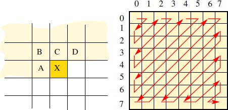
Figure 8.3. Left: in predictive coding, pixel X is coded using neighbors which have already been transmitted: A, B, C, D. Right: zigzag scanning order for a DCT window during JPEG coding
8.5.2. The TIFF format
The TIFF format has already been mentioned in connection with the EP extension, which allows it to handle native formats. In this section, we will consider TIFF itself. Owned by Adobe, TIFF was specifically designed for scanned documents used in graphic arts, which evolved progressively from handling binary documents to handling high-definition color documents. Intended as a “container” format for use in conserving documents of varying forms (vector graphics, text, scanned imaged coded with or without loss, etc.), TIFF is an ideal format for archiving and file exchange, guaranteeing the quality of source documents used with other files to create a final document.
TIFF files are made up of blocks of code, identified by tags, where each block specifies data content. Tags are coded on 16 bits. Above 32,000, tags are assigned to companies or organizations for collective requirements. Tags from 65 000 to 65 535 may be specified by users for private applications. There are therefore a number of variations of TIFF, not all of which are fully compatible. The basic version available in 2015, version 6.0, was created over 20 years ago; this version indicates essential points which must be respected in order to ensure inter-system compatibility. TIFF allows very different structures to be contained within a single image: subfiles, bands or tiles, each with their own specific characteristics to enable coexistence.
Algorithms used to read TIFF files must be able to decode lossless Huffman coding by range and JPEG coding by DCT, and, in some cases, other compression methods (such as LZW and wavelet JPEG), as specific flags and tags are used for these compression types.
TIFF recognizes color images created using RGB, YCbCr or CIE la*b*, coded on 24 bits, or of the CMYK type, coded on 32 bits (see chapter 5). Extensions have been developed for images using more than 8 bits per channel and for very large images.
As a general rule, the TIFF file associated with an image is relatively large. In the case of an image of n pixels in sRVB (3 bytes per pixel), a TIFF file using exactly 1 byte per channel will take up 3n bytes before lossless compression, and around half this value after compression; however, compression is only carried out if requested by the user, making the method slower.
8.5.3. The GIF format
The GIF format is also lossless, and also a commercial product, maintained by CompuServe. While designed for use with graphics, it may also be used to transport images under certain conditions.
GIF is an 8 bit coding method for graphics coded using a color palette, using range-based Lempel-Ziv coding. Black and white images are therefore transmitted with little alteration using a transparent palette (although a certain number of gray levels are often reserved for minimum graphic representation), but with a low compression rate. Color images must be highly quantized (in which case lossless compression is impossible) or split into sections, each with its own palette, limited to 256 colors. Performance in terms of compression is lower in the latter case. Another solution uses the dithering technique, which replaces small uniform blocks of pixels with a mixture of pixels taken from the palette.
8.6. Lossy compression formats
As we have seen, the space gained using lossless image compression is relatively limited. In the best cases, the gain is of factor 2 for a black and white image, factor 3 for a color image or a factor between 5 and 10 for an image coded on 3 × 16 bits.
However, images can be subjected to minor modifications, via an irreversible coding process, without significant changes to their appearance. This approach exploits the ability of the visual system to tolerate reproduction faults in cases where the signal is sufficiently complex (via the masking effect), i.e. in textured areas and around contours.
This idea formed the basis for the earliest lossy coding approaches, which use the same methods described above: predictive coding or coding by run-lengthes or zones. In this case, however, a certain level of approximation is permitted, allowing us to represent a signal using longer strings. Although these approaches are sophisticated, they do not provide sufficiently high compression rates. As a result, new methods have been developed, which make use of the high levels of spatial duplication across relatively large image blocks, projecting images onto bases of specially-created functions in order to group the energy into a small number of coefficients. These bases include the Fourier transformation (especially the DCT variation) and wavelet transformation [BAR 03b].
For any type of lossy coding, users have access to a parameter α which may be adjusted to specify a desired quality/compression compromise. This compromise is highly approximate, and highly dependent on the image in question. The objective criteria used to judge the effects of compression processes were discussed in detail in Chapter 6. Taking I (i, j) to represent the image before coding and I′(i, j) the image after coding, the most widespread measures are:
- 1) compression rate:
- 2) the mean quadratic coding error:
- 3) the signal-to-noise ratio:

- 4) and the peak signal-to-noise ratio:

8.6.1. JPEG
In the 1980s, a group of researchers began work on the creation of an effective standard for lossy compression. This goal was attained in the 1990s, and JPEG (joint photographic expert group) format was standardized in 1992, under the name ISO/IEC 10918-1. The standard leaves software developers a considerable amount of freedom, and variations of the coding program exist. The only constraint is that decoding programs must be able to read a prescribed set of test images [GUI 03b].
8.6.1.1. Principles of JPEG encoding
JPEG encoding is a six-step process, involving:
- 1) a color space change to convert the signal, generally presented in the RGB space, into a luminance/chrominance space (generally YCrCb);
- 2) subsampling of chrominance components using a variable factor, up to 4 in x and y, but usually 2 (this step uses the fact that the eye is less sensitive to fluctuations in color than to fluctuations in gray levels);
- 3) division of the image into fixed-size blocks: 8 × 8 pixels for luminance images, 16 × 16 pixels for chrominance images;
- 4) transformation of these blocks using an operator which “concentrates” the energy of each block into a small number of coefficients, in this case the DCT (discrete cosine transform);
- 5) quantization of these coefficients in order to reduce their entropy;
- 6) transmission of the reordered coefficients by zigzag scanning of the window, followed by Lempel-Ziv coding of the bit chain.
Each of these steps is reversed during the decoding process, with the exception of steps 2 and 5, which involve irreversible information loss.
The direct cosine transform, defined by the matrix in Table 8.1, is a variation of the Fourier transform, which is better suited to real, positive signals, such as images, than the Fourier transform itself [AHM 74]. The DCT is a 2D, exact and reversible transformation of a scalar signal, which creates a real signal with as many samples as the input signal.
Let J(i,j) be a window of N × N pixels (where N = 8, for example) of the channel being transmitted (the luminance or chrominance channel of the original image). The DCT KJ of J is given by:

where ![]() and C(i, i ≠ 0) = 1.
and C(i, i ≠ 0) = 1.
The reverse transformation:

allows us to retrieve the exact value J(i, j), as long as KJ(k, l) has not been subjected to quantization.
Variables k and l are spatial frequencies, as in the case of a Fourier transform. The pair (k = 0, l = 0) has a frequency of zero (i.e. the mean value of J(i, j) for the window to within factor N). As k increases, the horizontal frequencies increase. As l increases, so do the vertical frequencies, and all pair values (k, l) where k ≠ 0, l = 0 corresponds to a frequency which is inclined in relation to the axes 0x and 0y.
The term KJ(0, 0), known as the continuous component, is always much larger than the others. It is treated separately in the DCT, and often transmitted without alterations in order to provide exact, if not precise, information regarding the value of the block.
Table 8.1. DCT filter coefficients for N = 8. Lines: i, columns: k (equation [8.1])
| 0 | 1 | 2 | 3 | 4 | 5 | 6 | 7 | |
| 0 | 1.000 | 1.000 | 1.000 | 1.000 | 1.000 | 1.000 | 1.000 | 1.000 |
| 1 | 0.981 | 0.831 | 0.556 | 0.195 | -0.195 | -0.556 | -0.831 | -0.981 |
| 2 | 0.924 | 0.383 | -0.383 | -0.924 | -0.924 | -0.383 | 0.383 | 0.924 |
| 3 | 0.831 | -0.195 | -0.981 | -0.556 | 0.556 | 0.981 | 0.195 | -0.831 |
| 4 | 0.707 | -0.707 | -0.707 | 0.707 | 0.707 | -0.707 | -0.707 | 0.707 |
| 5 | 0.556 | -0.981 | 0.195 | 0.831 | -0.831 | -0.195 | 0.981 | -0.556 |
| 6 | 0.383 | -0.924 | 0.924 | -0.383 | -0.383 | 0.924 | -0.924 | 0.383 |
| 7 | 0.195 | -0.556 | 0.831 | -0.981 | 0.981 | -0.831 | 0.556 | -0.195 |
The other terms are subject to quantization, to a greater or lesser extent depending on the desired compression rate. We begin by defining a quantizer q(k,l) and an approximation of coefficient KJ(k, l) using ![]() such that:
such that:
where ![]() denotes the default rounded integer value of x.
denotes the default rounded integer value of x.
The set of coefficients q(k, l) thus forms a quantization matrix ![]() which is applied to the whole image. This matrix is transmitted with the associated coefficients in order to enable reconstruction of the image. Coders differ in the way in which they use chrominance subsampling and in the choice of quantization matrices.
which is applied to the whole image. This matrix is transmitted with the associated coefficients in order to enable reconstruction of the image. Coders differ in the way in which they use chrominance subsampling and in the choice of quantization matrices.
As a general rule, high frequency terms can be shown to contain very little energy, and these terms are therefore of limited importance in terms of the perceived quality of the image. These terms are set to zero during quantization (see Figure 8.4 and Table 8.1).

Figure 8.4. Two thumbnails taken from the central image (top left corner). The DCT transforms of the images, after decimation, are given in Table 8.2 (note that gray levels have been amplified in the display process for ease of reading)
Table 8.2. DCT coefficients of thumbnails 1 (left) and 2 (right), after setting all coefficients with an absolute value less than 30 to zero. Note the importance of the term J(0, 0), corresponding to the mean value of the block, and the amplitude of the vertical (in 1) and horizontal (in 2) spatial frequencies corresponding to the periodicities observed in these images
| 0 | 1 | 2 | 3 | 4 | 5 | 6 | 7 | 0 | 1 | 2 | 3 | 4 | 5 | 6 | 7 | ||
| 0 | 1450 | 65 | 0 | 0 | 0 | 0 | 0 | 0 | 980 | 100 | 0 | 0 | 0 | 0 | 0 | 0 | |
| 1 | 0 | 0 | 0 | 0 | 0 | 0 | 0 | 0 | 0 | 0 | 60 | 200 | 0 | 0 | 0 | 0 | |
| 2 | 0 | 0 | 0 | 0 | 0 | 0 | 0 | 0 | 0 | 0 | 0 | 0 | 0 | 0 | 0 | 0 | |
| 3 | 0 | 0 | 0 | 0 | 0 | 0 | 0 | 0 | 0 | 0 | 0 | 0 | 0 | 0 | 0 | 0 | |
| 4 | 0 | 0 | 0 | 0 | 0 | 0 | 0 | 0 | 0 | 0 | 0 | 0 | 0 | 0 | 0 | 0 | |
| 5 | 131 | 0 | 0 | 0 | 0 | 0 | 0 | 0 | 0 | 0 | 0 | 0 | 0 | 0 | 0 | 0 | |
| 6 | 0 | 0 | 0 | 0 | 0 | 0 | 0 | 0 | 0 | 0 | 0 | 0 | 0 | 0 | 0 | 0 | |
| 7 | 0 | 0 | 0 | 0 | 0 | 0 | 0 | 0 | 0 | 0 | 0 | 0 | 0 | 0 | 0 | 0 |
The coefficients ![]() are then transmitted by zigzag scanning, which places frequencies in increasing 2D order (as far as possible) after the continuous component (see Figure 8.3, right). After a short period, the coefficient string will only contain zeros, which will be compressed effectively using either Liv-Zempel or range-based Huffman techniques.
are then transmitted by zigzag scanning, which places frequencies in increasing 2D order (as far as possible) after the continuous component (see Figure 8.3, right). After a short period, the coefficient string will only contain zeros, which will be compressed effectively using either Liv-Zempel or range-based Huffman techniques.
JPEG images are decompressed by reversing all of the steps described above. Coefficient quantization can highlight faults in individual blocks which are characteristic of the JPEG format. Certain reconstruction algorithms therefore include a low-pass filtering stage which reduces these faults. The subsampling of chromatic components may also require an additional interpolation stage, which may also have damaging effects on the image.
8.6.1.2. JPEG in practice
JPEG compression has become the most widely accepted means of transmitting images of reasonable quality and reasonable volume. For color images, a compression rate of 10 is generally considered to cause very little degradation to the image, practically imperceptible to the naked eye, especially for very large image files and when viewed without excessive magnification.
Compression rates of 100 are also widely used, particularly online or when sending images by email. Image quality is highly compromised in this case, and the images in question cease to be suitable for any use except rapid visualization due to the presence of annoying artifacts.
Note that all encoders include a parameter to control compression rates, and this parameter is often unique. However, this indicator is not formally connected to compression gains or to image quality. Applied to two different images, the same index may produce two very different results. For a single image, as the index decreases, the level of degradation and the compression rate increase. This index generally takes a value of 100 in the case of lossless coding, and may be reduced to a minimum value of 1.
Note, however, that lossless JPEG does not use the general principle of the DCT for encoding purposes, as it is based on predictive methods.
JPEG may be used in a progressive manner for transmission purposes: in this case, low frequency terms are transmitted first, and the image is then refined by the transmission of higher frequencies.
A version of the image made up of continuous components alone, 64 times smaller than the original, is often used for display functions or to enable rapid database searches.
8.6.2. JPEG 2000
The JPEG 2000 standard is recognized by the ISO under the name ISO/IEC 15444-1, and is a relatively general image exchange standard, offering a variety of functions (archiving, internet and video). In this context, we will focus on the aspects relating to the image format.

Figure 8.5. Magnification of an area of an image encoded using JPEG. The top left image is the non-encoded original. The whole image has then been compressed by factors of 5.4 (top right), 12.1 and 20 (central line), and 30 and 40 (bottom line). For a color version of this figure, see www.iste.co.uk/maitre/pixel.zip
JPEG 2000 makes use of the fact that wavelet composition offers better performances than the DCT in terms of image compression: this method provides a better quality image than DCT with the same compression rate, and higher compression rates for the same image quality [BAR 03a].
JPEG 2000 is also scalable.
The format also uses a highly developed arithmetic encoder, EBCOT (embedded block coding with optimized truncation) which makes use of the 2D tree structure of the wavelet decomposition [TAU 00].
Finally, JPEG 2000 gives users the possibility to describe image content at a higher level of the pyramid; this is useful in facilitating intelligent use of image collections, and for optimized transmission over new-generation networks. To do this, the format makes use of the progressive transmission capabilities offered by wavelet scalability, via a codestream transmission structure, and the ability to define regions of interest (ROI) which are transmitted first and with higher quality levels. It explicitly accounts for the possible presence of text or graphics in compound structures. The format is also designed for application to very large images (up to 232 pixels per line), images with a large number of channels (up to 214) and images with high-dynamic pixels (up to 38 bits per sample).
As with many other standards, JPEG 2000 is open and does not explicitly specify a compression mode, leaving developers the freedom to make improvements over time. The encoder is obliged to produce a binary string which conforms to the standard, but any strategy may be used to do this. Decoders must simply prove their ability to decode the example files included with the standard.
As a transmission standard, JPEG 2000 is highly suited to professional requirements. It has had less success with the general public; its requirements in terms of calculation power and decoding software are higher than those of JPEG, but this is of minor importance compared to the effects of inertia in the general market, where users are not overly concerned with obtaining high quality/flux ratios.
8.6.2.1. Principles of JPEG 2000
Like JPEG, JPEG 2000 is able to transform color images created using the RGB space into a luminance/chrominance space (YUV or Y CRCB). Two types of transformations are available, one reversible, the other irreversible (but more effective in terms of compact representation). The chromatic components are then processed separately.
JPEG 2000 then operates either on the image as a whole, or on tiles, identically-sized sections of the image (with the exception of the edge tiles). These tiles are decomposed hierarchically by a bank of 2D, bi-orthogonal wavelet filters [BAR 03a].
The standard allows the use of two types of filters13:
- 1) Le Gall 5/3 rational coefficient filters, as discussed in section 8.4; these filters only operate using rounded integers, and may be used for lossy or lossless coding, depending on whether all of the non-null coefficients are transmitted (using the EBCOT method, described below),
- 2) Daubechies 9/7 real coefficient filters14 (see Table 8.3), which can only be used for lossy coding, as calculations are carried out using real numbers with a finite level of precision. These wavelets perform better than rational wavelets in the context of lossy coding.

Figure 8.6. Lifting diagram for 3 levels of n, n + 1 and n + 2 wavelet decomposition, showing the separation of odd and even samples. The differences between odd samples and their predictions, made on the basis of the even samples, are known as level n details. The risk of aliasing is taken into account by filtering the detail signal and reinserting it into the even samples, which are then used to form a signal of level n+ 1. The lifting process may then be applied to the signal, and so on, until the required depth is reached
These filters are bi-orthogonal15, and defined by a low-pass filter used to calculate images with increasingly low resolutions, starting from the original level of the tile, and a high-pass filter, used to define the contents of details characterizing the specific level in question. These details are contained within the coefficients of the wavelet decomposition: an(i, j).
Filtering can be carried out in two ways. The first method, using convolution, is that generally used in signal processing as a whole. The second method, which constitutes a major advantage of the hierarchical wavelet approach, involves the iterative application of two filters, one low-pass, the other high-pass; these filters are identical for all levels of the pyramid. This is known as the lifting process. Using this process (see Figure 8.6), the odd coefficients of a decomposition are expressed using the value of the even coefficients with the application of a corrective term. This corrective term constitutes the specific detail image for the level in question [SWE 96].
The basic wavelet transformation is one-dimensional (1D); it is thus applied once to the lines and once to the columns of the area of interest. This results in the production of 4 images (see Figure 8.7):
- – an image with high frequencies in both lines and columns;
- – an image with high frequencies in the lines and low frequencies in the columns;
- – an image with high frequencies in the columns and low frequencies in the lines;
- – an image with low frequencies in both lines and columns.
In a carefully-chosen wavelet base, these coefficients present a number of interesting statistical properties; they are highly concentrated, and can be efficiently modeled using a generalized Gaussian law, allowing efficient quantization:
Quantization tables are defined for each resolution level, and calculated in such a way as to provide a wide range of compression levels.
These quantized coefficients, transformed into bit planes and grouped into subbands, are then transmitted to the encoder. As we have seen, the EBCOT coder uses a high-performance contextual encoding process involving a wavelet coefficient tree, predicting each bit using the same bit from the previous resolution level and its immediate neighbors, starting with those bits with the heaviest weighting. The encoder processes subblocks, which are relatively small (with a maximum 64 × 64); the precise size of these subblocks is defined by the user.
The power of the coding method is based on the domain of hierarchical analysis of the wavelet decomposition. We will consider neighborhoods of 6 or 27 connections within a three-dimensional (3D) pyramid of resolution levels. The majority pixels (identified by the bit from the previous level) are not encoded; the others are coded using their sign and deviation from the previous level, if this is significant. Finally, we consider situations where there is no dominant configuration. The resulting tree structure is encoded using an algebraic code.
Table 8.3. Coefficients of Daubechies 9/7 wavelet filters for image analysis and reconstruction (based on [BAR 03a]). Note that other formulas exist, which differ by a factor √2. The analysis and reconstruction filters need to be symmetrical in relation to order 0 to avoid moving image contours
| order of filter | 0 | ± 1 | ± 2 | ± 3 | ± 4 |
| analysis: low-pass filter | 0.602949 | 0.266864 | -0.078223 | -0.016864 | 0.026749 |
| analysis: high-pass filter | 0.557543 | 0.295636 | -0.028772 | -0.045636 | 0 |
| synthesis: low-pass filter | 0.602949 | -0.266864 | -0.078223 | 0.016864 | 0.026749 |
| synthesis: high-pass filter | 0.557543 | -0.295636 | -0.028772 | 0.045636 | 0 |
8.6.2.2. JPEG 2000: performance
The compression rates obtained using JPEG 2000 are around 20% higher than those for JPEG for the transmission of fixed images of identical quality. Subjectively speaking, the drawbacks of JPEG 2000 are less problematic than those encountered using JPEG, as the systematic block effect no longer occurs. JPEG is particularly effective for very large images, along with images containing few very high frequencies. JPEG 2000 produces satisfactory results for high compression levels (of the order of 100). The standard is also highly adapted for remote sensing images, due to its ability to process large images using a mode compatible with the tiling approach needed for high-resolution navigation, and to the possibility of specifying zones of interest, which are then subject to greater attention.
8.7. Tiled formats
To complete our discussion of fixed image coding, let us consider the case of very large images. This situation is not yet widely encountered in photography, but with the development of sensors of 50 megapixels and more, these formats may be used by certain devices in the relatively near future.
Tiled formats are used for very large image files (from 10 megapixels up to several gigapixels) and are designed to allow rapid consultation of these images. The images in question are decomposed into tiles (with a default size of 64 × 64 pixels in FlashPix, the most common form, and 256 × 256 pixels in the IVUE format). They also use a pyramid shaped, hierarchical binary description of the image, moving from full resolution (several hundred tiles) to a single, coarse image contained in a single tile. A pixel at any level of the pyramid is obtained by averaging the four pixels from the previous level which it is intended to represent. The use of a tree structure allows rapid determination of the level of representation required in response to a user request (for example to display a zone of a given size on a screen of a given size). The use of this tree, along with pre-calculated representation structures, allows very significant gains to be made in terms of image manipulation, both for input/output purposes and for processing, for example when scrolling across a screen.
The payoff for this gain is an increase in the required storage space, as the original image (split into small tiles) needs to be conserved, alongside versions at 1/2, 1/4, 1/8 resolution etc.; this gives a total storage space of ![]() times the size of the image, ignoring possible truncation errors, i.e. a 33% increase in memory requirements.
times the size of the image, ignoring possible truncation errors, i.e. a 33% increase in memory requirements.
The FlashPix format is able to handle tiles of any type: 8 or 16 bits, 1, 3 or 4 channels, coded using lossy or lossless methods. A description of the Flashpix representation (tile size and number) is given in the associated EXIF file.
Plane representations are replaced by spherical forms in the context of very large datasets, such as those used in astronomy and remote sensing. In this case, a specific tiled representation of the sphere is required. The best-known example, HEALPix (hierarchical equal area isolatitude projection of a sphere) [HEA 14], decomposes the sphere by projection onto 12 squares of a plane, set out in a staggered formation, using different projections according to the position of the zones in question. These squares are oriented at π/2 in relation to the equator, and centered on either (0, kπ/2) or (kπ/4, ±π/4). The resulting squares are then split into 4, following a classic hierarchical approach.
A more intuitive form of tiled projection, hierarchical triangular mesh (HTM) [KUN 01] decomposes the sphere into triangles along large circular planes of the sphere; another format, QuadTree Cube (Q3C) simply uses the quadratic hierarchical structure [KOP 06].

Figure 8.7. Image coding using JPEG 2000. Top left: level 2 image, with 3 level 1 detail images: top right, detail resulting from a low-pass horizontal filter and a high-pass vertical filter; bottom left: detail resulting from a transposed filter: horizontal high-pass, vertical low-pass; bottom right: result of a low-pass vertical filter and a high-pass horizontal filter. Properly combined, these four images give the original image (using the Daubechies wavelet base)
These tiled representations of spherical forms are particularly useful in photographic assemblies and in panoramas with very wide fields (see section 10.1.8).
8.8. Video coding
The domain of video encoding lies outside the scope of this work; however, an increasing number of cameras allow users to record both fixed images and moving sequences. These cameras include video encoding elements which compress the image flux. As in the case of fixed images, these encoders exploit the duplications within each image (intra-image coding), but also duplications between successive images (inter-image coding).
8.8.1. Video encoding and standardization
Standardization work has been carried out by the ITU16, producing recommendations H.120, H.261, H.263 and H.264. The H263 standard was the first to include an inter-image mode; H264 serves as the basis for MPEG-4.
These recommendations have also been used outside of the field of telecommunications, for applications such as archiving, video games and private usage. The moving picture expert group (MPEG) committee, a joint venture by the ISO and the IEC, has worked on creating consensus solutions for the purposes of standardization [NIC 03].
The first recommendation, MPEG-1, concerned low flow rate transmissions for wired transmissions in the period preceding ADSL (using packets of 64 kbit/s, giving a maximum rate of around 1.5 Mbit/s). This very low rate was only suitable for video transmission of very small images (352 × 288 pixels per image at a rate of 25 image/s). MPEG-1 was widely used in the context of video-CD archiving.
The MPEG-2 standard was designed for television, and specifically for high quality transmission (contribution coding). It is particularly suitable for Hertz transmission, whether via cable or ADSL. The standard allows transmissions of between 2 and 6 Mbit/s for ordinary video and of 15 to 20 Mbit/s for HDTV17.
MPEG-4 is a multimedia transmission standard, part of which deals specifically with video images. It is particularly concerned with low-rate transmission (around 2 Mbit/s) and uses more elaborate compression mechanisms than those found in MPEG-2; these mechanisms are suitable for use with highly compressed files (although a significant reduction in quality is to be expected). MPEG-4 makes use of the scalability properties included in recommendation H.263. It forms the basis for easy communications with the field of computer science, particularly with regard to copyright protection.
Developments MPEG-7, MPEG-21 and MPEG-x (with x taking a value from A to V) are designed for multimedia applications of video sequences, and define specific functions for archiving, database searches, production (particularly the integration of a variety of sources), interaction, diffusion and content protection.
8.8.2. MPEG coding
8.8.2.1. Mechanisms used in MPEG
The video coding standards contained in MPEG-2 and MPEG-4 are currently used in many cameras. Architectures designed for vector-based treatment and integrated into the camera are used to carry out weighty calculation processes, using many of the elements of these standards [NIC 03, PER 02].
We will begin by considering the implementation of MPEG-2. A color image, generally acquired in a RGB space, is converted into a {luminance, chrominance} space, and the chrominance channels are generally subsampled using a factor of 2 for both lines and columns, as in the case of JPEG.
Intra-image coding is carried out by subdividing the image into groups of blocks (GOB), constructed from macroblocks, MB. A macroblock is itself made up of 4 blocks of 8 × 8 pixels of luminance and, generally, 1 chrominance block (chroma subsampling encoding, 4 : 2 : 0) or 4 blocks (in the case of 4 : 4 : 4 encoding, without subsampling). The binary string is therefore made up of an image layer (I), made up of layers of groups of blocks (GOB), themselves made up of macroblock (MOB) layers. This macroblock layer typically includes the 4 luminance blocks followed by 2 chrominance blocks, one for dominant R, one for dominant B.
These blocks are coded using a discrete cosine transformation (DCT) quantizied, then subjected to entropic encoding (by range length, or, better, arithmetic coding) (Figure 8.8).

Figure 8.8. Diagram showing the principle of image encoding in an H.262 flux. Either intra-image or predictive mode may be used. DCT is the cosine transformation of a block of 8 × 8, and DCT−1 is the reverse transformation. Q is a quantizer and Q−1 is the dequantizer. LVC is a variable-length range coder. The lower left box is the movement predictor. The movement detection stage is followed by movement compensation, used to measure the prediction error, coded in the block using the DCT. The decision to switch to inter- or intra-image mode is based on the position of the image in the flux
There are two possible modes of inter-image encoding:
- 1) predictive mode (mode P): one image from the flux is taken as a reference and transmitted with intra-image encoding (image I). The new image (P), to be transmitted later, is compared to I in order to determine the movement affecting each pixel. This movement prediction stage operates using block matching, and determines a movement vector (Δx in x and Δy in y) for each macroblock. The difference between the macroblock in image P and that in image I, offset by {Δx, Δy}, constitutes an error macroblock, which is encoded using the DCT. The image is transmitted by sending the address of the reference macroblock in I, the movement vector {Δx, Δy}, and the error block, quantized and entropically compressed.
- 2) bidirectional interpolated mode (mode B): using this mode, the image flux is interpolated using both an earlier image I and a later image P
to reconstruct intermediate images noted B (see Figure 8.9) using a very small quantity of additional transmission space (only elements essential for positioning the macroblock in B are added, in cases where this cannot be deduced by simple interpolation of that of P). However, this operating mode does result in a delay in image reconstruction; for this reason, it is mostly used for archiving purposes, where real time operation is not essential, or in applications where a very low level of latency will be tolerated.
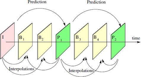
Figure 8.9. Coding an image flow using MPEG: I is the reference image, coded as an intra-image. P1 and P2 are images coded by movement prediction based on I, and on P1 and I in the case of P2. B1 and B2 are interpolated from I and P1, and B3 and B4 are interpolated from P1 and P2
This coding mode generates significant block effects in the case of high compression rates. A number of improvements have been proposed to eliminate this issue: multiplication of movement vectors for each macroblock, block layering when identifying movement, a posteriori filtering, etc.
In MPEG-4, most of the functions of MPEG-2 described above have been improved: better prediction of DCT coefficients, better movement prediction, resynchronization of the data flux, variable length entropic coding, error correction, etc. Part 10 of the standard introduces a new object, the VOP (video object plane), a box surrounding an object of interest. A VOP may be subjected to a specific compression mode different to that used for the rest of the image. A VOP is made up of a number of whole macroblocks, and will be identified in the data flux. For example, a participant in a television program, speaking against a fixed background, may be placed into a VOP with high definition and a high refresh frequency, while the studio background will be coded at a very low rate. VOPs, generally described on an individual basis by users, are not currently used in most cameras (which tend to focus on part 2 of the MPEG-4 recommendations). However, certain cameras now include very similar functions (for example higher-quality coding in a rectangular zone defined by facial recognition).
The use of MPEG-4 coders in cameras and their ability to encode high definition videos (HDTV format18, in 2015, with 4k format available on certain prototypes for durations of a few seconds) represents a major development in camera technology, as this application currently determines the peak processing power, defines the processor and signal processing architecture, the data bus and the buffer memory.
8.9. Compressed sensing
No chapter on image encoding and compression would be complete without at least a rapid overview of this technique, which, in 2015, shows considerable promise in reducing the volume of image signals beyond the possibilities offered by JPEG 2000. However, compressed sensing is still a long way from constituting a standard or an image forward, and does not yet constitute a reasonable alternative to the standards discussed above [ELD 12].
The basic idea in compressed sensing is the reconstruction of images using a very small number of samples, notably inferior to the number recommended by the Shannon theorem19 [DON 06, BAR 07, CAN 08]. The proposed approaches consist of applying a number of relevant and complementary measures in order to reconstruct the image using sophisticated techniques which make use of the sparsity of image signals, essentially by using reconstructions of norm ![]() 0 or
0 or ![]() 1. Sparsity is the capacity of a signal for description in an appropriate base exclusively using a small number of non-null coefficients. Image sparsity cannot be demonstrated, and is not easy to establish. The hypothesis is supported by strong arguments and convincing experimental results, but still needs to be reinforced and defined on a case-by-case basis.
1. Sparsity is the capacity of a signal for description in an appropriate base exclusively using a small number of non-null coefficients. Image sparsity cannot be demonstrated, and is not easy to establish. The hypothesis is supported by strong arguments and convincing experimental results, but still needs to be reinforced and defined on a case-by-case basis.
Compressed sensing places image acquisition at the heart of the compression problem; this approach is very different to that used in sensors which focus on regular and dense sampling of whole images, using steps of identical size. However, this “Shannon style” sampling is not necessarily incompatible with all potential developments in compressed sensing. The onboard processor is left to calculate the compressed form in these cases, something which might be carried out directly by sophisticated sensors (although this remains hypothetical in the context of everyday photography).
Presuming that an image can be decomposed using a very small number of coefficients in an appropriate base, we must now consider the best strategy for identifying active coefficients. Candès and Tao have shown [CAN 06] that images should be analyzed using the most “orthogonal” measurement samples available for the selected base functions, so that even a small number of analysis points is guaranteed to demonstrate the effects of the base functions. As we do not know which base functions are active, Candès suggests using a family of independent, random samples [CAN 08]. Elsewhere, Donoho specified conditions for reconstruction in terms of the number of samples required as a function of signal sparsity [DON 09].
In terms of base selection, no single optimal choice currently exists, but there are a certain number of possibilities: Fourier bases, DCT, wavelets (as in the case of JPEG) and wavelet packets used in image processing (curvelets, bandlets, etc.). Reconstruction with a given basis is then relatively straightforward. This process involves cumbersome optimization calculations using a sparsity constraint, for example by searching for the most relevant base function from those available, removing the contributions it explains from the sample, and repeating the process (the classic matching pursuit algorithm [MAL 93]), or by convex optimization.
If an image is principally intended for transmission, reconstruction is not desirable; we therefore need to consider the transmission of random samples. The random character of these samples is not helpful in ensuring efficient transmission, and imposes serious limits on the possible performance of the compressed sensing process, unless we use certain well-mastered quantization and coding forms [GOY 08]. Other types of representation would therefore be useful, and development of these forms is important in order to derive full profit from compressed sensing techniques; however, a lot of work still needs to be done in this area.
Current studies of compressed sensing have yet to produce results of any significance for mass market photography. However, an innovative prototype of a single-pixel camera has been developed, tested [DUA 08] and marketed by InView. This prototype captures images using a matrix of mirrors, individually oriented along both the x and y axes, in order to observe a different aspect of the scene at each instant. All of the signals sent by the mirrors are received by a single sensor, which produces a single pixel for any given instant, made up of a complex mixture of all of these signals. The matrix is then modified following a random law and a new pixel is measured. The flux of successive pixels, measured at a rate of around 1,000 pixels per second, is subjected to a suitable wavelet-based reconstruction process in order to recreate the scene, using around one tenth of the samples previously required. This technology is particularly promising for specific wavelengths for which sensors are extremely expensive (for example infra-red, a main focus of the InView marketing strategy).
Compressed sensing applications are particularly widely used in the field of instrumentation, where they have provided interesting solutions to complex 3D measurement problems in medical imaging (axial tomography, magnetic resonance etc. [LUS 08]), in microscopy for biological purposes [LEM 12], in holography and for physical instrumentation [DEN 09], etc.
For photographers, compressed sensing is a promising area, but considerable developments are required before these methods are suitable for general use.