
9
Elements of Camera Hardware
This chapter will cover most of the components found in camera hardware, with the exception of the lens (discussed in Chapter 2) and the sensor (Chapter 3). We will begin by describing the internal computer, followed by memory, both internal and removable; screens, used for image visualization and for modifying settings; shutters, focus and light measurement mechanisms; image stabilization elements; additional components which may be added to the objective, including rings, filters and lenses; and, finally, batteries.
9.1. Image processors
The processors used in camera hardware have gained in importance over time. The high-treatment capacities required in order to format sensor output signals and to control all of the functions affecting photographic quality have resulted in significant changes to the camera design process. Big-name brands, which have occupied large portions of the market due to their high-quality optic designs and ergonomic hardware elements, found themselves needing to recruit electronics specialists, followed by specialist microcomputing engineers. New actors, mainly from the domain of mass-market audiovisual technology, have also emerged onto the market, often by buying existing brands which were struggling to find the necessary funds to invest in mastering these new technologies. Above and beyond image processing, new functions have been added to cameras, preparing data for storage and printing, using geolocation technology or Internet capabilities, incorporating elements from the field of computer science (such as touch screens) and from the domain of telecommunications.
In the past, the processor market and the optical photography market were two distinct entities. High-quality objective designs were intended to be used over a period of 20 years or more, and used alongside or as an addition to existing products. Microprocessors, on the other hand, evolve rapidly: manufacturers change processor design around once every 3 years, and each new element is intended to replace its predecessors across the whole range. The processor is not designed for a specific camera, and is intended to provide the required performances for a wide variety of purposes in terms of processing speed, input parallelization, memory access, communications facilities, etc. These performances are generally all utilized in high-end professional reflex cameras, which act to showcase the skills and capacities of manufacturers. They are then used to a lesser extent by other models in the range, designed for specific purposes, whether prioritizing video capture, optimizing everyday processing, operating in difficult conditions or ensuring Internet connectivity. In these cases, specific programs are added to the processor, defining the performances and capacities of the camera. These programs are responsible for activating specific processor functions which associate specific sensor measurements with specific settings. The potential of any camera is thus defined by the sensor, processor and software combinations used, all of which are placed at the service of optical components.
9.1.1. Global architecture and functions
As we have stated, all of the big players in the camera market maintain their own range of processors: Canon uses the Digic range; Nikon, Expeed; Sony, Bionz; Olympus, TruePic; Panasonic, Venus; Pentax, Prime; and Samsung, DRIMe. However, these products are often developed in collaboration with integration specialists, for example Texas Instruments or Fujitsu, to design cores based on non-proprietary image processing circuits. The processor itself is then completed and integrated by the manufacturer, or co-designed in the context of specific manufacturer/specialist partnerships. For instance, Fujitsu is responsible for the creation and continued development of the Milbeaut architecture, which is included in a wide variety of processors (probably including those used by Leica, Pentax and Sigma) and forms the basis for Nikon’s Expeed processors. Texas Instruments worked in partnership with Canon to develop Digic processors, based on their integrated OMAP processor. A smaller number of manufacturers deal with all aspects of component design in-house, including Panasonic, Sony and Samsung. However, the convergence of photography with cellular telephony has led to the integration of increasingly powerful components, with increasingly varied applications outside of the field of optical imaging, and specialized architectures for camera processors are now becoming obsolete1.
We will not go into detail here regarding the image processors used in camera cores; as we have seen, architectures evolve rapidly, and today’s state-of-the-art elements may be obsolete tomorrow. Moreover, hardware configurations are also extremely variable; while most modern cameras include a central processing unit (CPU) associated with a digital signal processor (DSP), some examples also include graphic processors, multiple CPUs or multi-core CPUs with distributed operations. This is particularly true of high-end models, which have higher requirements in terms of processing power. Evidently, the payoff for this increased power is an increase in electrical power requirements, resulting in reduced autonomy. However, this issue lies outside of the processing domain.
Figure 9.1 shows the key elements with requirements in terms of processing power:
- – electronic cycle controls, which allow the sensor to acquire images;
- – processing the signal recorded by the sensor, transforming it into an image and recording it on the memory card;
- – management of signals from a variety of measurement instruments: user settings, photometers, telemeters, battery level, memory state, gyroscope or ground positioning systems (GPS) where applicable; power is also required to alter camera settings, including the diaphragm aperture, focus adjustment and flash;
- – communication with the user (program management and menu navigation, image display, memory navigation, etc.) and user interface management (program selection, measurement zone displays, parameters, signal levels, error notifications, etc.).
9.1.2. The central processing unit
The CPUs used in modern cameras offer the same functions as general processing units. They are built using classic architectures (for example, TMS320 for the Texas Instruments family, or the ARM-Cortex A5 in the context of Milbeaut processors), use sophisticated programming languages (for example, a LINUX core in the case of Android platforms) and communication functions using the Internet, BlueTooth or Wifi. While measures are generally taken by manufacturers to prevent users from reprogramming these elements (jailbreaking), a number of open CPUs are available and may be used to host the user’s own developments. Moreover, there is extensive evidence of users tampering with camera CPUs, and a number of smaller companies provide users with a means of integrating their own programs into high-end camera hardware.

Figure 9.1. Operating diagram of an image processor. Processing functions are shared between the CPU and the DSP. Signals produced by the sensors (path a) are processed by the CPU and used to adjust optical parameters (path c). The CPU controls sensor command signals (path b) and the parameters of the DSP (path e). It is also responsible for the user interface. The DSP receives the data flux produced by the sensor, formats the data and transmits it to the memory card for storage. It transmits user dialog elements (signal dynamics, saturated zones, etc.) to the CPU, and often relies on a specialized graphics processor (GPU) for display purposes. Image signals travel through a specialized image bus. Certain cameras also include a buffer memory which is quicker to access than the memory card itself
The CPU is responsible for all high-level camera functions, and is notably responsible for the coordination and sequencing of the functions described above. The CPU also manages the operation of more specialized processors, including the DSP and graphics processing unit (GPU), where applicable.
The CPU takes charge of advanced processing operations, and translates user selections (often expressed in relatively abstract terms: “sport”, “backlight”, “landscape” , etc.) into precise instructions, tailored to the specific capture conditions: choice of sensitivity, aperture and exposure time, along with the means of measuring focus and aperture, white balance where applicable, and flash use. It also determines focal priorities in cases where sensors produce different results (varying measurement zones in the field, simultaneous use of multiple preferential measurements (e.g. multiple faces), target tracking, etc.). While these decisions are generally made using logical decision trees, a number of other solutions have been recently proposed, using statistical learning techniques alongside databases recorded in the camera itself. This method is notably used in the Canon intelligent scene analysis based on photographic space (ISAPS) system, which controls focus, exposure and white balance on the basis of previously-recorded examples.
The CPU also ensures that other components are configured in accordance with its instructions: focus, diaphragm aperture and capture stabilization.
The CPU is responsible for the creation of metadata files (EXIF file and ICC profile) (see section 8.3.2), archiving the image on the memory card, indexing it to allow users to navigate through previous files, and, where applicable, allowing searches by capture date or theme. Up to a point, it is also involved in managing color printing or transmission to a network, either via a universal serial bus (USB) port or using a wireless communication protocol.
Special effects (black and white or sepia imaging, backlighting, solarization, chromatic effects, etc.) and other non-traditional treatments (panoramas, stereovision and image layering) are also handled by the CPU. We will consider a number of examples of this type of process, with the aim of demonstrating their complexity, something which is rarely apparent to the user:
- – Many modern cameras are now able to detect tens of individual faces in a scene, then to select those which seem to be the most important for the purposes of focusing and exposure; these selected faces may also be tracked in burst mode.
- – Certain models produced by Canon and intended for family use include a specific setting mode able to detect a child in the center of a scene. This mode includes 17 different configurations, 13 of which are designed for photographing babies; five of these 13 options are intended for sleeping babies, in a variety of lighting conditions. Four configuration options are specifically designed for children in action, and, once again, use different settings depending on the ambient lighting conditions.
- – The Fujifilm EXR CRP architecture includes a relatively comprehensive scene identification program, which includes not only classic situations (indoor, outdoor, portrait, landscape, flowers, etc.), but can also detect, recognize and track cats and dogs. This information is located within the proprietary area of the EXIF file (see section 8.3.2) and may be used later in the context of keyword searches.
- – In certain configurations, the Olympus TruePic processor applies specific treatments to colors identified as corresponding to human skin and to the sky. These processes operate independently of white balance and are limited to clearly-defined zones in the image, detected and defined prior to processing.
- – Canon uses the ISAPS database to offer different strategies for flash management, used to distinguish between situations in which all faces in a scene need to be clearly visible (for example, at a family party) and situations in which unknown faces should be treated as background (for example, at tourist sites). The use of learning databases is becoming increasingly widespread in optimization strategies, for example, in EXPEED 4 in the Nikon D810.
- – In portrait mode, the BIONZ processor in Sony α products includes facial processing features which focus precisely on the eyes and mouth of the subject, with reduced focus on skin details; this is intended to replace postprocessing improvement operations generally carried out in a laboratory setting.
9.1.3. The digital signal processor
The DSP is an architecture developed specifically for the treatment of image data, using a single instruction multiple data (SIMD) – type pipeline assembly, which repeats the same type of operation multiple times for a very large data flux. It exploits the specific form of calculations involved (using integers, with a reduced number of bits, multiplication by a scalar and addition of successive numbers) to group complex operations into a single operation, applied to long words (128 or 256 bits) in a single clock time (following the VLIV principle: very long instruction word). In cases with higher power requirements, the DSP uses parallelized processing lines, using the multiple instruction multiple data (MIMD) processor architecture, for example using eight parallel treatment paths. The particular structure of images is particularly conducive to this type of parallelization, and processes of this type are easy to transcribe into VLIV instructions.
The DSP collects data output from the photodetector, organizes these data and directs them to various treatment lines. These data can vary considerably depending on the sensor. Note that modern CMOS technology (see Chapter 3) has led to the integration of certain functions in the immediate vicinity of the photosensitive site, including analog/digital conversion, quantization and the removal of certain types of parasitic noise. It has also resulted in the use of specific representation types, in which neighboring pixels are coupled together, either because they share the same electronic component or because they are complementary in terms of representing a particular signal (HDR, stereo or very low-dynamic signals: see Chapter 3). In this case, these processes are applied to data before it reaches the DSP.
The key role of the DSP is to carry out all of the processes required to transform a raw signal into an image for display, generally in JPEG format in sRGB or ICC color mode (see section 5.2.6). Although images are recorded in native (RAW) format, it is essential to give users access to the image in order to monitor the capture process.
A generic example of the series of processes carried out by the DSP is given below:
- – The native signal is corrected to compensate for the dark current (dependent on the exposure time and the temperature of the camera). This current is often estimated using dedicated photosites, outside of the useful image field, on the edge of the sensor. The corresponding level is subtracted from all pixels. Bias introduced during the capture process may also be removed in order to exploit the centered character of thermal noise.
- – Certain field corrections are applied in order to reduce the effects of noise on very weak signals (spatial means) and to reduce chromatic distortions and vignetting, according to the position of each pixel within the image.
- – Initial white balancing may be applied to all signals in order to take account of the spectral response of the sensor and user settings.
- – A demosaicing process is then applied in order to create three separate signals, R, G and B.
- – Gamma correction may be applied, where necessary, in order to take account of nonlinearity in the sensor.
- – Advanced chromatic corrections may also be applied. These may require the use of a perceptual color space, such as Lab and YCrCb (see section 5.2.3), and can affect the white balance carried out previously, due to the use of a global optimization strategy (see section 5.3). These corrections are often followed by a process to filter out false colors, which may be due to the residues of chromatic impairments at the edge of the field, in high-contrast images.
- – Accentuation algorithms can be used in order to fully utilize the chromatic and dynamic palette, increase contrast and improve sharpness (see section 6.1.2).
Specialized functions may involve operations which are extremely costly in terms of machine time: for example, direct cosine transformation (DCT) is required in order to move from an image signal to a JPEG representation, and for the lossless compression procedures used to limit file volume in RAW format (see section 8.4). Other functions are specifically used for video formats: movement prediction and optical flow (discussed in Chapter 10), audio channel processing, etc.
Modern equipment is able to carry out these functions in a very efficient manner, and bursts of over 10 images per second are now possible (if the memory card permits) for most high-quality cameras of 20 megapixels and above. Note that the use of buffer memory allows us to avoid the bottleneck effect limiting the flow of data into an external memory card. However, this memory, in RAM or SDRAM format, as it supports high flow rates (typically from 500 megabits/second to 1 gigabit/second) has a capacity limited to a few images.
The performance of modern DSPs is not limited by the treatment of fixed images, but rather by video processing, much more costly in terms of processing rates. The reference element used in this context is “4k” video, i.e. 4,000 pixels per line in 16/9 format; this format has twice the resolution, in both lines and columns, than the TVHD standard. Coded using the MPEG 4 standard (ISO H264/AVC), it requires the treatment of 30 images per second using full frame resolution (30 ffps), or 60 images per second in interlaced mode (60 ifps), see section 8.8.2. As of 2015, this still represents a challenge for many manufacturers, who continue to use TVHD format (1,920 pixels per line).
9.1.4. The graphics processing unit
In cameras with a graphics processing unit, this element is responsible for displaying images on the camera screen, as well as on the viewfinder, in the case of many hybrid systems where this component is also electronic.
The GPU allows the resolution to be adapted to camera screens, which are generally very small in relation to the size of the image (one megapixel rather than 20). It is responsible for zoom and scrolling functions, and for image rotation (for portrait or landscape visualization). It applies white balancing or special effects in real time, and allows the use of digital zoom to interpolate image pixels between measurement points, for example using bilinear or bicubic interpolation. The GPU also allows the modification of color tables, indicating saturated or blocked zones. It calculates and applies focus histograms and zones, along with all of the graphic or alpha-numeric indications required for user dialog. GPUs are also partly responsible for touch-screen functions in cameras which include this technology.
9.2. Memory
9.2.1. Volatile memory
Cameras generally include a volatile memory, allowing temporary storage of images immediately following capture, before archiving in permanent storage memory. Volatile memory is able to store a small number of images in native (RAW) format, and the capacity of this element defines the maximum limit for camera use in burst mode. These memory elements generally use dynamic random access memory (RAM), or DRAM. They are generally synchronized with the image bus (SDRAM = synchronized dynamic random access memory). Input and output, controlled by the bus clock, can be carried out in parallel, serving several DSP processing banks simultaneously in order to speed up operations.
Live memory (which consists of switches, or transistor-capacitance pairs) requires a constant power supply, and data need to be refreshed during the processing period. It is generally programmed to empty spontaneously into the archive memory via the transfer bus as soon as this bus becomes available. The transfer process may also occur when the camera is switched off, as mechanisms are in place to ensure that a power supply will be available, as long as the memory is charged.
Flow rates, both in terms of reading (from the photodetector or the DSP) and writing (to the DSP) can be in excess of 1 gigabyte per second. When writing to a memory card, the flow rate is determined by the reception capacity of the card. For older memory cards, this rate may be up to 100 times lower than that of the SDRAM; in these cases, the buffer action of the SDRAM is particularly valuable.
9.2.2. Archival memory cards
The images captured by digital cameras were initially stored on magnetic disks, known as microdrives; nowadays, almost all cameras use removable solid-state memory based on flash technology. Flash memory is used for rewritable recording, and does not require a power supply in order to retain information; it is fast and robust, able to withstand thousands of rewriting cycles and suitable for storing recorded information for a period of several years.
Flash memory is a form of electrically erasable programmable read-only memory (EEPROM).
These elements are made up of floating gate metal oxide semiconductor (MOS) transistors (mainly NAND ports, in the context of photographic applications). The writing process is carried out by hot electron injection: the potential of the control gate is raised to a positive value of 12 V, like the drain, while the source has a potential of 0 V (see Figure 9.2). Electrons are trapped by the floating gate, and remain there until a new voltage is applied. The removal process involves electron emissions using the field effect or Fowler–Nordheim tunnel effect: the control gate is set at 0 V, the source is open and the drain is set at 12 V. Unlike the flash memory used in CPUs, the memory used in removable cards cannot generally be addressed using bits or bytes, but by blocks of bits (often 512 blocks of bytes). The longer the blocks, the higher the potential density of the memory (as each individually addressable block uses its own electronic elements); this makes the writing process quicker for long files, and reduces the cost of the memory.

Figure 9.2. Flash memory: structural diagram of a basic registry
A large number of different memory formats have been developed, but the number of competing standards has decreased over time, and a smaller number of possibilities are now used. However, each standard may take a variety of forms, both as a result of technological improvements and due to adaptations being made for new markets. Memory technology is currently undergoing rapid change, as in all areas of high-technology information processing. It is essentially controlled by consortia made up of electronic component manufacturers, computer equipment providers and camera manufacturers. The memory used in digital cameras is strongly influenced by product developments in the context of cellular telephony (lighter products, offering considerable flexibility in terms of addressing), and, more recently, in the context of video technology (very high-capacity products with very high flow rates, designed to take full advantage of the formatted structure of data).
Modern cameras often include multiple card slots to allow the use of different memory types and the transfer of images from one card to another, either to facilitate transfer to a computer, or for organizational purposes.
9.2.2.1. CompactFlash memory
CompactFlash is one of the oldest archival memory types, created in 1994. While its continued existence has been threatened on a number of occasions by competition from new, better products, CompactFlash has evolved over time and is now one of the most widespread formats used in photography. It is generally referred to by the acronym CF.
CompactFlash units are relatively large (in relation to more recent formats), measuring 42.8 mm × 36.4 mm × either 3.3 or 5 mm, depending on the version, CF-I or CF-II. The shortest side includes 50 very narrow, and therefore fragile, male pins.
The exchange protocol used by CF is compatible with the specifications of the PCMCIA2 standard, and can be recognized directly using any port of this type, even if the CF card only uses 50 of the 68 pins included in the port. The unit exchanges 16 or 32 bit data with the host port. The exchange interface is of the UDMA3 type. This interface is characterized by a maximum theoretical flow rate d: UDMA d, where d has a value between 0 and 7 for flow rates between 16.7 and 167 Mb/s. A parallel exchange protocol (PATA) was initially used, and then replaced by a series protocol (SATA4). CF is powered in the camera, using either a 3 or 5 V supply. More recent versions are able to withstand hotswapping.
The capacity of CF units is constantly increasing. Initially limited to 100 Gb by the chosen addressing mode, the CF5.0 specification, launched in 2010, increased the addressing mode to 48 bits, giving a theoretical maximum capacity of 144 petabytes. The first 512 Gb CF cards were presented in early 2014, and are still very expensive. These cards can be used to store almost 10,000 photos, in native format, using the best sensors available. As we might expect, as high-capacity cards become available, the price of less advanced cards has plummeted. Note, however, that the price per Gb of archive space is now determined by writing speed, rather than global capacity.
The transfer speed of CF represented a significant weakness for a long time, with a theoretical limit of 167 Mb/s in CF-II, as we have seen5. A new specification, CFast 2.0, was released in late 2012, and allows much higher flow rates (with a current theoretical limit of 600 Mb/s), rendering CF compatible with high-definition video. 160 Mb/s cards are already available, and 200 Mb/s cards, suitable for in-line recording of 4 k video, should be released in the near future.
Cards are identified by their capacity (in Gb) and flow rate (in kb/s), expressed using the formula nX, where X has a value of around 150 kb/s (giving a flow rate of n150 kb/s). Thus, a 500X card gives a flow rate of 75 Mb/s for reading purposes (this value is generally lower when writing, raising certain doubts as to the performance of the cards).
In spite of their size and the fragility of the pins, CF remains one of the preferred forms of photographic storage, particularly in a professional context, due to its high capacity and the robust nature of the cards, which makes them particularly reliable.
In 2011, the CompactFlash consortium proposed a successor to CF, in the form of the XQD card. These cards claim to offer flow rates of 1 Gb/s and a capacity of 2 teraoctets. Version 2.0 uses the PCI Express 3.0 bus standard, which is the latest form of rapid serial link bus connecting camera hardware and memory cards. A certain number of cards of this type are now available (principally for video use), and a very small number of top-end cameras include an XQD host port (physically incompatible with CF).
At one point, microdrives were developed using the physical and electronic format of CF cards, offering higher capacities than those permitted by the CF units available at the time (up to 8 Gb); however, these are now obsolete.

Figure 9.3. The three most common types of flash memory.
Left: CompactFlash. Center: SD, in standard and microformats.
Right: Memory Stick, in duo and standard formats
9.2.2.2. SD memory
The first secure digital (SD) memory cards were released in 1999. This standard has taken a number of different forms in the context of photography, both in terms of capacity and unit dimensions. Three sizes of unit are used: “normal”, “mini” (extremely rare) and “micro”. Capacity is specified in the product name, from “SDSC” (standard capacity, now rare) and “SDHC” (high capacity) up to “SDXC” (extended capacity).
The standard format measures 32 mm × 24 mm × 3.1 mm, and microformat is 15 mm × 11 mm × 1 mm. A passive adapter may be used in order to connect a microcard to a standard port.
SDHC cards, in version 2.0, have a capacity which is limited to 32 Gb and a maximum flow rate of 25 Mb/s. These cards use the FAT32 file system.
SDXC cards have a capacity limited to 2 Tb, and 256 Gb memory cards became available in 2014. The theoretical maximum flow rate for SDXC is 312 Mb/s using a UHS-II (ultra high speed) transfer bus.
Versions 3 and 4 SDXC cards use the exFAT file format, owned by Microsoft; this format is recognized by both PCs and MACs, but is difficult to access using Linux.
As for CF cards, SD memory units are characterized by their capacity and flow rate; however, different labeling conventions are used. Cards belong to classes, C2, C4, …, C10, where Cn indicates that the reading and writing speed is greater than or equal to n × 2 Mb/s. Above C10, and particularly for video applications, card names are in the format U-n, indicating a minimum flow rate of n × 10 Mb/s in continuous mode. Values of n are indicated on the cards themselves inside a large C or U symbol. An X value is also given on certain cards, although this is less precise as it offers no guarantees that the indicated performance will be reached in both reading and writing6. In 2014, the highest commercially available specifications were U-3 and 1,677X.
Standard format SD cards include a physical lock feature, preventing writing and deletion of files (but not copying). Logical commands can be used for permanent read-only conversion.
SD cards can also be password protected, and data can only be accessed (read or written) once the password has been verified. A significant part of the space on these cards is used to trace and manage reading and writing rights (digital right management (DRM)). The content protection for recordable media (CPRM) property management program uses C2 (Cryptomeria Cypher) coding. These two facilities are not often used by cameras. They become more interesting in the context of multimedia applications where cards are inserted into cell phones.
9.2.2.3. The Sony Memory stick
The Memory Stick (MS) is a proprietary format, launched in 1998. It takes a variety of forms, both in terms of physical appearance and archival performance. The Memory Stick Micro is used in the context of digital photography and is included in many compact cameras; the Memory Stick Pro HG (MMPro-HG) is used for video recording purposes.
In its current incarnation, the Memory Stick Micro (M2) measures 15 mm × 12 mm × 1.2 mm, and has a theoretical maximum capacity of 32 Gb. 16 Gb versions are currently available. Extensions (XC-Micro and HG-Micro) have increased this limit to 2 Tb by changing the maximum address length. The maximum flow rate, initially set at 20 Mb/s, has been increased to 60 Mb/s by the use of an 8-bit parallel port.
As for SD memory, recent Memory Sticks use an exFAT file system, replacing the original FAT32 format. The Memory Stick also offers property management functions via Sony’s proprietary Magic Gate data encryption program.
The Memory Stick PRO-HG DUO HX was the fastest removable unit on the market when it was released in 2011. Measuring 20 mm × 31 mm × 1.6 mm, it offers an input/output capacity of 50 Mb/s. However, no more advanced models have been produced since this date.
9.2.2.4. Other formats
A wide variety of other formats exist, some very recent, others on the point of obsolescence. Certain examples will be given below.
XD-Picture memory was developed in 2002 by Olympus and Fujifilm, but has not been used in new hardware since 2011, and should be considered obsolete. Slower than the competition, XD-Picture is also less open, as the description is not publicly available; the standard never achieved any success in the camera memory market.
SxS memory, developed by Sony, was designed for video recording, particularly in the context of professional applications, with a focus on total capacity (1 h of video) and the flow rate (limited to 100 Mb/s for the moment). Panasonic’s P2 memory was developed for the same market, but using an SD-compatible housing and offering slightly weaker performance.
9.3. Screens
9.3.1. Two screen types
All modern digital cameras include at least one display screen, and sometimes two.
The largest screens cover most of the back of the camera unit, and is intended for viewing at distances from a few centimeters to a few tens of centimeters. These screens are used for the user interface (menus and presentation of recorded images) and for viewfinding purposes; they also allow visualization of images and are used to display parameters for calibration. In most of the cases, this screen constitutes the principal means of interacting with the user.
A second screen may be used to replace the matte focusing unit in reflex cameras, allowing precise targeting with the naked eye. Certain setting elements also use this screen, allowing parameters to be adjusted without needing to move. This digital eyepiece represents an ideal tool for image construction in the same way as its optical predecessor.
Large screens were initially used in compact cameras and cell phones for display and viewfinding purposes, but, until recently, only served as an interface element in reflex cameras.
In compact cameras and telephones, these screens generally use a separate optical pathway and sensor to those used to form the recorded image, offering no guarantee that the observed and recorded images will be identical. Observation conditions may not be ideal (particularly in full sunlight), and different gains may be applied to these images, resulting in significant differences in comparison to the recorded image, both in terms of framing and photometry. However, the ease of use of these devices, particularly for hand-held photography, has made them extremely popular; for this reason, reflex cameras, which do not technically require screens of this type, now include these elements. They offer photographers the ability to take photographs from previously inaccessible positions – over the heads of a crowd, or at ground level, for example – and multiple captures when using a tripod in studio conditions.
The introduction of the additional functions offered by these larger screens in reflex cameras (in addition to the initial interface function) was relatively difficult, as the optical pathway of a reflex camera uses a field mirror which blocks the path to the sensor, and modifications were required in order to enable live view mode. Moreover, the focus and light measurement mechanisms also needed to be modified to allow this type of operation. Despite these difficulties, almost all cameras, even high-end models, now include screens of this type, which the photographer may or may not decide to use. The quality of these screens continues to progress.
Viewfinder screens present a different set of issues. These elements are generally not included in compact or low-end cameras, and are still (in 2015) not widely used in reflex cameras, where traditional optical viewfinders, using prisms, are often preferred. They are, however, widespread in the hybrid camera market, popular with experienced amateur photographers. These cameras are lighter and often smaller, due to the absence of the mirror and prism elements; the digital screen is located behind the viewfinder. The use of these screens also allows simplifications in terms of the electronics required to display setting parameters, as one of the optical pathways is removed. Finally, they offer a number of new and attractive possibilities: visual control of white balance, saturation or subexposure of the sensor, color-by-color exposure of focusing, fine focusing using a ring in manual mode, etc. Electronic displays offer a constant and reliable level of visual comfort, whatever the lighting level of the scene; while certain issues still need to be resolved, these elements are likely to be universally adopted by camera manufacturers as display technology progresses.
9.3.2. Performance
Digital screen technology is currently progressing rapidly from a technical standpoint [CHE 12]; it is, therefore, pointless to discuss specific performance details, as these will rapidly cease to be relevant.
Whatever the technology used, camera screens now cover most of the back of the host unit. The size of these screens (expressed via the diagonal, in inches) has progressively increased from 2 to 5 inches; some more recent models even include 7-inch screens. Screen resolution is an important criterion, and is expressed in megapixels (between 1 and 3; note that the image recorded by the sensor must, therefore, be resampled7). The energy emission level is also an important factor to allow visualization in difficult conditions (i.e. in full sunlight or under a projector lamp). These levels are generally in the hundreds of candelas per square meter. Screen performance can be improved using an antireflection coating, but this leads to a reduction in the possible angle of observation. Another important factor is contrast, expressed as the ratio between the luminous flux from a pure white image (255,255,255) and that from a black image (0,0,0). This quantity varies between 100:1 and 5000:1, and clearly expresses differences in the quality of the selected screen. The image refreshment rate is generally compatible with video frame rates, at 30 or 60 images per second. Movement, therefore, appears fluid in live view mode, free from jerking effects, except in the case of rapid movement, where trails may appear.
Note that these screens often include touch-screen capacities, allowing users to select functions from a menu or to select zones for focusing.
Viewfinder screens are subject to different constraints. The size of the screen is reduced to around 1 cm (1/2 inch, in screen measurement terms), which creates integration difficulties relating to the provision of sufficient resolution (still of the order of 1 megapixel). However, the energy, reflection and observation angle constraints are much simpler in this case.
9.3.3. Choice of technology
The small screens used in camera units belong to one of the two large families, using either LCD (liquid crystal) or LED/OLED (light-emitting diode) technology [CHE 12]. Plasma screens, another widespread form of display technology, are not used for small displays, and quantum dot displays (QDDs), used in certain graphic tablets, have yet to be integrated into cameras.
9.3.3.1. Liquid crystal displays
LCD technology has long been used in screen construction [KRA 12]. Initially developed for black-and-white displays in computers and telephones, color LCD screens were first used in compact cameras in the early 1990s. LCD technology was used exclusively for camera screens until the emergence of OLEDs in the 2010s.
Liquid crystal displays filter light polarization using a birefringent medium, controlled by an electrical command mechanism. The element is passive and must be used with a light source, modulated either in transmission or reflection mode. The first mode is generally used in camera hardware, with a few individual LEDs or a small LED matrix serving as a light source.
The birefringent medium is made up of liquid crystals in the nematic phase (i.e. in a situation between solid and liquid states), hence the name of the technology. Liquid crystals are highly anisotropic structures, in both geometric and electrical terms. When subjected to an electrical field, these crystals take on specific directions in this field, creating birefringence effects (creation of an extraordinary ray), which leads to variations in polarization (see section 9.7.4.1). An LCD cell is made up of a layer of liquid crystals positioned between two transparent electrodes. At least one of these electrodes must have a matrix structure, allowing access to zones corresponding to individual pixels. In more recent configurations, one of the electrodes is replaced by a thin film transistor (TFT) matrix. Two polarizers, generally crossed, ensure that the image will be completely black (or white, depending on the selected element) in the absence of a signal. Applying a voltage to a pixel causes the wave to rotate. The amplitude of the voltage determines the scale of the rotation and the transmitted fraction, rendering the pixel more or less luminous.
Color images are created by stacking three cells per pixel, and applying a chromatic mask to the inside of the “sandwich”. This mask is often of the “strip” type (see Figure 5.17, right), but staggered profiles may also be used. The R, G and B masks are generally separated by black zones in order to avoid color bleeding; these zones are particularly characteristic of LCD screens.
The earliest LCD screens used twisted nematic (TN) technology, which is simple, but relatively inefficient, and does not offer particularly good performances (low contrast and number of colors limited to 3 × 64). Its replacement by TFT technology and intensive use of command transistors have resulted in a significant increase in modulation quality and display rates.
Recent work has focused on higher levels of cell integration (several million pixels on a 5-inch screen, for example), improved refreshment rates and on reducing one of the most noticeable issues with LCD technology, the inability of crystals to completely block light. This results in impaired black levels and a reduction in contrast. Vertical alignment techniques (VA: whether MVA, multi-domain vertical alignment, or PVA, patterned vertical alignment) improve the light blocking capacities of nematic molecules, producing a noticeable reduction in this effect. Blocking levels of up to 0.15 cd/m2 have been recorded, sufficient to allow contrast of around 1,000:1; unfortunately, these levels are not generally achieved at the time of writing.
9.3.3.2. Light-emitting diode matrices: OLED
Nowadays, LCDs face stiff competition from organic light-emitting diodes, OLEDs, [MA 12a, TEM 14], used in viewfinders and screens in the form of active matrices (AMOLED). The first cameras and telephones using OLED screens appeared between 2008 and 2010, and demand for these products continues to increase, in spite of the increased cost.
OLEDs are organic semi-conductors, placed in layers between electrodes, with one emitting and one conducting layer. As the material is electroluminescent, no lighting is required. A voltage is applied to the anode, in order to create an electron current from the cathode to the anode. Electrostatic forces result in the assembly of electrons and holes, which then recombine, emitting a photon. This is then observed on the screen. The wavelength emitted is a function of the gap between the molecular orbitals of the conducting layer and the emitting layer; the materials used in constructing these elements are chosen so that this wavelength will fall within the visible spectrum. Organometallic chelate compounds (such as Alq3, with formula Al(C9H6NO)3, which emits greens particularly well) or fluorescent colorings (which allow us to control the wavelength) are, therefore, used in combination with materials responsible for hole transportation, such as tri-phenylamine. Doping materials are placed between the metallic cathode (aluminum or calcium) and the electroluminescent layer in order to increase the gain of the process.
The anode is constructed using a material which facilitates hole injection, while remaining highly transparent (such as indium tin oxide, ITO, as used in TFT-LCDs and photodetectors). This layer constitutes the entry window for the cell [MA 12b].
Two competing technologies may be used for the three RGB channels8. In the first case, single-layer cells are stacked, as in color photodetectors. In the second case, three layers are stacked within the thickness of the matrix, using an additive synthesis process. Note that in the first case, a Bayer matrix is not strictly necessary, and different pixel distributions may be chosen, for example leaving more space for blue pixels, which have a shorter lifespan (an increase in number results in a decreased workload for each pixel).
OLEDs present very good optical characteristics, with a high blocking rate (the theoretical rate is extremely high, ≥ 1 000 000:1; in practice, in cameras, a rate of between 3000:1 and 5000:1 is generally obtained), resulting in deep black levels and good chromatic rendering, covering the whole sRGB diagram (see Figure 5.8). They have high emissivity, making the screens easy to see even in full sunlight (almost 1,000 cd/m2). OLEDs also have a very short response time (≤ 1 ms), compatible with the refreshment rate; they also have the potential to be integrated with emission zones reduced to single molecules, and can be used with a wide variety of supports (notably flexible materials).
Unfortunately, the life expectancy of OLEDs is still too low (a few thousand hours in the case of blue wavelengths), and they require large amounts of power in order to display light-colored images.
Originally limited to viewfinders, OLEDS are now beginning to be used in display screens, notably due to the increase in image quality.
9.4. The shutter
9.4.1. Mechanical shutters
Shutters were originally mechanical, later becoming electromechanical (i.e. the mechanical shutter was controlled and synchronized electronically). The shutter is located either in the center of the lens assembly, or just in front of the image plane (in this case, it is known as a focal plane shutter). The shutter is used to control exposure time, with durations ranging from several seconds or even hours down to 1/10,000th s, in some cases.
A focal plane shutter is made up of two mobile plates, which move separately (in opposite directions) in the case of long exposure times, or simultaneously for very short exposure times. Shutters located within the lens assembly are made up of plates which open and close radially, in the same way as diaphragms.
These mechanical diaphragms have different effects on an image. Focal-plane shutters expose the top and bottom of an image at different times, potentially creating a distortion if the scene includes rapid movement. A central shutter, placed over the diaphragm, may modify the pulse response (bokeh effect, see section 2.1) and cause additional vignetting (see section 2.8.4).
Mechanical shutters are still commonly used in digital cameras. The earliest digital sensors (particularly CCDs) collected photons in photosites during the whole of the exposure period, and this period, therefore, needed to be limited to the precise instant of image capture in order to avoid sensor dazzling.
9.4.2. Electronic shutters
As we have seen, the newer CMOS-based sensors use a different process, as each photosite is subject to a reset operation before image capture (see section 3.2.3.3). This allows the use of a purely electronic shutter function. Electronic control is particularly useful for very short exposure times, and is a requirement for certain effects which can only be obtained in digital mode:
- – burst effects (more than 10 images per second);
- – bracketing effects, i.e. taking several images in succession using slightly different parameters: aperture, exposure time, focus, etc.;
- – flash effects, particularly when a very short flash is used with a longer exposure time. In this case, we obtain a front-curtain effect if the flash is triggered at the start of the exposure period (giving the impression of acceleration for mobile subjects), or a rear-curtain effect if the flash is triggered at the end of the exposure period.
The use of an electronic shutter which are included in a number of cameras, is also essential for video functions, replacing the rotating shutters traditionally used in video cameras. Electronic shutters also have the potential to be used in solving a number of difficult problems, for example in the acquisition of high-dynamic images (HDR, see section 10.3.1) or even more advanced operations, such as flutter-shutter capture (see section 10.3.4).
9.4.2.1. Rolling shutters
As we have seen, the pixel reset function dumps the charges present in the drain, and occurs in parallel with a differential measurement (correlated double sampling) controlled by the clock distributed across all sites. This electronic element behaves in the same way as a shutter, and may be sufficient in itself, without recourse to a mechanical shutter. However, charges are dumped in succession (line-by-line), and, as they are not stored on-site, the precise instant of measurement is dependent on position within the image. In this case, the shutter, therefore, operates line-by-line, and is known as a rolling shutter, or RS.
Mechanical shutters are no longer used in most compact cameras or telephones, and exposure is now controlled electronically.
However, rolling shutters present certain drawbacks for very short capture periods. As the instant of exposure is slightly different from one line to another, images of rapid movement are subject to distortion. Successive lines are measured with a delay of between a few and a few tens of microseconds; cumulated from top to bottom of an image, this leads to a difference of several milliseconds, which is non-negligible when photographing rapidly-moving phenomena. The resulting effect is similar to that obtained using a mechanical shutter.
Top-of-the-range cameras currently still include a mechanical shutter in order to preserve compatibility with older lens assemblies. A central mechanical shutter is particularly valuable in reducing rolling effects, as the photons recorded by each cell all come from the same exposure; electronic control is, therefore, used in addition to an electromechanical shutter mechanism.
9.4.2.2. Global shutter
Global shutters (GS) require the use of a memory at pixel level; in the simplest assemblies, this prevents the use of correlated double sampling [MEY 15]. However, this technique is useful in guaranteeing measurement quality. Relatively complex designs have, therefore, been proposed, involving the use of eight transistors per pixel (8T-CMOS), some of which may be shared (Figure 9.4). Noise models (see equation [7.10]) also need to be modified to take account of the new components (eight transistors and two capacitors: see Figure 9.4). Finally, backlit assemblies present a further difficulty for these types of architecture. Given the complexity, this type of assembly justifies the use of stacked technology (see section 3.2.4).

Figure 9.4. Command electronics for a CMOS photodetector pixel used for global shuttering [MEY 15]. The two additional capacitances C1 and C2 are used to maintain both the measured signal and the level of recharge needed for correlated double sampling (CDS) measurement. This design, using eight transistors and two capacitances (denoted by 8T), is similar to the equivalent rolling shutter assembly (4T) shown in Figure 3.4, right
9.5. Measuring focus
For many years, focus was determined by physical measurement of the space between the object and the camera by the photographer. This distance was then applied to the lens assembly to calibrate capture, using graduations on the objective ring (the higher objective expressed in meters or feet, as shown in the photograph in Figure 2.8). The photographer then examined the image using a matte screen, compensating for errors as required.
Later, analog cameras were fitted with rangefinders, giving users access to more precise tools than those offered by simple visualization on a matte screen. These systems, known as stigmometers or, more commonly, split image focusing mechanisms, operated on the principle of matching images obtained using different optical pathways. Using this technique, two split images were presented side-by-side in the viewfinder field, with a lateral shift determined by the focal impairment. The optical pathway of the viewfinder isolates two small portions of the field, preferably taken from the areas furthest from the optical axis. Straight prisms are used in a top-to-bottom assembly so that the images provided are stacked with the main image, provided by the rest of the field, in the viewfinder field. This gives three images, which match perfectly if the image is in focus, but will be separated if the object is out of focus. The focal impairment may also be amplified using microprisms. The photographer then modifies the flange (lens-sensor distance) until these three images combine to form a single, well-defined image (see Figure 9.5).
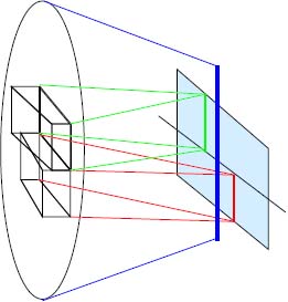
Figure 9.5. Principle of split-image focusing (stigmometer) as used in analog film cameras. The two right prisms are placed top to bottom, and use a very small part of the viewfinder field (highly magnified in the diagram). They produce two images, which take different positions in the image produced by the rest of the optical pathway in the case of focal errors
In other cases, the distance is determined by measuring the travel time of an acoustic or an emitted and modulated infrared wave; the echo from the object is then detected and the angle is measured in order to determine the position of the target by triangulation. These two techniques are known as active telemetry, as a wave must be emitted. They are particularly useful in systems operating with very low lighting levels, but are less precise than split image focusing techniques. Using these systems, the value determined by the telemeter is often transmitted to a motor, which moves the lens assembly to the recommended distance. These systems were first used in film photography, and proved to be particularly useful in automatic capture systems (triggered by a particular event in a scene, whether in the context of surveillance, sports or nature photography).
With the development of solid-state sensors, telemeters became more or less universally used, and were subject to considerable improvements in terms of performance, to the point where user input was rarely required. In these cases, an electric motor is used in association with the lens assembly, and coupled with the telemeter. The focal technique is based on two different principles: first, attempting to obtain maximum contrast, and second (and most commonly), phase detection. However, ultrasound or infrared systems have also been used, often in a supporting role in addition to the main telemeter, to provide assistance in difficult situations (such as low lighting levels and reflecting or plain surfaces).
9.5.1. Maximum contrast detection
The basic idea behind this technique is to find the focal settings which give the highest level of detail in a portion of the image. Contrast telemetry, therefore, uses a small part of an image (chosen by the user, or fixed in the center of the field) and measures a function reflecting this quality. A second measurement is then carried out with a different focal distance. By comparing these measures, we see whether the focus should be adjusted further in this direction, or in the opposite direction. An optimum for the chosen function is obtained after a certain number of iterations. Three different functions may be used, which are all increasing functions of the level of detail in the image:
- – dynamics;
- – contrast;
- – variance.
Let i(x, y) be the clear image, presumed to be taken from a scene entirely located at a single distance p from the camera (see Figure 9.6).
When the image is not in focus, if the difference in relation to the precise focal plane is δ, the focal error is expressed in the approximation of the geometric optic by a pulsed response: circle(2ρ/ε) and the blurred image is given by:
where ε is obtained using formula [2.1].

Figure 9.6. Construction of a blurred image: point P is in the focal plane, and focuses on point P′. If we move in direction Q, by δ, the image is formed at Q′, at a distance δ′ = Γδ (where Γ is the longitudinal magnification, see equation [1.3]). The blur of Q′ in the image plane of P′ will be of diameter ε = Dδ′/p = δ′f/Np, where N is the aperture number of the lens assembly
The study domain for variations in i may be, for example, a line of 64 or 128 sensors, with a size of 1 pixel. Two perpendicular lines are often used together in order to determine contrast for horizontal or vertical structures, depending on the scene in question.
We immediately see that dynamic Δ(i′) must be lower than Δ(i), as i′max ≤ imax and i′min ≥ imin, due to the use of a low-pass filter which reduces the maximum and increases the minimum. Moreover, if d′ < d, then Δ(i′) < Δ(i), and the process will lead to correct focus, whatever the focal error, as Δ(i) is a decreasing function of d.
Contrast measurement is rather more complex. Contrast evolves in the following way:
When we change the focus, the maximum luminosity is reduced by η and the minimum is increased by η′ (where η and η′ are positive): i′max = imax −η, i′min = imin + η. The contrast becomes:
and:
This is always positive, leading to the same conclusion obtained using dynamics; however, the command law obtained in this way is independent of the mean level of the image, something which does not occur when using dynamics.
For a variance measurement, v(i) = < (i − < i >)2 > = < i2 > − < i >2. The mean value < i > is hardly affected by the focal error due to the conservation of energy, whether the image is clear or blurred: < i >2 ~ < i′ >2. However, < i2 > is affected by the focal error. Using the Fourier space, let I be the Fourier transform of i(x, y) (I = F(i)). Parseval’s theorem tells us that < i2 >=< I2 >. In this case, from equation [9.1], we have:
with J1 the Bessel function of the first kind (equation [2.42]), and
Once again, the quantity decreases, and the process will finish at the point of optimum focus. The calculations involved when using variance are more substantial, but a greater number of measurements will be used before a decision is reached; this results in a better rendering of textures.
Using the maximum contrast method, two measurements are required in a reference point, to which the second measurement is compared in order to determine whether or not we have moved closer to the optimum. From these two values, we are able to determine the strategy to follow: continue moving in the same direction, or reverse the direction of movement.
9.5.2. Phase detection
Phase detection focus operates in a very similar way to split image focusing, comparing pairs of small images obtained using different optical pathways. However, the obtained images are not presented using a prism image, but rather using a beam splitter, extracting two smaller beams from the main beam and directing them toward two dedicated telemetry sensors for comparison (see Figure 9.7).

Figure 9.7. Simplified diagram of telemetric measurement in a digital reflex camera by phase detection. The semi-reflective zones T1 and T2 of the mirror direct light back toward photodetector bars, where signals from the edges of the target field are then analyzed
Phase matching occurs when the two images coincide exactly for a correctly calibrated position. The respective positions of the maximums on both sensors are used to deduce the sign and amplitude of the movement to apply, combined to give a single measurement. These systems, therefore, have the potential for faster operation, and are particularly useful when focusing on a moving object. However, phase detection is less precise than contrast detection, particularly for low apertures, as the angular difference between the beams is not sufficient for there to be a significant variation, notably as a function of the focal distance.
9.5.3. Focusing on multiple targets
Focusing is relatively easy when the target is a single object. However, different issues arise when several objects of interest are present in the same scene.
9.5.3.1. Simultaneous focus on two objects
The most conventional case of multiple focus involves focusing on two main objects. From Figure 9.6 and equations [2.8], we calculate the product q1q2, which, after a number of calculations, gives us the following equation:
This tells us that if ε is very low, then the focal distance required for optimal clarity of two points situated at distances q1 and q2 from the photographer is the geometric mean of the distances:
and not the arithmetic mean, (q1 + q2)/2, as we might think.
9.5.3.2. Average focus
Modern cameras include complex telemetry systems which determine the distance qi of a significant number of points in a field, typically from 5 to 20 (see Figure 9.8). The conversion of these measurements, {qi, i = 1,…, n}, into a single focal recommendation generally depends on the manufacturer, and targets are weighted differently depending on their position in the field.
There are a number of possible solutions to this problem.
One option is to select the distance p which minimizes the greatest blur from all of the targets. In this case, the calculation carried out in section 9.5.3.1 is applied to the nearest and furthest targets in the scene. Hence:
Another solution is to minimize the variance of the blur, so that we effectively take account of all measurements and not only the two extreme values. Using equation [2.8], the blur εi of a point qi can be expressed when focusing in p:
but the mean square error: ![]() does not allow precise expression of the value p which minimizes this error. In these conditions, we may use iterative resolutions or empirical formulas, for instance only taking account of objects in front of the central target, and only if they are close to the optical center.
does not allow precise expression of the value p which minimizes this error. In these conditions, we may use iterative resolutions or empirical formulas, for instance only taking account of objects in front of the central target, and only if they are close to the optical center.

Figure 9.8. Focal measurement zones, as they appear to the user in the viewfinder. By default, measurement is carried out along the two central perpendicular lines. Users may displace the active zone along any of the available horizontal or vertical lines, in order to focus on a site away from the center of the lens. In the case of automatic measurement across a wide field, the measurement taken from the center may be corrected to take account of the presence of contrasting targets in lateral zones
9.5.4. Telemeter configuration and geometry
For both types of distance measurement, the simplest sensors are small unidimensional bars of a few tens of pixels. In both modes, measurement is, therefore, dependent on there being sufficient contrast in the direction of the sensor. Contrast due to vertical lines is statistically more common in images, so a horizontal bar will be used (in cases with a single bar), placed in the center of the field.
Performance may be improved by the addition of other sensors, parallel or perpendicular to the first sensor, or even of cross-shaped sensors. Modern systems now use several tens of measurement points (see Figure 9.8). This raises questions considering the management of potentially different responses. Most systems prioritize the central sensor on principle, with other sensors used to accelerate the focusing process in cases of low contrast around the first sensor. Other strategies may also be used, as discussed in section 9.5.3: use of a weighted mean to take account of the position of objects around the central point, majority detection, compromise between extrema, hyperfocal detection, etc.
Most systems which go beyond the basic level allow users to select from a range of different options: concentrating on a specific object in the center of an image, a large area or the scene as a whole. Advanced systems allow users to select the exact position of the focal zone.
Phase-matching assemblies are well suited to use in reflex assemblies, as the beams can be derived using the field mirror (see Figure 9.7). They are harder to integrate into hybrid or compact cameras, which, therefore, mostly use contrast measurement. Nevertheless, if focusing is carried out while the field mirror is in place, it becomes difficult to refocus in the context of burst photography of a mobile object.
If contrast measurement is carried out without beam splitting, pixels in the image plane need to be dedicated to this distance measurement. This means that the image for these pixels needs to be reconstructed using neighboring pixels (this does not have a noticeable negative effect on the image, as it only involves a few tens of pixels, from a total of several million). In the most up-to-date sensors, pixels are able to fulfill two functions successively, i.e. telemetry and imaging, and to switch between the two at a frequency of around 100 hertz. This idea has been generalized in certain sensors, where all pixels (2 by 2 or 4 by 4) are used in phase or contrast measurement.
9.5.5. Mechanics of the autofocus system
Focus commands are transmitted to the lens assembly. To ensure compatibility with manual adjustment, it acts via the intermediary of a helicoidal guide ring, used for both rotation and translation. Generally, all of the lenses in the assembly are shifted in a single movement. In more complex assemblies, it may act separately on the central system configuration, transmitting different movement instructions to subsets of lenses, divided into groups. In very large lens assemblies, the camera itself moves (as it is much lighter than the lens assembly), and the movement is, therefore, purely linear.
Movement is carried out by micromotors placed around the lenses. These motors constitute a specific form of piezoelectric motor, known as ultrasonic motors. Current models use lead zirconate titanate (PZT), a perovskite ceramic, to create progressive acoustic surface waves via a piezoelectric effect, leading to controlled dilation of very fine fins at a frequency of a few megahertzs. These fins, which are active in alternation, “catch” and move the rotor associated with the assembly, as shown in Figure 9.9. Note that these motors present a number of advantages: they allow very long driving periods, are bidirectional and do not create vibration, as the fins move by less than 1 μm at a time.

Figure 9.9. Operation of an ultrasonic autofocus motor. The terms “rotor” and “stator” are used by analogy with electric motors, despite the very different operating mode of acoustic wave motors. The movable ring (rotor) is the central structure. The stator is made up of three piezoelectric elements, which are either passive (shown in white) or active (dark) following a regular cycle, allowing the rotor to be gripped and moved in the course of a cycle. These elements dilate when active, producing gripping (stators 1 and 3) and movement (stator 2) effects. Carried by a progressive acoustic wave, the cycle repeats at very high rates without requiring any form of movement elsewhere than in the rotor
9.5.6. Autofocus in practice
Considerable progress has been made in the domain of focus systems in recent years, both for contrast and phase detection methods. With the assistance of ultra-fast motors, very precise focus can now be achieved in very short periods, i.e. a fraction of a second. This progress is due to the development of focusing strategies and the multiplication of measurement points, helping to remove ambiguity in difficult cases; further advances have been made due to improvements in lens assemblies, which are now better suited to this type of automation (with fewer lenses and lighter lens weights).
Recent developments have included the possibility of connecting autofocus to a mobile object, i.e. tracking a target over time, and the possibility of triggering capture when an object reaches a predefined position.
However, certain situations are problematic for autofocus:
- – highly uniform zones: cloudless sky, water surfaces, bare walls, fog, etc.;
- – zones with moving reflections (waves, mirrors, etc.);
- – zones with close repeating structures;
- – zones of very fast movement (humming bird or insect wings, turning machines, etc.);
- – very dark zones.
In practice, a situation known as “pumping” is relatively widespread in autofocus systems. This occurs when the focus switches continually between two relatively distant positions without finding an optimal position.
Note that while camera manufacturers aim to create systems with the best possible focus and the greatest depth of field, photographers may have different requirements. Excessively sharp focus in a portrait or on a flower, for example, may highlight details which the photographer may wish to conceal. Similarly, excessive depth of field can impair artistic composition, highlighting secondary elements that we would prefer to leave in the background. Photographers, therefore, need to modify the optical aperture or make use of movement in order to focus the observer’s attention on the desired elements (see Figure 9.10, left).
As the quality of blurring is important, photographers use specific forms of diaphragm to produce harmonious graduation. In this case, diaphragms with multiple plates, which are almost circular, are better than diaphragms with five or six plates for the creation of soft blurring, which is not too sudden or angular. Different shapes of diaphragm may also be used, such as right angles and stars, in which case source points in the background appear through the blur in the precise shape of the diaphragm image (creating bokeh). Bokeh is generally produced against dark backgrounds (distant light sources at night, reflected sunlight; see Figure 9.10, right). Note that catadioptric lens assemblies9, in which the optical elements are bent using ring-shaped mirrors, produce a very distinctive form of ring-shaped bokeh.

Figure 9.10. Blurring is an important aspect of the esthetic properties of a photograph. Left: spatial discrimination of objects exclusively due to focus. The choice of a suitable diaphragm is essential in softening contours. Right: the lights in the background are modulated using the optical aperture, giving a classic bokeh effect. For a color version of this figure, see www.iste.co.uk/maitre/pixel.zip
9.6. Stabilization
All modern cameras include an image stabilization system, used to limit the effects of user movement in long shots taken without a tripod.
Traditionally, in hand-held photography, without stabilization, and using full-format cameras (i.e. with 24 mm × 36 mm sensors)10, in order to avoid the risk of movement, the exposure speed should generally not be below 1/f (f expressed in millimeters, giving an exposure speed in seconds). This is known as the inverse focal length rule. Thus, a photograph taken with a 50 mm objective may be taken in up to 1/50 s, while a photo taken with a 300 mm distance lens should be exposed for 3/1000 s at most11.
Stabilization reduces the need to adhere to this rule.
Lens assembly stabilization is carried out using a motion sensor. The signals produced by these sensors are sent to the processor, which identifies the most suitable correction to apply, by projecting the ideal compensation onto the mobile elements available for stabilization, acting either on the lens assembly (lens-based stabilization) or on the sensor itself (body-based stabilization).
9.6.1. Motion sensors
Two types of sensors may be used in cameras: mechanical sensors, made up of accelerometers and gyrometers, and optical sensors, which analyze the image flow over time. Linear accelerometers are simple and lightweight components, traditionally composed of flyweights which create an electrical current by a variety of effects (Hall, piezoelectric or piezoresistive). These components have now been highly miniaturized and integrated into micro-electro-mechanical systems (MEMS) [IEE 14]. Linear accelerometers obtained using photolithography are often designed as two very fine combs, made of pure silicon, which interlock face-to-face. During acceleration, the capacitance between the combs changes, providing the measurement (see Figure 9.11). Gyrometers, which identify angular rotations, generally measure disturbances to the movement of a rotating or vibrating body (measuring the Coriolis force, which leads to a precession of movement around the rotation axis). The physical effects used in MEMS structures are very fine, and principally result from various types of waves resonating in piezoelectric cavities, of ring, disk or bell form; unlike earlier mechanisms, these techniques do not require rotation of the sensor.
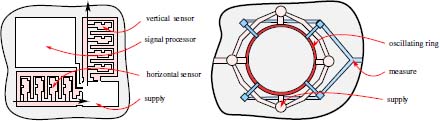
Figure 9.11. Left: two linear accelerometers using MEMS technology, made from interlinking combs, integrated into the same housing. These devices are used to determine translation movement in the plane of the host circuit. Right: a gyroscope, consisting of a vibrating ring (red, center). A circuit (shown in pink) is used to maintain vibration of the ring, while another circuit (in blue) measures deformation of the ring due to rotational movement. These two types of captors are produced from raw silicon. For a color version of this figure, see www.iste.co.uk/maitre/pixel.zip
Two accelerometers need to be used in a camera in order to determine the level of translation in the image plane. A third, the length of the optical axis, is rarely solicited. The three gyrometers are often integrated into a single circuit. The combination of the accelerometer and gyrometer gives us an inertial platform. Magnetometers may also be used to determine movement in absolute terms. The influence of the guidance system and games markets, the car manufacturing industry and telecommunications has led to miniaturization of these systems and a considerable reduction in cost. However, many cameras only use linear displacement accelerometers. Measurements obtained using mechanical sensors have the advantage of insensitivity to the movement of objects in a scene, unlike optical sensors. Mechanical sensors also have a much higher capacity than optical sensors to measure very large movements. If movement sensors are used in an open loop, the measured movement value must be used to deduce the effect to apply to the image sensor or correcting lens in order to correct the effects of this movement on the image. To do this, we need to take account of information concerning optical settings (focal length and distance). For this reason, it may be useful to use a closed loop mode, locking the mobile pieces into the control loop; however, this method requires the use of a mechanism within the image to measure stability. In practice, this mechanism carries out a function very similar to one required by the sensor, taken from the image, which will be discussed in the following section.
Optical flux analyzers implement similar functions and mechanisms to those used for autofocus (in some cases, these are one and the same). Measurements of the spatio-temporal gradient are determined across the whole field, at very close sampling times, using block-matching techniques. These operations will be discussed further in section 10.1.6. The denser the measurement field, the higher the precision of calculation, and the higher the charge on the calculator. Calculations may be accelerated in tracking mode by maintaining parameters using predictive models (ARMA models, Kalman filters or particle filters), either directly using measurements at each individual point, or on the basis of global models obtained by analyzing all of the points as a whole:
- – if the speed field is relatively constant across the image, the movement is a bi-dimensional translation; this is the first fault to be corrected, and is generally the most significant error;
- – if the speed field presents rotational symmetry along with linear and radial growth, this demonstrates the presence of rotation around the optical axis (see Figure 9.12);
- – if the symmetry of the speed field is axial, we have rotational movement in a downward or upward direction (tilt).
Optical sensors express the movement detected in an image in terms directly compatible with the compensation to apply to the image. These calculations are made considerably easier by the presence of the DSP and by the use of multiple parallel processing lines.
Note that different movement measurements are obtained from optical and mechanical motion sensors:
- – if the whole scene is scrolling, an optical sensor will integrate the movement of the scene into that of the camera, something which the user may not necessarily wish to happen;
- – if a camera is accelerating in a moving vehicle, an accelerometer will combine the movement of the camera with that of the camera, which, once again, may be contrary to the wishes of the photographer.
To take account of this type of major movement by carriers, certain manufacturers have introduced a “drive” mode which specifically compensates for significant, uniform movement. This mode should not be confused with stabilized mode, and will not be discussed in detail here.
Note that gyrometers (which provide tiny temporal variations in the angular orientation) should not be confused with gyroscopes (which measure the orientation of the sensor in relation to the Earth: North-South, East-West, azimuth-nadir), which are included in certain high-end products and provide additional details regarding the position of a scene, adding the three orientation angles to the GPS coordinates (the full equations involved in this stabilization are obtained using the calibration equations [2.47]).
9.6.2. Compensating for movement
Once the corrections needed to compensate for movement have been identified, we need to apply these changes to the actuators involved in compensation. As we have seen, two options exist in these cases: moving the sensor, or moving the lens.
Body-based stabilization is an economical solution, as it allows the use of any lens assembly, even those not adapted for stabilization. Furthermore, the sensor is lightweight and easy to move, giving it the ability to respond rapidly to a stabilization order. The actuator command laws are deduced directly from the measurements obtained by the sensor, a fact which simplifies the calculations required and reduces compensation errors. For motion compensation purposes, the sensor is placed onto a mobile unit, which moves across ball bearings using a piezoelectric motor (similar to those discussed in section 9.5) or a coil/electromagnet assembly. In reflex cameras, antidust systems may also be used for stabilization, as they apply vibrations to the sensor in the same way as the stabilization. However, body-(or sensor-)based stabilization does have its drawbacks. First, it may lead to excessively large sensor movements in cameras with a long focal length (several tens of pixels). Next, to compensate for complex errors (for example, dips and raises), complex movements are required, while the sensor must be kept in a very specific position in order to ensure capture quality.

Figure 9.12. Top: stabilization in response to three movements: translation, x0 and y0 (left) and rotation γ around the optical axis (right). Bottom: additional stabilization, rotating around the horizontal axis: dipped (α) and raised (β), giving a total of five parameters to control (the notation used is taken from equations [2.47]–[2.49])
If we act instead on optical elements, an additional connection must be established between the body and the lens assembly, and the camera in question can only be used with lens assemblies designed to be compatible with the specific stabilizer model. To limit the weight of the mobile element, a small group of lenses is generally moved, selected to be as light as possible. For assemblies with a long focal length, acting on the lens requires smaller movements than those required when moving the sensor. Crossed electromagnets are often used as actuators in order to generate this compensation movement. The compensation law requires us to take account of the image formation sequence as a whole (requiring calculations using the setting parameters). On a more positive note, lens position is less critical than that of the sensor in body-based stabilization. Note that in this case, it is not possible to compensate for rotation around the optical axis, but it is relatively easy to correct rotation around the horizontal axis. Unlike body-based stabilization, lens-based stabilization is beneficial for all camera functions: focus, light measurement, framing, etc. This is particularly beneficial when using long focal lengths.
Nowadays, the two types of stabilization system offer relatively similar performance levels. Note that lens-based stabilization was developed very early on for use in high-end film cameras12. It is also used in binoculars, microscopes and telescopes, and therefore has a longer and more impressive pedigree. Body-based stabilization was developed for solid-state sensors, at a time when stabilized lenses were already available. This solution is becoming increasingly popular. Newer propositions include hybrid systems, combining the two stabilization modes using a strategy determined by individual manufacturers; in these approaches, sensor stabilization is generally used to compensate for vibrations, which require rapid response times and significant lens movement [ATK 08]. This form of hybrid stabilization could become the dominant technology in the field if the command laws were to be made public, allowing interoperability between products.
It is also important to consider the types of movement compensated by an image stabilizer. First, motion compensation is particularly suited to correcting errors resulting from hand-held photography, i.e. erratic movements, generally vibrations, of low amplitude, affecting the sensor at an approximate rate of under 50 Hz. The main components of this motion are generally horizontal and vertical translations. Entry-level cameras and cell phones generally include stabilization functions for this type of error, and are also often able to compensate for rotation around the target axis. These three correction types are included in the three-axis stabilization approach (see Figure 9.12).
More advanced systems offer five-axis stabilization, which compensates for upward and downward tilt in addition to the three other movement types. Note that the distortions resulting from tilt (unlike those due to translation and rotation) are not isometric, and result in spatially variable blurring, which are difficult to correct by deconvolution13.
Stabilization is remarkably effective in terms of allowing longer exposure times. It is usually expressed in diaphragms, and can reach four or five diaphragms in the best cases; this results in a reduction of minimum exposure speed by a factor of 16 or 32. It is now possible to take photographs of fixed objects with exposure times of several tenths of a second without using a tripod, something which was barely possible 20 years ago. A more appropriate form of the inverse focal length rule, discussed at the beginning of this section, for modern apparatus would be 10 times the inverse of the focal length.
The possibility for confusion between movement in a scene and movement of the camera, mentioned above, requires further consideration. For this reason, it is best to avoid using the stabilizer if the camera is placed on a tripod14. Another, related, issue is the high-power consumption of a stabilized camera, as stabilization is active from the moment the camera is switched on, whether or not a photograph is being taken.
9.6.3. Video stabilization
The specific context of video photography, which concerns an increasing number of cameras, raises different issues to those involved in stabilizing fixed images. In this case, the main aim is not to reduce blurring during capture, but to keep the scene stable in spite of operator movements. Images must, therefore, be globally readjusted in relation to each other, while respecting the progressive movement of the frame imposed by the operator. Images are readjusted to each other using the motion detection methods (three or five axes) described earlier, but on the basis of 25 or 30 images per second, rather than the exposure times used in still photography. The available processing time is, therefore, longer, but the work required is more complex, as the movement accepted for an image n must be compatible with that accepted for images n − 1, n − 2, etc. The edge of fields is particularly problematic, as images are offset in relation to each other. The pixels from image n which have left the field due to parasitic movement, but should still be present as they were seen in n − 1 and n − 2, therefore, need to be temporally extrapolated. This specific treatment is relatively similar to that carried out by the P lines in MPEG coding (see Figure 8.9). These operations may be carried out in real time in the camera using motion prediction. Offline treatment also remains possible, notably for replacing extrapolations with interpolations, and linear prediction with nonlocal approaches, which are costly in terms of processing time but are highly effective.
Another problem affecting video images taken with a CMOS sensor with an electronic sensor resides in the fact that the capture instant is not the same at the top and bottom of the image, as the CMOS dumping process is sequential (see section 3.2.3 and the discussion in section 9.4). If the camera is subject to non-vertical movement, then vertical lines will be distorted. This effect should also be corrected during the readjustment process.
9.7. Additions to the lens assembly: supplementary lenses and filters
Let us now consider the accessories used to improve or modify the properties of the lens assembly, as discussed in Chapter 2. We will begin by discussing additional lenses, used to modify the focal distance of the objective, followed by filters, which affect the photometry of the image. To conclude this section, we will then consider polarizers. All of these filters are placed in front of the lens assembly (between the assembly and the object being photographed), with rare exceptions being placed between the lens assembly and the body of the camera.
9.7.1. Focal length adjustment
9.7.1.1. Close-up lenses
Photographers regularly make use of additional lenses, fixed onto the lens assemblies, known as close-up filters or close-up lenses. These often consist of a single convergent lens, or an achromatic doublet, and always take the form of a lightweight element which is added to the objective in the same way as a filter. Close-up lenses operate by bringing the infinite plane in to a short distance from the camera, in order to allow more significant magnification than those obtained with the lens assembly alone. Used for excessive zooming, close-up lenses can cause aberrations, limiting their usefulness. They are most effective when used with long focal length assemblies, increasing the focal length still further. For this reason, close-up lenses are often particularly useful in outdoor photography.
Close-up lenses are defined by their optical power, expressed in diopters15. Most close-up lenses have a power of between 1 δ and 10 δ.
9.7.1.2. Teleconverters
A teleconverter is a secondary lens assembly which is placed between the camera body and the lens, and fulfills the same role as a close-up lens. 2 × teleconverters are the most widespread. 3 × teleconverters also exist, alongside lower multipliers, for example 1.3 and 1.5. Teleconverters are relatively complex optical systems (up to 10 lenses) and are relatively large (particularly in comparison with close-up lenses), with a thickness of several centimeters. They operate in the same way as a divergent lens. 2 × teleconverters generally produce fewer aberrations than close-up lenses, and for this reason they are often used for photographs taken at short or very short distances, where close-up lenses are often unsuitable.
As with close-up lenses, teleconverters magnify the core of an image in the sensor, reducing the energy received by the sensor; higher exposure settings are, therefore, required (a 2 × teleconverter requires an exposure time 4 times that of the lens assembly alone for the same aperture settings).
9.7.1.3. Focal length!dividers
A system symmetrical to the one described above may be used to replace a divergent assembly with a convergent assembly, placed between the lens assembly and the camera body, in order to reduce the size of the image. The advantages of this technique are not immediately apparent, but it can prove beneficial. These devices constitute a second type of teleconverter, sometimes referred to as a focal length divider (in contrast to the multipliers discussed above)16. This type of teleconverter produces a smaller image of the subject and covers a wider area of the scene. The received energy is, therefore, concentrated, allowing a reduction in exposure time (or lens closure; see Figure 9.13). These elements are sometimes presented as a means of increasing the aperture of the lens assembly (this is not true, and not physically possible, as it would require the collection of light from outside of the diaphragm). However, as they reduce the focal distance, for a constant aperture, they produce an effect identical to that obtained by increasing the aperture number, as N = f/D.
Focal length dividers were first introduced for use with digital cameras; as we clearly see from Figure 9.13, they can only work if the lens assembly is overdimensioned in relation to the sensor, otherwise an unacceptable level of vignetting is produced. Moreover, they can only be used if the flange focal distance (FFD, the distance between the sensor and the last lens) can be significantly reduced, as the equivalent focal distance is shorter. This is very hard to do using a reflex camera due to the presence of the mirror tilting mechanism. Focal length dividers are, therefore, only used in non-reflex cameras with changeable lens assemblies [CAL 12].

Figure 9.13. Effect of a focal length divider (lens booster). Left: the field covered by a lens assembly for use with a 24 × 36 sensor (the white circle), shown for three different formats of commercial sensor: 24 × 36, APS-C and 4/3. Right: the same lens assembly, with the addition of a focal length divider. The 24 × 36 format is now subject to high levels of vignetting. The two others are still in full light and benefit from the effects of focal length reduction. In practice, focal length dividers are used in this final configuration
9.7.1.4. Extension tubes and bellows
Extension tubes are optically passive elements, placed between the camera body and the objective, which are used to increase the flange. These elements are essential in macrophotography, allowing increasingly strong enlargements G as the length increases, following relationship [1.3]: G = −(f + p′)/f. In order to conserve camera settings, these tubes also need to be able to transmit sensor measurements to the actuators, making them complex and costly.
Camera bellows function using the same principle. One of the rings is placed on a mobile unit, and the length of the element can then be adjusted to suit the desired enlargement size. Tubes generally have a length of a few centimeters, but bellows can cover tens of centimeters, allowing significant levels of enlargement. However, this results in a very shallow depth of field and requires long exposure times. Both extension tubes and bellows are generally used with mid- and short-focal length assemblies with high apertures.
Other specific types of ring include inversion rings, which allow lens assemblies to be mounted in the wrong direction: in these cases, the input lens is situated nearest the sensor, while the original fixture mounting is closest to the object. For mid-focal length lens assemblies (between 30 and 85 mm), this creates very significant enlargements (as the nodal plane of the sensor is pushed back), comparable to those obtained using long extension tubes. Another type of ring allows lens assemblies to be joined together in a top-to-bottom configuration, producing enlargements of 20–50; however, this is accompanied by a significant loss of light (see Figure 9.14).

Figure 9.14. Three camera lens assemblies: left, standard assembly, allowing focal lengths from tens of centimeters to infinity; center: inverse assembly, producing significant enlargements for nearby objects; right: two assemblies, placed top to bottom in order to produce extremely high enlargement levels
9.7.2. Infra-red filters
We will only provide a brief description of infra-red (IR) filters here. These filters are generally placed on the input end of the lens assembly. They fulfill two key roles:
- – as their name indicates, they suppress IR radiation (with a wave length greater than approximately 780 nm), to which the silicon used in sensors is particularly sensitive (see Figure 5.22); this radiation should not contribute to image formation, as it is not visible to the naked eye;
- – they protect the external face of the lens assembly from mechanical shock and dirt (water, dust, etc.).
This second property is often the most important, as modern solid-state sensors are well protected against IR radiation by treatments applied to the photodetector itself.
IR filters are made from either glass with a high level of absorption in the IR spectrum, or by applying thin layers of metallic oxides to thin glass plates, which act as interference filters. Interference filters have sharper cut-off lines, but their effectiveness is dependent on the angle of the rays, and they, therefore, offer very limited protection for lenses with a strongly-inclined capture angle (such as fisheye lenses).
Commercial filters differ in the sharpness of their cut-off limits, both above the red spectrum and below the blue spectrum. Excessively powerful treatments can result in a blue or, in the other direction, pink tinge in the resulting images.
Besides their performance in rejecting IR radiation, the quality of IR filters is determined by their mechanical hardness, their transparency across the visible spectrum and the antireflection treatment used.
Note that it is also possible to use filters to remove all light except for IR in order to create special effects, or to select thermal radiation in night-time photography polluted by parasitic noise. As we have seen, this is only possible if the IR filter on the sensor is also removed.
9.7.3. Attenuation filters
Neutral filters attenuate the beam following a wavelength law which is generally uniform17. These filters are characterized by their optical density, i.e. the inverse of the common logarithm of their transparency. Thus, a filter with a density of OD = 1 attenuates light with a ratio of 10, which may be offset either by multiplying the diameter of the diaphragm by around 3.16, or by multiplying the exposure time by 10. Filters are available with a density of between 1 and 10. Attenuations are also sometimes described using the number of equivalent diaphragms, ND. This is the base 2 logarithm of the OD : ND = OD/log10(2) = 3.32OD.
The interest of using a neutral filter, which reduces the amount of light in an image, lies first in the possibility of photographing scenes with very high luminosity, such as those encountered in industrial or scientific photography (eclipses, volcanoes, furnaces, etc.). It also allows more “everyday” photographs to be taken using very long exposure times, allowing the creation of special effects, for example for a water course, the sea or a moving crowd. Finally, neutral filters are very useful when using wide lens apertures in scenes where we wish to reduce the depth of field.
Certain neutral filters may only cover half of the optical field, in order to adapt to contrasting lighting conditions; in this way, the sky and ground are treated in different ways. This local treatment may also affect spectral content, for example increasing the levels of blue in the sky.
These filters are made using glass plates or gels. They are screwed onto the lens assembly, or held in place by a filter holder structure. Note that the use of two mobile polarizers, which can be moved in relation to each other, or, better, two polarizers followed by a quarter wave plate, constitutes an excellent variable attenuator, for reasons which will be explained in the following section.
Note that high attenuator densities render the photosensitive cells, which determine exposure time, and autofocus systems less efficient.
9.7.4. Polarizing filters
Polarizing filters are often used to produce specific effects on an image, for example damping reflections, reinforcing contrasts and tints, or modifying the appearance of certain shiny objects.
These effects can be explained by physical phenomena relating to electromagnetic propagation.
9.7.4.1. Physical considerations
Equation [1.1], as seen at the beginning of this book
is written in a specific scalar form for use in optics, which only takes account of the amplitude of the electromagnetic field, without considering its orientation. A fuller, vectorial form provides a more complete description of the electromagnetic field, describing the two components of the field in a plane normal to the propagation vector k. In air, a homogeneous medium (and the medium for almost all photographs), the electromagnetic field consists of two vectors, the electric field E and the magnetic field B, which are in phase but orthogonal to each other, in a plane orthogonal to the propagation vector k, and tangential to the wave front. Choosing a fixed direction for this plane, E can be subjected to unique decomposition, for example into two components E|| and E⊥.
The relationship between E|| and E⊥ defines the polarization of the wave:
- – if the two components are unrelated, the light is not polarized;
- – if E|| and E⊥ are in phase
 , the polarization is said to be linear. In one direction, the component of E, vectorial sum of E|| and E⊥, is maximized; in an orthogonal direction, its component is always null;
 - – if E|| and E⊥ are dephased, the vector E, sum of these two components, turns around vector k. In this case, the polarization is said to be elliptical. If ||E|||| = ||E⊥||, we have circular polarization, and the wave will have the same energy whatever the direction used for analysis.
9.7.4.1.1. Changing polarization:
It is possible to move from a non-polarized or elliptically polarized wave to a linear polarized wave by using a polarizing filter, reducing the energy of the incident beam by a factor of around 2. A quarter wave plate is used to change a linear polarized wave to a circularly polarized wave. To transform a polarized wave (of any type) into a non-polarized wave, a random diffuser is placed in the optical pathway [PER 94].
Polarizing filters are generally made up of microstructured materials, such as Polaroid, which will be described later. Waves which are polarized in the direction of alignment are stopped, while those which are perpendicular to the direction of alignment are transmitted with almost no attenuation.
Quarter wave plates are made of a birefringent material, presenting two different indices dependent on the direction of polarization. Placed at 45° to a polarized wave, they decompose this wave into two orthogonal components18.
Natural light is generally not polarized. However, the state of polarization can vary in relation to the medium through which it travels [FLE 62], as we will see below.
In photographic terms, non-polarized light and circularly-polarized light are indiscernible, and the terms are often used synonymously even in specialist publications.
9.7.4.1.2. Polarization and photography
If the incident light received by the sensor is selected on the basis of polarization, it is possible to increase or dampen contrast in an image. The simplest approach consists of placing a linear polarizer in front of the lens assembly. If the whole of the scene is made of non-polarized light, then the resulting image will only be damped (theoretically by a factor of 2, but sometimes slightly more in practice, as the glass used to support the filters absorb and reflect a small quantity of light in addition to the effects of the polarizer). Given a sufficiently long exposure time, however, the image will be identical to the original, whatever the direction of the polarizer. This is also true in cases of circularly-polarized light, although this situation rarely occurs in natural conditions.
If the light is polarized for certain objects, the resulting intensity will vary based on the direction of the filter, which may be placed parallel or perpendicular to the direction of polarization, from complete removal to full lighting. In the perpendicular case, all of the light from the polarized objects will be transmitted, unlike that of the rest of the scene, and these objects will be highlighted, appearing twice as luminous as the scene itself. In the parallel case, light from the polarized objects will be completely blocked, and these objects will appear dark. For an angle α between the filter and the incident polarization, the resulting intensity ||Es|| is obtained as a function of the incident intensity ||Ee|| using:
This is Malus’ law [PER 94]. It is, therefore, possible to highlight or conceal certain zones of an image simply by turning the polarizer around the optical axis. To identify the zones concerned by this treatment, we need to consider the causes of polarization.
9.7.4.2. Nature and polarization
9.7.4.2.1. Specular reflection
The Snell–Descartes law [JAC 62] states that if a wave is reflected from a dielectric of index n at an angle of i in relation to the normal plane, the reflected wave follows an angle which is symmetrical to i in relation to this normal plane. Polarization which is parallel to the reflecting surface reflects with an amplitude of E|| (see Figure 9.15, left) and the orthogonal component reflects with an amplitude E⊥. For a non-polarized incident wave, ratio R varies as a function of angle i following the relationship:

This function is illustrated in Figure 9.15, right. We see that the ratio cancels out for an angle at which the emergent wave is fully polarized. This is Brewster’s angle. At normal incidence (i = 0) and grazing incidence (i = 90°, but this is not particularly interesting, as both waves are null in this case) the wave remains circular, with equal components. In natural imaging, it is very hard to remove all reflection; however, it is possible to achieve a significant reduction (see Figure 9.16).
9.7.4.2.2. Microstructured materials
Light, like all electromagnetic waves, reacts in a very specific way to periodic structures with a period close to that of the wavelength, and its response is strongly linked to polarization. In the field of optics, these dimensions are less than 1 μm, making them barely perceptible for observers; however, the polarization effects are still significant. This effect concerns materials such as insect exoskeletons, hummingbird feathers, certain organic structures, pearlized surfaces and varnishes, and also certain biological tissue types (collagen fibers). These effects may apply to surfaces or volumes, and may affect certain specific wavelengths, but not others.

Figure 9.15. Left: reflection of a circularly-polarized wave on a plane and notation of emergent waves. Right: relationship between the energy of the emergent wave, polarized in parallel to the reflection plane, and that of the wave polarized in parallel to the plane, as a function of the angle of the incident wave and the normal of the reflection plane. The reflecting medium is a dielectric of index n, using three values of n. The incident wave is taken to be non-polarized. When the relationship cancels out, the emergent wave is completely polarized; this occurs at Brewster’s angle
Polaroid, invented by E.H. Land, is an artificial structured material made of a sheet of polyvinyl alcohol polymer, stretched in the manufacturing process in order to create aligned, linear chains of molecules. These chains are then treated with iodine to make them conduct, and take on strongly dichroic behavior: waves which are polarized in the direction of alignment are absorbed, while those polarized perpendicular to the chains are transmitted with almost no attenuation. Polaroid polarizers are widely used in photography.
9.7.4.2.3. Blue skies
The fact that the light emitted by a blue sky is polarized is generally explained by Rayleigh diffraction resulting from particles in the upper atmosphere ([BOR 70] p. 655). These particles are typically smaller than λ/10 in size. Solar radiation traversing these particles creates diffused radiation which is naturally polarized. Short wavelengths (i.e. blue) are diffused most (which gives the sky its blue color). Seen by an observer on the Earth, the degree of polarization π depends on the angle γ between the direction of the sun and the direction of the target point:

Figure 9.16. Photograph taken through a glass display case, showing the effects of a linear polarizer. Left: image taken without polarizer; right: image taken using a polarizer oriented so as to reduce the light reflected by the glass (Musée des Arts Premiers, Paris)
The degree of polarization is, therefore, null in the direction of the sun, and reaches a maximum at 90°. In physical terms, matters become much more complicated if we take account of multiple diffusions of the same ray, as short wavelengths are more susceptible to this type of diffusion, which removes polarization. The same effect can also result from diffusion by large particles (observed close to the horizon), which obey Mie diffraction laws; once again, this leads to greater desaturation of short wavelengths. The longest wavelengths (producing white light) may be absorbed by a carefully oriented polarizer, while blue wavelengths will represent the majority of those transmitted; however, these wavelengths remain rare, producing deep blue shades in the image.
9.7.4.2.4. Birefringent materials
Finally, polarization may also result from materials with rotary powers, which are said to be optically active. These materials naturally appear differently depending on the incident polarization. This is encountered in crystals (such as quartz) and certain liquids (such as benzene) ([FLE 62], Chapter 12).
9.7.4.3. Polarizer use
The use of linear polarizers to improve images is particularly simple. The best orientation is determined by direct observation of results on the monitor screen. However, this simple filter may have undesirable effects on the operation of a camera, as the sensors (both for autofocus and exposure) often operate by deriving part of the luminous flux traveling through the lens assembly using semi-reflective plates (see Figure 9.5). If the light is polarized, then the response from these captors will be wrong (as a direct function of Malus’ law, cited above). Many cameras also use an antialiasing filter (see Figure 3.10) which only operates correctly with non-polarized or circularly-polarized light.
The use of a more complex assembly for linear polarization is, therefore, recommended. This assembly consists of a linear polarizer followed by a quarter wave plate, placed at an angle of 45° in order to re-establish full polarization. These devices are generally known as circular polarizers. They only operate in one direction (with the linear polarizer in front of the quarter wave plate) and cannot be used in series for damping purposes, something which is possible with simple linear polarizers, unless the filter is mounted upside down; this is generally not possible due to the fixation mechanisms used.
In photography, polarizing filters are used to process natural scenes. In a scientific context, these filters may be used in a more complex way, by controlling both the polarization of the light source and the orientation of the analysis filter. This is known as polarimetric imaging. The process consists of a series of exposures, and by analyzing the images produced, it is possible to obtain a variety of information:
- – the nature of the surfaces under examination, which may retain or rotate the polarization (metallic or dielectric reflections) or destroy the polarization (rough surfaces, absorbent or diffusing materials);
- – the orientation of surfaces relative to the retention or rotation of polarization.

Figure 9.17. Polarization using a linear polarizer followed by a quarter wave plate, allowing reconstruction of a non-polarized wave (C), from the incident light (A) of which only a linearly polarized component (B) has been transmitted by the linear polarizer. Assemblies of this type allow the optical components of the camera to function correctly, while removing one of the polarizations of the scene. The two plates should be moved as a single unit during rotations in order to find the angle of absorption
9.7.5. Chromatic filters
In this section, we will consider filters which modify the overall appearance of a scene, and not chromatic selection filters, which are placed over the sensor and were examined in section 5.4.
The most important filters of this type are color correction filters. We have already seen (Chapter 4) the way in which the color temperature of a scene is defined, particularly in the case of artificial lighting. The spectral content of this light may be different from that desired for a photograph, either because the light is too cold (too much blue), or too warm (too much red). This problem may be corrected by the introduction of a filter, which acts on the incident spectrum so that it meets the photographer’s requirements.
Let Ti be the color temperature of the incident source and To the desired color temperature. Wien’s formula (which is a very good approximation of Planck’s law for the temperatures ordinarily used in photography) provides an expression of the spectral luminance corresponding to these values (equation [4.17]):
where h is Planck’s constant, c is the speed of light and k is the Boltzmann constant.
The filter used to pass from Ti to To thus has a spectral transmittance T(λ, Ti, To):
where α is an arbitrary constant which ensures that ![]() is less than 1 across the whole spectrum. Filters are often described using their optical density (the normal log of their transmittance):
is less than 1 across the whole spectrum. Filters are often described using their optical density (the normal log of their transmittance): ![]() . Hence:
. Hence:
The spectral density of the filter is therefore linear in terms of the wave number σ = 1/λ, and is a function of the inverse of the temperature [BUK 12]. Each temperature is associated with a source characteristic, expressed in reciprocal megaKelvins19, equal to 106/T, and the filter is defined by its value in reciprocal megaKelvins. Thus, a 133 reciprocal megaKelvin filter converts light from an incandescent lamp (Ti = 3 000 K, i.e. 133 MK−1) to the equivalent of lightly softened sunlight (To = 5 000 K, i.e. 200 MK−1).
9.7.6. Colored filters
In addition to temperature correction filters, colored filters are often widely used, essentially in the context of black and white photography, in order to create specific effects by heightening certain tints. They are often used for this purpose by professional photographers. Notable examples include:
- – red filters: generally used for dramatic or “fantasy” effects, absorbing blues and greens. They can be used to increase contrast in clouds, waves or whirlpools, for example. They are also essential for daytime IR photography;
- – orange filters: often used for portraits, as they can produce a range of flesh tones, eliminating zones of redness. They are also useful when photographing natural environments with a high mineral content, such as deserts and mountains;
- – yellow filters are used for landscape photography in cases of low light, as they harden blue tones and increase contrast;
- – green filters are generally used to highlight vegetation, and are suitable for use in landscape photography. They also give a tanned appearance to flesh tones.
9.7.7. Special effect filters
We will not go into detail concerning the wide range of special effect filters available here; we will simply describe a number of broad categories.
Soft filters have an attenuating effect on microcontrast. They are often made from a very fine diffusing structure (microbubbles in glass, very fine matte effects, etc.), used to reduce the level of fine detail in a scene, generally in order to reinforce a steamy or misty effect. These filters are widely used in portrait and nude photography, where they help to reduce the appearance of skin imperfections; they may also be used in landscape photography, and are widely used in advertising. Note that soft filters do not necessarily have to cover the whole field; they may only cover half of the space, the center of the field or only the edges of the field. Another type of soft filter produces a graduated effect across the field.
Directional filters consist of very fine, transparent structures, oriented either in a linear manner (one or two dimensions, crossed or in a star configuration) or radially. They contribute to a modification of the pulse response, and introduce a highly visible diffraction figure, resulting in the presence of stars or irisations (bokeh, as discussed in section 9.5). They are particularly useful when photographing scenes with strong light sources (e.g. in night photography).
Even more dramatic effects may be obtained using binary masks, which only allow light to pass through specific apertures: hearts, spirals, stars, clouds, silhouettes, etc. In mathematical terms, the effects of these masks may be analyzed using equations [2.35], [2.36] and [2.37], but they are only used in response to specific requirements, deforming the pulse response using a particular motif and distorting fine details in an image to give a particular esthetic effect.
Note that these filters act in exactly the same way as coded apertures, which will be discussed below.
9.8. Power cells
Modern cameras all require a source of current in order to power integrated electronic components. While these components themselves often have very limited requirements, the calculation power involved, along with a number of newer functions (stabilization, GPS, display, Internet connectivity, etc.), which are active even when a photograph is not being taken, is highly dependent on the power supply. Camera battery life, often expressed as a number of photographs, is not a particularly reliable or useful indicator. The practical battery life of a camera is often a major usage constraint in cases of intensive use, and a number of different options may be envisaged: use of mains power in a studio context, extension grips or, simply, carrying spare batteries.
Considerable changes are currently taking place in the domain of rechargeable batteries, and the field may be very different in the future from what we currently know [CHA 14]. However, for lightweight, portable devices such as cameras, the broad principles are unlikely to change, and are discussed below.
9.8.1. Batteries
The first cameras used either zinc-carbon (Zn-C) cells (zinc anode20, carbon cathode, with an ammonium or zinc chloride electrolyte) or, better, alkaline cells (Zn-MnO2: zinc anode, manganese dioxide cathode and potassium hydroxide electrolyte, KOH) which have a slightly longer life expectancy and a higher charge density. These cells, and their numerous variations, operate by a process of oxido-reduction, producing voltages of between 1.5 and 1.7 V. Taking the form of cylinders or disks, these cells are traditionally used in series and conditioned in parallelepipedic casings, giving a total voltage of up to 9 V. Batteries of this type are not generally rechargeable, but are cheap and widely available.
9.8.2. Rechargeable Ni-Cd batteries
For many years, nickel-cadmium (Ni-Cd) rechargeable batteries were used as an energy source in most cameras. This technology has been progressively replaced by Ni-MH (nickel-metal hydride) batteries, due to the toxicity of cadmium, a heavy metal which is now closely monitored and which was made illegal for mass-market usage in Europe in 2006.
Ni-Cd batteries use cadmium electrodes on one side and nickel oxide and hydroxide (NiOOH) electrodes on the other side. They deliver a relatively low voltage (1.2 V) and need to be placed in series or used with amplification methods to power camera processors. They present reasonable performance levels (energy-weight ratio of 40– 60 Wh/kg, charge/discharge yield of around 80%, a life expectancy of a few years, a cycle number of over 1,000 and a spontaneous discharge rate of around 20% per year).
Ni-Cd batteries are widely believed to be subject to “memory effects”, a generic term which covers two specific faults: first, a behavior which causes a battery, operating regularly between two precise charge and discharge points (as in the case of batteries integrated into satellites, which recharge during a specific phase of the circadian cycle) to lose the ability to function beyond this limit, and second, the formation of cadmium hydroxide crystals, reducing the usable surface of the anode, if the battery remains charged over a long period. In both cases, the result is the same: a significant loss in battery capacity. The first of these faults (that which may properly referred to as a memory effect) is still the subject of debate, and no irrefutable scientific explanation exists. The second fault, on the other hand, is known to be real. This fault does not produce a memory effect, but produces natural evolutions within the battery; furthermore, this change is reversible via the application of a suitable recharge cycle (reconditioning). However, most chargers are unable to carry out this process.
It is best to charge and discharge Ni-Cd batteries on a regular basis in order to avoid cadmium oxide crystallization.
Ni-MH (nickel-metal hydride) batteries were developed to replace cadmium at the anode once the ban became effective. These batteries use lanthane and nickel hydrides (of type LaNi5), in a potassium hydroxide electrolyte (KOH). The voltage of individual elements is the same as that obtained from a Ni-Cd battery, but the energy/weight ratio has increased to 100 Wh/kg. However, the discharge/charge ratio using this technology is only 66%, and the discharge rate is in excess of 30% per year.
Different manufacturers have issued very different recommendations concerning the best way of conserving Ni-MH batteries in order to attain the best possible capacity and life expectancy.
9.8.3. Lithium-ion batteries
The use of lithium for energy accumulation purposes is a relatively recent development in commercial terms (1991), although there was widespread awareness of its possibilities well before this date; this late development is due to the difficulties involved in conditioning these products.
Lithium-ion batteries operate via the exchange of lithium ions between a composite anode (for example, a carbon or graphite matrix) into which lithium is injected in a reversible manner, and a cathode made of a metallic oxide (such as cobalt oxide and manganese oxide) [YOS 09, HOR 14a]. Ions are exchanged within an aprotic solvent electrolyte, i.e. an electrolyte which will not release a H+ ion (lithium salt in an organic solvent). Rechargeable lithium batteries differ from their non-rechargeable cousins at the anode: disposable cells use metallic lithium directly, meaning that the cycle is irreversible.
Rechargeable Li-ion batteries offer a number of remarkable properties (see Figure 9.18). They provide high voltages of around 3.6 V, considerably higher to those obtained using different technologies; this voltage is directly compatible with integrated electronic circuits, and the batteries do not need to be placed in series. The energy/weight ratio is more than double that of Ni-Cd batteries, from 100 to 250 Wh/kg. The charge-discharge rate is greater than 80% and may even exceed 90%, and the spontaneous discharge rate is very low (less than 10% per year). Li-ion batteries are not subject to memory effects, removing the need for an initial learning cycle and for specific maintenance operations. Note, however, that for optimal storage, these batteries should be kept at around 40% charge, and at a temperature of around 15°C.
However, Li-ion batteries present a number of disadvantages; these may be overcome in part by changes to the basic components, but this often results in a loss in terms of other performance aspects. First, these batteries are expensive, around 50% dearer than their NI-Cd equivalents. This cost is unlikely to fall, due to the rarity of lithium and the scale of demand. Moreover, these components are chemically fragile, particularly at high temperatures, and precautions need to be taken while charging; this slows down the charging process, which follows a specific progression, starting with a constant current then progressively reducing this current until the battery is fully charged. The aging process for Li-ion batteries remains hard to control, and their lifecycle is too short (barely more than 500 charge/discharge cycles, and 2 – 4 years). They are subject to irreversible damage if the charge drops too low, and if the voltage falls below approximately 2 V. Li-ion batteries, therefore, need to be controlled by a specific circuit, which cuts off service before full discharge is reached. These circuits are often integrated into the battery casing itself, and are known as battery management systems (BMS). BMS are particularly important in the context of high-performance batteries. Finally, it should be noted that lithium is a combustible metal. Batteries may, therefore, catch fire or explode if the discharge current exceeds a certain level, for example due to an increase in temperature. The transportation of lithium batteries is subject to limitations, notably in the context of air transport; this constraint does not only apply to industrial contexts, as airlines also specify conditions for transporting rechargeable batteries in personal luggage21

Figure 9.18. The performances of rechargeable battery types used in photography are shown here using two variables: the energy/weight ratio and the energy/volume ratio, which constitutes an important criterion in miniaturized systems. Li-ion batteries currently offer the best performance from both perspectives (based on [HOR 14a])
Research into the improvement of lithium batteries is ongoing [HOR 14a], with a particular focus on cathode efficiency via the choice of active materials, including cobalt and nickel oxides; these new products are identified as LiCoO2, LiNiO2 or, more generally, LiMxNi−xO2, where M is a metal such as cobalt, magnesium, manganese and aluminum. Lithium-iron-phosphate (Li-FePO4) batteries, for example, have a longer life expectancy and are safer to use, but offer a lower energy/weight ratio. Other projects concern the replacement of the liquid phase electrolyte by a polymer electrolyte, in order to decrease the risks associated with housing rupture. These projects have yet to result in the creation of commercial products, but the term “lithium-polymer” (Li-Po) has already been used to designate batteries with a polymer-based housing. These batteries present interesting mechanical properties (notably the fact that they may take the form of very fine plates), but do not constitute significant progress from an energy perspective in relation to the classic Li-ion technology (they also have a relatively low life expectancy). Further work has been carried out with the aim of reducing charging time. Very good results have been obtained by replacing the graphite at the anode by nanoparticles of tin oxide, SnO2, which have no other effects on battery performance [ELA 14].
Finally, over a much longer term, researchers are considering methods whereby current is produced by reduction of ambient oxygen at the cathode and oxidation of lithium at the cathode, creating a Li-air (lithium-air) battery. This technology potentially offers an energy/weight ratio 10 times higher than that of Li-ion cells; these solutions are intended for use in vehicles rather than cameras, but progress made in this increasingly significant sector is sure to have a knock-on effect in areas such as photography.