
4
Radiometry and Photometry
During the recording of a photograph, the light wave emitted by the scene is transformed into an image on film or on a photodetector. The image is the result of the transformation of the energy of the photons into electrical or chemical energy. The role of radiometry and photometry is to describe the parameters involved in this flux of photons.
Radiometry and photometry are two closely related sciences which have as a common subject of study the energy effects of light radiation. Therefore, they describe two complementary aspects:
- – radiometry is only concerned with the objective and physical aspects of radiation;
- – photometry considers the subjective, perceptual aspects of radiation and therefore the energy balances involved, such as the measurements of a reference observer, i.e. the human eye, along with its metrics.
Nevertheless, according to several authors, the term “photometry” is also associated with the physical aspects of radiation in the visual spectrum (radiometry being extended to areas not perceptible to humans). As a precaution, energy or objective photometry will be distinguished from visual or subjective photometry throughout this chapter [KOW 72, LEG 68, SMI 90].
In the field of photography, one is driven to maintain a close connection between these two aspects since a physical sensor is available. This is precisely related to the first aspect, but most often it is sought to assimilate it as closely as possible to criteria ensuing from the second.
4.1. Radiometry: physical parameters
4.1.1. Definitions
To photograph is to achieve the image of a point M on a sensor M′. In this chapter, we will consider the transfer of radiation energy between these points. We will first ignore all the optical elements which are used to form the image, and will consider that the photodetector is directly exposed to the radiation originating from the object M, as shown in Figure 4.1. Then, we will examine the role of the optical system. We will subsequently designate the point M as “source” since the light received by the sensors comes from there, but it may be a secondary source which merely reflects light from the primary light source (the Sun, a lamp, etc.). This aspect will also be considered.

Figure 4.1. Geometry in the neighborhood of point M of the surface imaged in a point M′ of the sensor
We assume the scene is fixed during the short exposure time δt. The energy E emitted by the source M in the direction of the detector is proportional to the exposure time. The spectral energy E(λ) is the share of this energy emitted in the small interval of wavelength ∂λ1.
4.1.1.1. Luminous flux
The luminous flux represented by Φ, expressed in watts, is defined as the power emitted by this source: Φ = E/δt, and the spectral luminous flux (expressed in watts per meter (SI unit), or more commonly in watt by micrometer2) is denoted by Φ(λ).
4.1.1.2. Radiant intensity
The radiant intensity of the source is by definition the flux per solid angle surrounding an observation direction θ. It is expressed in watt/steradian and is, therefore:
The spectral intensity is defined similarly:
In the calculation of intensity, the source is considered as a whole. The distribution of the emission on its surface is not distinguished.
4.1.1.3. Irradiance
The irradiance3 of an object is defined as the intensity per area unit in the direction of observation. It is, therefore, the luminous flux emitted by the elementary surface ∂s of the source in a small solid angle ∂ω around the direction θ (Figure 4.1):
The dependence of irradiance with respect to the direction of observation θ is a property of the material. If ![]() (θ) is not depending on θ, it is said that the source is Lambertian; Lambertian emitters are good approximations for a large number of matte or rough surfaces in nature photography. Conversely to the Lambertian surfaces, there are monodirectional sources such as lasers and specular surfaces that only reflect in a single direction.
(θ) is not depending on θ, it is said that the source is Lambertian; Lambertian emitters are good approximations for a large number of matte or rough surfaces in nature photography. Conversely to the Lambertian surfaces, there are monodirectional sources such as lasers and specular surfaces that only reflect in a single direction.
Similarly, the spectral irradiance can be defined from the spectral intensity ![]() :
:
Irradiance is expressed in watts per square meter, and steradian (W.m−2.st−1) and the spectral irradiance in W.m−3.st−1.
When M is a primary source, ![]() (θ) is known by its radiation pattern (also called far-field pattern). When M is a secondary source, it is defined using its reflectance (see section 4.1.4).
(θ) is known by its radiation pattern (also called far-field pattern). When M is a secondary source, it is defined using its reflectance (see section 4.1.4).

Figure 4.2. Geometry between the point M of the imaged object and the point M′ of the sensor for the calculation of the illumination. Surfaces ds and ds′ are carried on the one hand by the object, on the other hand by the sensor. The surfaces dσ and dσ′ are the straight sections of the two elementary beams, one such as the sensor sees the object, the other such as the object sees the camera
4.1.1.4. Radiance or exitance
Exitance4 ![]() (in watts/m2) characterizes the source and expresses the luminous flux emitted per unit area:
(in watts/m2) characterizes the source and expresses the luminous flux emitted per unit area:
and the spectral radiance:
For a Lambertian source (![]() independent of θ), as dω = 2π sin θdθ:
independent of θ), as dω = 2π sin θdθ:
4.1.1.5. Irradiance
Irradiance is the incident flux per unit area received by the sensor originating from the source. It depends both on the luminous intensity emitted by the source in the direction of the camera and on the orientation of the sensor, given ∂s′ the surface on the sensor around the point M′, described by the beam traveling from M and with a solid angle ∂ω. The surface ∂s′, including the normal, makes an angle θ′ with MM′ and receives the flux ∂2Φ emitted by the source. We have:
if r is the source sensor distance r = d(MM′).
By definition, the irradiance fraction of ∂s′ provided by the surface ∂s of the source on the sensor is given by:
4.1.1.6. Luminous exposure
It is the integral of the flux during the exposure time per area unit of the receiver. In practice, it is expressed by:
and is measured in joule/m2.
4.1.1.7. Total irradiance
M′, expressed in watt/m2, is given by the integral of all points of the object contributing to the pixel, that is to say the inverse image of the pixel:
Similarly, the spectral irradiance is equal to:
In photography, the observation distance of the various points of the object and the angle of the sensor are almost constant and thus, for small objects, we have:
4.1.2. Radiating objects: emissivity and source temperature
We have used here the equations of radiometry between an object and the sensor based on the knowledge of the energy E or the spectral energy E(λ), emitted by the object, assumed to be known. But how can these quantities be determined? We must consider two different situations: that where objects emit light and that where objects reflect it.
If most of the objects in a scene are passive and re-emit the light from a primary source, some radiate by themselves (flame, filament, etc.). These bodies whose behaviors are very varied prove generally difficult to characterize. This is achieved by reference to the black body defined in statistical thermodynamics as an ideal body which absorbs and re-emits any radiation to which it is exposed. The properties of the black body depend only on its temperature which thus dictates all its behavior. A black body at temperature T emits a spectral irradiance (expressed in W/m2 /sr/μm) that follows Planck’s law LEG 68, MAS 05:
where:
- – h is Planck’s constant: 6.626 × 10⁻³⁴ m2 /kg;
- – k is Boltzmann’s constant: 1.381 × 10⁻²³ m2kg/s2/K;
- – c is the speed of light: 299,800,000 m/s.
Irradiance is calculated independent of the angle θ: the black body is Lambertian. In the SI system (see Figure 4.3), Planck’s law is written as:

Figure 4.3. Emission of the black body temperature (in steps of 500 K) for wavelengths ranging from the ultraviolet to near-infrared, on the left as a function of wavelengths, and on the right as a function of frequencies (the visible spectrum lies between 700 (purple) and 400 (red) THz)
The total irradiance of the black body ![]() cn in the visible spectrum is, therefore:
cn in the visible spectrum is, therefore:
In the visible spectrum and for a source of incandescence (T ∼ 3, 000 K), the exponent of the exponential of equation [4.14] acquires values in a range between 5 and 10. Ignoring the term –1 in the denominator of Planck’s law, thus obtaining Wien’s law, is often sufficient to solve problems in photography (Figure 4.4):
But, this approximation is often not sufficient in near-infrared.
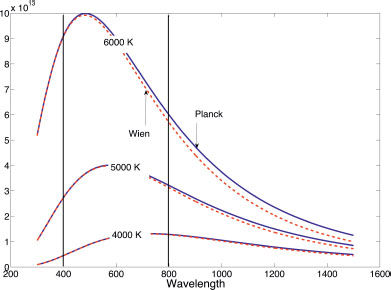
Figure 4.4. Wien’s (dashed line) and Planck’s (solid line) laws for the black body at temperatures of 4,000, 5,000 and 6,000 K. Radiations are virtually indistinguishable in the visible spectrum
From Planck’s law, the emittance of the black body is derived, by integration in the whole of the half-space and all wavelengths:
This is Stefan’s law, and σ, the Stefan constant, is 5.67 10−8 Wm−2K−4.
Another consequence of Planck’s law, the abscissa λm of the maximum irradiance curves, according to the wavelength, varies with the inverse function of the absolute temperature of the black body (formula referred to as Wien’s displacement law): λmT = 2, 898 × 10−6 mK.
4.1.2.1. Color temperature
For a given temperature T, Planck’s law (equation [4.14]) gives the maximal emittance that a body emitting light can achieve. In nature, where the emittance of a material is always less than that of the black body, it can be expressed by:
where ε(λ) is the spectral emissivity of the material, between 0 and 1.
If ε(λ) is not dependent of λ, it is said that the body is gray. It uniformly absorbs for all wavelengths a part of the radiation that the black body would reflect. A gray body is fully described by the temperature To of the corresponding black body and the value of ε: T = To.
If ε(λ) is dependent on λ, a search is launched among the black body curves for the curve that has the same wavelength behavior of the material being studied. If this behavior is reasonably similar, it is then said that the object behaves as the black body at temperature To. It yields that T ≠ To.To is called the color temperature of the object. How is the value of To found? Starting from equation [4.19], ε(λ) is expressed on the basis of 1/λ for all temperatures T using equations [4.17] and [4.19] and allowing the tracing of: log(ε(λ)) = f(1/λ). The most linear curve designates the most suitable temperature To because it has a slope proportional to 1/T – 1/To.
We will return to the transition from a color temperature to another using Wien’s formula in Chapter 9 where we describe the filters that can equip the objectives. This transition is based on filters which optical density varies inversely to the wavelength and proportionally to the difference between the inverses of the source temperatures (see section 9.7.5).
Nevertheless, this thermodynamic definition of color temperature is inconvenient because it requires a good knowledge of the sources, a condition hardly satisfied in practice. Therefore, in reality, empirical approaches are frequently used strongly based on spectral distribution hypotheses in the scene. We will encounter these approaches when we discuss white balance (section 5.3).
4.1.2.2. The tungsten case
Tungsten is used a lot for filaments of light bulbs because it has the highest melting point of all the metals (3,422 K). This allows us to create high brightness sources and a relatively high color temperature. The color temperature of tungsten is approximately 50 K higher than its real temperature in its operating range in the vicinity of 3,000 K. It should, however, be noted that the color temperature of tungsten remains low compared to that of daylight. To simulate daylight, this color temperature is altered by inserting a colored filter in front of the source (or the sensor), as we will see in section 9.7.5.
The International Commission of Illumination (CIE) has standardized source A as the prototype of the incandescent sources with tungsten filaments LEG 68. It corresponds to a filament temperature of 2,855.6 K. Standard illuminants denoted by B and C are derived from this source in order to, on the one hand, express the daylight at midday, on the other hand, the average daylight. These standard illuminants are obtained by filtering the illuminant A by filters which are themselves standard. The standard illuminants A, B and C are still found but nowadays are much less used. The family of standard illuminants D, which will be discussed later, is preferred over these.
4.1.2.3. Sunlight
The Sun’s emission is reasonably similar to that of a black body at a temperature of 5,780 K. Its maximum5 is roughly the wavelength of 500 nm. Naturally, the atmosphere considerably filters this flux, but in the visible spectrum, the curves remain almost identical (although attenuated) between the top and bottom of the atmosphere; these curves are, however, very different in the infrared, where the absorption bands of water vapor stop the spectrum received at the level of the sea.
Systematic studies on the spectral density of daytime radiation at various moments of the day (related in JUD 64) have been conducted by Judd et al., who have proposed an empirical law of this radiation, derived from a polynomial approximation of the curves thus obtained. Even if they are implicitly dependent of unknown variables, they are often used to determine the whole of the spectrum from a very small number of measurements (therefore, ignoring the hidden variables):
Furthermore, daytime radiation is represented with a very good accuracy as the combination of three terms:
- 1) a term (denoted by
 0) obtained as average, at a fixed wavelength, of all measurements;
 - 2) a term (denoted by 1) which is dependent of the presence of clouds and introduces a yellow-blue antagonism term;
- 3) a term (denoted by 2) which is dependent on the amount of water vapor in the atmosphere and translates into a red-green antagonism term.
The functions ![]() 0,
0, ![]() 1 and
1 and ![]() 2 have been tabulated for specific temperatures: 5,500 K, 6,500 K, etc.
2 have been tabulated for specific temperatures: 5,500 K, 6,500 K, etc.
These curves reflect the spectral evolution. How does the solar radiation evolve, in energy, during the year? The flux received by a point on the Earth also depends on the Earth–Sun distance and, therefore, regardless of the climatic conditions, solar irradiance follows an annual periodic law. If the Sun irradiance is referred by εsolar(j) on day j, it can be derived from the irradiance εsolar (j = 0) of the 1st January 1950, taken as a reference, by the formula HAG 14:
where j is the date in days, j0 is the date on 1/01/1950 and εsun(0) = 1,367 W/m2.
4.1.2.4. The standardized sources
The International Commission on Illumination has standardized on several occasions light sources according to technological needs. The ISO makes use of several of them as references for photography ISO 02. Their curves are normalized in order to have a value of 100 at the wavelength of 560 nm. These are mainly the ones derived from the standard illuminant A:
- – the standard illuminant A, itself derived from the radiation of the tungsten filament at a temperature of 2,855.6 K, which is used as reference for many studio lightings;
- – the illuminant B, corresponding to direct daylight with the sun at its zenith. Obtained from source A, filtered by a standardized filter B, it has been assigned a color temperature of 4,874 K;
- – the illuminant C corresponds to an average day. In a similar manner as B, it also derives from a filtering from source A. It is assigned a color temperature of 6,774 K.
These are illuminants mathematically defined to match the outdoor and natural lighting. They have been obtained from Judd’s studies that we have cited above. From these remarks, the family of illuminants D has been inferred, which is declined using two numbers which designate the particular temperature associated with a given moment: D50 at 5,000 K, D55 at 5,500 K which is the ISO reference of bright sun, D65 at 6,500 K, D75 at 7,500 K. The illuminants D are not on the Planckian locus, but they are close to it (Figure 4.5).

Figure 4.5. Positioning of the various reference illuminants with regard to the Planckian locus. The chromatic representation space is here the LUV space (see section 5.2.4)
Furthermore, illuminant E is used as reference (also referred to as W0) which corresponds to a constant wavelength spectrum. It is also not a black body, but its color temperature is very close to the black body at 5,455 K.
Finally, illuminants F (from F1 to F12) have been defined corresponding to various fluorescent sources (without reference to a temperature). They cover various types of emission with more or less wide lines, more or less numerous, superimposed to a more or less significant continuous spectrum.
4.1.3. Industrial lighting sources
Industrial sources are far removed from the black body, particularly since they comprise narrow lines. Although it is still possible to define a color temperature for these sources, this temperature expresses poorly the way colors really look like. In addition, the photographer knows that it is very difficult to change images made with these sources to make them look like they were taken with lighting such as the Sun.
A new quantity is, therefore, introduced that makes it possible to express the distance of a spectrum to that of a black body: the color rendering index (CRI), which expresses the mean deviation that an observer would perceive between reference objects illuminated on the one hand by a black body, and on the other hand by this source. The CIE has set the source and the reference objects to a total of 14. A perceptual distance is adopted that we will see in Chapter 5 and the CRI is calculated as 100 minus the average of the distances of the reference objects. All black and white reference bodies have a CRI of 100, expressing that they actually comprise all colors. Below 70, a source is considered poorly suitable for comfortable lighting, this is evidentially the case of many public thoroughfare lightings, such as the yellow sodium lighting, (CRI ∼ 25), metal halide lamps (CRI ∼ 60) as well as certain fluorescent tubes (60 ≤ CRI ≤ 85).
4.1.3.1. The case of light-emitting diodes
Light-emitting diodes (LEDs) have become quite quickly accepted as white light sources. Nevertheless, because of these commercial developments, they are still neither stabilized in their technology nor a fortiori standardized.
White LEDs can be designed according to various principles which confer them significantly different spectral properties:
- – diodes formed from three monochromatic red, green and blue diodes exist but are seldom used. It is the proportion of the sources and the position of the lines that secures the quality of the white color obtained. Green LEDs are unfortunately less effective than red and blue;
- – the sources consisting of a single blue diode (of yttrium aluminum garnet (YAG) or gallium nitride (GaN) surrounded by a phosphorus-based material whose luminescence is excited by the LED, provide a fine band (blue) accompanied by a broad band (the luminescence emission), placed around the yellow (complimentary color of blue);
- – sources constituting of a diode in the ultraviolet, exciting a fluorescence covering the entire visible spectrum, therefore white.
LEDs are today characterized by a CRI greater than 80, some exceeding 90.
4.1.4. Reflecting objects: reflectance and radiosity
4.1.4.1. Reflectance
In photography, most of the objects are secondary sources and the flux they emit toward the sensor originates from a primary source (the Sun and a lamp). How is the radiometry of these objects related to the sources? A new quantity is introduced: the reflectance of the object (also referred to as the reflection coefficient).
The reflectance of an object is defined as the ratio of the reflected flux Φ to the incident flux ΦS (Figure 4.6):
The reflectance is always less than 1. It is an intrinsic property of the material depending, therefore, neither on the source nor on the sensor. It depends on the wavelength λ, on the direction of the incident light ξ and on the direction of observation θ.

Figure 4.6. Definition configuration of the object reflectance. S refers to the primary source. It lies in the direction ξ with respect to the normal n to the object. The sensor is in the direction θ
Reflectance can also be written depending on the incident illumination εS and on the luminance ![]() of the object by the equation:
of the object by the equation:
When the dependencies of the reflectance are expressed with respect to all its variables, a function of five variables is built (the wavelength, two angles to identify the source and two angles to identify the sensor), which is then referred to as bidirectional reflectance distribution function (BRDF), which is a tool widely used in image synthesis.
The albedo is defined as the ratio of the spectral irradiance attenuation in the direction θ due to the diffusion in other directions, and the attenuation due to the absorption in the direction θ and to the diffusion in all the other directions. It is especially used in remote sensing and planetology. It is a dimensionless quantity.
4.1.4.2. The case of distributed sources
The case of strongly dominant point sources allows the luminance of the objects in the scene to be determined, as we have just seen. A more complex case, but very common, is met when there is no dominant source in the scene, either because the sources are very numerous, or because they are diffuse. The first case often occurs in night photos, for example in urban areas. The second case is, for example, illustrated by outdoors photographs under overcast skies.
We are then faced with a complex situation which is dealt with using the formalism of radiosity.
In this approach, each point in the scene is considered as receiving a luminous flux that it partly re-emits according to the rules of its reflectance in the whole of the scene. The thermodynamic balance of the scene is then sought, exclusively limited to the wavelengths of the visible spectrum. Such a complex integral problem (where each source point interacts with its neighbors) can only be solved from a very large number of approximations, for example:
- – by considering materials as Lambertians;
- – by subsampling the diffuse sources;
- – by limiting the number of reflections of the beams;
- – by ignoring fine interactions: diffraction, dispersion, etc.
Radiosity is primarily a tool for image synthesis [COH 93, PHA 10, SIL 94] and is only rarely employed to interpret real scenes. It is yet capable of explaining the presence of a signal in the areas of the image which do not see the primary sources. With the developments of cameras that give good-quality signals even with a very small number of photons, radiosity will assume an increasingly important role in the interpretation of images.
4.2. Subjective aspects: photometry
Photography seems a priori concerned with the physical effects of radiation: the number of photons leaving the object to strike the sensor, then the transformation of the photon into signal, chemical with film, photoelectric with phototransistors. It is, however, the aspects of subjective photometry that guide the works, since the beginning, to improve the photographic cameras in order to assimilate it more closely to the human visual system. It is, therefore, not surprising that whole swathes of photographic literature, based on the instruments developed, have given major significance to the eye and to its performance and that most guides utilize subjective photometry units rather than those of objective photometry.
Thus, the Sun at its zenith emits approximately 2×10⁶ W/sr giving an illuminance of 1.5×10⁵ lux, while the Moon which emits approximately 6 W/sr, only giving an illuminance of 0.2 lux, proportionally 3 times lower.
It should also be noted that a significant proportion of the physical energy radiated does not really contribute toward image formation because it corresponds to frequency domains to which photographic equipment are not sensitive. The subjective quantities are, therefore, in direct relation to their effect on the image. In the case of an incandescent bulb, the 100 W it consumes; is essentially dissipated into heat; its power radiated in the visible spectrum is merely 2.2 W (approximately 1,380 lumens).
We will consider these visual photometry units.
We can review all of the properties that we have presented until now examining how they act on the human visual system. Since the latter has a very wide variety of operating modes (in day or photopic vision, in night or scotopic vision or in intermediate vision, known as twilight, mesopic vision, with a wide or a narrow field), it is essential to properly define the working conditions.
There is also a wide diversity of visual capabilities in the population. However, the International Commission on Illumination has devised a standard model from statistical studies carried out on reference populations. This has allowed the luminous efficiency curves indispensable to subjective photometry to be established.
4.2.1. Luminous efficiency curve
The luminous efficiency curve expresses the relationship between the luminous flux received by the human eye and the electromagnetic radiation power received in specified experimental conditions LEG 68.
These reference curves have been defined by the CIE from experimentation on perception equalization for different lengths, conducted under specific conditions (ambient luminous level, size and position of the stimuli, duration of the presentation, etc.). These experimentations rely on the CIE’s photometric reference observer and lead to the curves (daytime or nighttime) in Figure 4.7. They are usually referred to as V (λ); if necessary, this should include: Vp(λ) in photopic vision (daytime) and Vs(λ) in scotopic vision (night). We will only mention day vision from now on, the most important for photography. The calculations are identical in night vision.
It should be noted, however, before we move on it, that night vision confuses the visibility of the luminous spectra: two spectra, one red (at 610 nm) and the other green (at 510 nm), originally perceived at the same level, come across each other after one hour of dark adaptation, with a ratio of 63. If the concept of color has disappeared in favor of just the intensity modulation, the red becomes completely black, while the green is perceived as a light gray.
It should also be observed that the two day and night curves cannot be simultaneously defined in a same reference. As a matter of fact, they would require that an experiment be simultaneously conducted during the day and night since the curves are derived from the equalization of the sensations for an observer during the successive presentation of spectra. Absolute curve fitting is obtained by convention, by deciding whether the black body at the melting temperature of platinum (2,045 K) is similar to that of day and night LEG 68. This leads to the curves in Figure 4.7 which could falsely suggest a greater night visibility. To this end, it is often preferred to normalize the two curves by their maximum in order to show that these curves reflect mainly relative relations.
4.2.2. Photometric quantities
Based on the definitions established in section 4.1.1 (equations [4.3]–[4.12]), and taking into account the luminous efficiency curves V (λ), it is possible to define new perceptual quantities. For each quantity, a new name and a new unit are designated to it which makes photometry become rather complex. We will keep the same variable to designate them, but with an index υ for “visual”.

Figure 4.7. Luminous efficiency under night vision conditions (left curve: the maximum is in the green, close to 507 nm where it is equal to 1,750 lm/W) and daytime conditions (right curve: the maximum is around 555 nm and is equal to 683 lm/W in the green-yellow). It is important to see that the two curves are just expressed in a same reference by convention and the fact that the scotopic curve has a maximum higher than that of the photocopic curve is just a consequence of this convention
For example, the visual luminous flux δ2Φυ is inferred from the knowledge of the luminous flux (defined in section 4.3) for each wavelength by:
This visual luminous flux is measured in lumen. It should be observed that the terminals of the integral (here 380 and 800 nm) have little importance as long as they are located in the region where V (λ) is zero.
The visual irradiance ![]() υ is thus defined, the visual luminous intensity
υ is thus defined, the visual luminous intensity ![]() , the visual emittance
, the visual emittance ![]() and the visual illuminance ευ.
and the visual illuminance ευ.
The quantities being manipulated are summarized in Table 4.1.
Table 4.1. Energy and visual photometric properties and associated units in the SI system. Photography is a priori just concerned with radiometric metrics. However, a long tradition has promoted visual photometric units, easier to interpret for an observer
| Quantity | Symbol | Physical photometry radiometry unit | Visual photometry unit |
| Luminous flux | Φ | watt | lumen |
| Spectral intensity | Φ(λ) | watt.m−1 | lumen.m−1 |
| Luminous energy | E | joule | lumen.s−1 |
| Irradiance | watt.m−2.sr−1 | lumen.m−2.sr−1 | |
| Spectral irradiance | watt.m−3.sr−1 | lumen.m−3.sr−1 | |
| Luminous intensity | watt.sr−1 | candela = lumen.sr−1 | |
| Emittance, radiosity and excitance | watt.m−2 | lux = lumen.m−2 | |
| Spectral emittance | watt.m−3 | lux = lumen.m−3 | |
| Illuminance | watt.m−2 | lux = lumen.m−2 | |
| Exposure | X | joule.m−2 | lux.second |
| Reflectance | R | Dimensionless | Dimensionless |
| Spectral reflectance | R(λ) | Dimensionless | Dimensionless |
4.3. Real systems
We have the energy elements available to determine the complete photometry of the photographic camera. However, in order to take into account the lens between the source and detector (see Figure 4.8), an important property needs to be introduced: etendue.
4.3.1. Etendue
The etendue (or geometric etendue) U characterizes the dispersion of the light beam when it reaches the receiver. It is the coefficient by which the irradiance of the source must be multiplied to obtain the luminous flux. The elementary etendue, according to equation [4.3] and assuming the source locally flat, is defined by:
Using equation [4.8], it is also written in a symmetric form between source and sensor:
which is also expressed according to the elementary surfaces dσ and dσ′ (see Figure 4.2):
It should be emphasized that:
- – seen from the source, the etendue is the product between the source surface and the solid angle subtended by the photodetector;
- – seen from the photo detector, the etendue is the product between the detector surface and the angle under which the sensor sees the source.
The importance of the etendue comes from the fact that this quantity is maintained when light rays are traveling through the optical systems (it is the expression of the conservation of energy within the optical system, performing according to Abbe’s hypotheses [BUK 12]). This is used to determine the incidence angles knowing the surfaces of the sensors or vice versa.
4.3.2. Camera photometry
It should be recalled that we have defined the field diaphragm in section 2.4.4 as an important component of a photographic objective lens. This element limits the etendue and therefore allows us to establish the energy balance. We are faced with the case of a thin lens whose diaphragm D limits the rays viewed from the source as viewed from the detector. We will mention a couple of ideas about thick systems. Let f be the focal length of the lens. The objective is, therefore, open at N = f/D (N = aperture f-number (see section 1.3.4)).
We will especially examine the frequent situation in photography where ![]() . In this case, the transversal magnification is expressed by
. In this case, the transversal magnification is expressed by ![]() 1, otherwise it is expressed in the general case by G = p′/p.
1, otherwise it is expressed in the general case by G = p′/p.
Let dt be the exposure time and τ be the transmission rate of the lens. Finally, we will consider a sensor consisting of photodetectors with an a × a side.
In the case of an object at infinity and of small angles on the sensor (no vignetting), considering the luminous flux traveling from the object and passing through the diaphragm D and building of the object on the photosite, the irradiance received by the photosite is written as:
and the energy received during the exposure time dt:
depending on whether ![]() is expressed in Wm−2sr−1 or that
is expressed in Wm−2sr−1 or that ![]() υ is expressed in visual photometry units, lm−2sr−1, with V(λ) the luminous efficiency (defined from Figure 4.7).
υ is expressed in visual photometry units, lm−2sr−1, with V(λ) the luminous efficiency (defined from Figure 4.7).

Figure 4.8. Inside a camera, the beam originating from the object is captured by the objective through its entrance diaphragm and then imaged on the photodetector. The photodetector step is a, the focal length is f and D is the diameter of the diaphragm
For a Lambertian object, it is possible to take advantage of ![]() = π
= π![]() in the previous equations to express the energy based on a measurement of the radiance.
in the previous equations to express the energy based on a measurement of the radiance.
4.3.2.1. In the general case
Equation [4.28], taking into account an object which is not at infinity and therefore would not form its image at distance p′ = f but at distance p′ = f + s′ = f − fG (G the transversal magnification being negative in photography where the image is inverted on the sensor) and taking into account the vignetting effect at the edge of the field (angle θ′), a slightly more complex but more general formula is obtained that can be found in numerous formulations [TIS 08] (especially in the standard that establishes the sensitivity of sensors [ISO 06a]):
Assuming that all the photons have the same wavelength λ, starting again from the simplified equation [4.29], the number of photons incident on the photodetector can be calculated (see section 4.1.2):
where h is Planck’s constant, c the speed of light and η the external quantum efficiency of the sensor (see section 7.1.3).
Figure 4.9 shows the number of photons reaching the photosite for several luminance values according to the size of the photosite and for defined experimental conditions: a wavelength λ = 0.5μm, an f-number N = f/4, an exposure time dt= 1/100 s, a quantum efficiency η = 0.9 and an optical transmission τ = 0,9, leading to the very simple relation:
with a in micrometers and ![]() in Wsr−1m−2 or
in Wsr−1m−2 or ![]() υ in lm × sr−1m−2 (because Vp(500 nm)= 1,720 lm/W).
υ in lm × sr−1m−2 (because Vp(500 nm)= 1,720 lm/W).
4.3.2.2. Discussion
From these equations, we can draw a few elements of photography practice:
- – as expected, for a given scene, the received energy depends on the ratio dt/N2. In order to increase the energy, the choice will have to be made between increasing the exposure time or increasing the diameter of the diaphragms;
- – when magnification G is small, that is under ordinary photography conditions, the distance to the object has a very small role in the expression of energy. In effect, the magnification G of equation [4.30] is then significantly smaller than 1 and will only be involved in the energy balance in a very marginal manner which is almost independent of the distance to the object if it is large enough. The energy received from a small surface ds through the lens decreases in inverse ratio of the square of the distance, but on a given photosite the image of a greater portion of the object ∫ ds is formed, collecting more photons and virtually compensating this decrease;
- – this observation does not hold for micro- and macrophotography where G is no longer negligible compared to the unit and must imperatively be taken into account. Recalling that G is negative, the energy balance is always penalized by a stronger magnification;
- – from these same equations we can see that, if we maintain an f-number N constant, then the focal length f has no influence on the exposure time. With N constant, it is therefore possible to zoom without changing the exposure time;
- – it is nevertheless difficult to keep N constant for large focal lengths because N = f/D. If the diaphragm D is limiting the lens aperture, it can be seen that f can only be increased at the expense of a longer exposure time dt. We can then expect to be very quickly limited in the choice of large focal lengths by motion defects due to long exposure times associated with large magnification. This is the dilemma of sports and animal photography.

Figure 4.9. Number of photons collected by a square photosite depending on the value of the side (from 1 to 20 μm) for incident flux values of 10,000 at 0.01 W/m2. The dashed curve corresponds to a full sun light (1,000 W/m2), while the dotted curve corresponds to a full moon lighting (0.01W/m2). The line of the 1,000 photons corresponds to the value above which photon noise is no longer visible in an image (see section 6.1.1)
4.3.2.3. More accurate equations for thick systems
We have conducted our calculations with a thin lens and small angles. The lens objectives utilized are more complex and allow the small angles hypothesis to be abandoned. They lead to more accurate results at the price of greater complexity.
It is then important to take image formation into account in the thick system. The source then sees the diaphragm through the entrance pupil, as an image of the field diaphragm in the object space (see section 2.4.4), while the sensor sees it through the image pupil. These elements then define the etendue [BIG 14].
If the system is aplanatic6, then equation [4.28] becomes:
where γmax is the maximum angle of the rays passing through the exit pupil that arrive on the sensor. For symmetric optical systems (that is to say, having optical components symmetrically identical in their assembly), the exit pupil is confused with the diaphragm, and if the angles are small, it yields sin(γmax) ~ D/f = 1/N. If this is not the case, formula [4.33] may differ from formula [4.28] in a ratio of 0.5 to 2.
4.3.2.4. Equations for the source points
If the object is very small, its geometric image will not cover the whole of the photosite and the previous equations are no longer valid (that is, for example, the case of pictures of a star). It is then essential to abandon the geometrical optics image formation model to take into account the diaphragm diffraction which defines a finite source size and expresses the manner in which its energy is distributed over the photosites (see section 2.6).
4.4. Radiometry and photometry in practice
4.4.1. Measurement with a photometer
For the photographer, the measurement of the luminous flux traveling from the scene has always been an important operation. Several concurrent techniques for performing these measurements have been proposed. All these techniques are based on the use of photoelectric cells with calibrated dimensions making it possible to determine a luminous flux generally filtered in the visible wavelength spectrum (objective photometry) and weighted by the luminous efficiency curves (subjective measurements) (also referred to as luxmeter). These measurement systems are either integrated into the camera (they measure energy directly in the image plane, taking into account the attenuation by the objective and the diaphragm), or external to the camera, and it is then necessary to take these elements into account when adjusting the settings of the camera. It should be noted that these differences in principles have been effectively dealt with by the ISO standards which precisely stipulate how these measurements should be made to suit photographic cameras [ISO 02, ISO 06a].
In photographic studios, the luminous flux incident on the object is measured in order to balance the sources (spotlights and reflectors). To this end, the cell is placed between the object and the source, turned toward the source (position A in Figure 4.10). This ensures that the various regions of the object are well balanced. The settings are then reconsidered by means of average hypotheses about the reflectance of the object, or by systematic tests.

Figure 4.10. Positions of the light measurement points with a photometer: in A, between the source and the object to ensure a good light balance between the various objects of the source. In B, between the object and the camera to adjust the exposure time. In C, on the camera to determine all of the incident flux
In the studio under different circumstances, the light intensity reflected (or emitted) by a particular area of the source is measured by placing the cell between the object and the camera, close to the object (position B in Figure 4.10). This allows that the exposure time for this area be directly and accurately determined, at the risk that other parts of the image may be poorly exposed. When the object is not available before taking the shot, it can be replaced by a uniform and Lambertian area usually chosen as a neutral gray with a reflection of 18 %. This value is chosen because it corresponds to the average value of a perfectly diffuse 100 % reflectance range such as when measured in a large number of scenes. It lies in an area of high sensitivity to contrast perception and thus ensures a good rendering of nuances [ISO 06a].
These two measurements are most often made with rather broad cells (a few cm2), either with a flat surface (emphasis is then clearly given to the flux originating from the perpendicular directions), or with a spherical cap covering the cell (which is often smaller) which makes it possible to have an integration of the fluxes traveling from all directions (see Figure 4.11 at the center).
In order to reproduce this type of experiment when the object cannot be accessed directly (e.g. outdoors), a photometer can be used, equipped with a very directive lens which can be pointed toward the area to be measured (see Figure 4.11 on the left).

Figure 4.11. On the left, a photometer allowing directional measurements to be carried out on a very narrow angle (typically 1°). In the center, a light meter capable of measuring incident fluxes in a half-space. On the right, an example of a cell displaying the old DIN and ASA units (the ISO unit is equal to the ASA unit)
Numerous old cameras had photoelectric cells coupled with the camera objective lens, which allowed the measurement of the full value of the flux emitted by the scene, or an average value around the axis of view. Compared to modern systems, the positioning of the measurements was quite inaccurate. The standards stipulate that a measurement of the overall energy flux must integrate the measurements on a disk ![]() whose diameter is at least 3/4 of the smallest dimension of the image.
whose diameter is at least 3/4 of the smallest dimension of the image.
Let A denote the surface of ![]() , the measured energy is then the average of the energies at each point of the disk:
, the measured energy is then the average of the energies at each point of the disk:
It should be noted that the geometric mean could have been measured. This mean value would correspond better to the perception of the visual system, since it would have integrated the energy log (or the optical flux densities), according to the formula:
This more complex formula has not been retained. In the case of uniform images, ![]() , but for more complex images, it still yields
, but for more complex images, it still yields ![]() . For example, if the image consists of two equal ranges and with energy e1 and e2 = 2e1,
. For example, if the image consists of two equal ranges and with energy e1 and e2 = 2e1, ![]() is equal to
is equal to ![]() , while
, while ![]() is equal to
is equal to ![]() .
.
4.4.2. Integrated measurements
Modern devices have taken advantage of the integration of sensors to provide greater numbers of measurements of the luminous fluxes emitted by the scene. The measurements are carried out on a large number (between 10 and 300) of generally very small-sized cells, spread over the entire field of the photo. The measurements of these cells are combined in order to provide, on demand:
- – either a narrow field measurement on a specific object;
- – or a weighted combination of a small number of cells selected in a portion of the image;
- – or a combination of all cells to decide an overall exposure.
Some systems also allow the displacement of the axis of view of all the cells within the image. The choice of the measurement strategy can be defined by the user (supervised mode) or automatically determined by the camera after an “analysis” of the scene, which gives the possibility to decide on the best choice (automatic mode). The decision may also deviate from the choice of the average value of the energy (as proposed by equation [4.34]) to adopt more subtle strategies closer to the geometric distribution of equation [4.35], or strategies excluding the extreme values that are in fact saturated, in order to better compute the intermediate values.
It can be seen that the modern camera allows measurements to be obtained very quickly that the analog camera could not. The decisions which are taken to weigh the various cells depend on the expertise of manufacturers and are not available to the general public.

Figure 4.12. Three examples of arrangements of the energy sensors in the fields of view of digital cameras
4.5. From the watt to the ISO
With a digital camera, the photographer has several parameters available to adapt the picture to the incident luminous flux:
- – the exposure time dt;
- – the diaphragm aperture D and, as a result, the f-number: N = f/D;
- – the sensitivity of the sensor that we refer to by S (this feature does not exist for analog cameras that are loaded with film with given sensitivity for all of the shots).
We have covered the role of the exposure time and the diaphragm in the energy balance. How does the sensitivity come into play?
4.5.1. ISO sensitivity: definitions
4.5.1.1. In analog photography: film sensitivity curve
The sensitivity of photographic films is governed by the chemistry of their composition and developing processes. History has imposed DIN sensitivities (German standard in logarithmic scale) or American linear standard (ASA) to characterize this sensitivity. It is now standardized by the ISO sensitivity [ISO 03] which is in practice aligned with the ASA standard and unified for films and solid sensors. Generally, the price of high sensitivity comes at the expense of a low film resolution7 which presents a coarser “grain” (lower limit of the film resolution). A film has a fine grain for a sensitivity of 100 ISO (or 20 DIN) or below. It is then known as “slow”. It is known as “fast” for a sensitivity of 800 ISO (or 30 DIN) and beyond. The film has a strongly nonlinear behavior which results in particular by the lack of response at low energies and by saturation when it is overexposed. Doubling the ISO sensitivity is equivalent to exposing the film twice, either by opening the diaphragm by a ![]() ratio or by exposing with twice the time.
ratio or by exposing with twice the time.
We will choose the example of the black and white negative film8, but the reasoning would be similar with a positive film, with paper or with a color emulsion: only a few changes of vocabulary about the quantities being manipulated need to be introduced. Film is characterized by its sensitivity curve, H&D curve (Hurter–Driffield) [KOW 72], which expresses its blackening degree according to the amount of light it receives. Such a curve is shown in Figure 4.13: it expresses the logarithm (in base 10) of the transmittance (which is called optical density) with respect to the logarithm of the exposure ξ the film has received.
The blackening curves depend on many factors (in particular on the conditions for developing film: bath temperatures, product concentrations, etc.). The standard ISO 9848 [ISO 03] defines the ISO index which allows the ordering of the film sensibilities.
Starting from the family of the blackening curves of a given film, the minimum transmittance value of the film is first determined (when it has been developed without receiving any light): that is Dmin. The curve that passes through the two points M and N, known as standard contrast points, is then selected (it should be noted that there is only one for a given film) (see Figure 4.13), identified by:
- – M has a density Dm = Dmin + 0.1 (and an abscissa log ξm);
- – N has for coordinates: log ξn = log ξm + 1.3 and Dn = Dm + 0.8.

Figure 4.13. Sensitivity curve of a negative film: blackening of the film according to the log of the exposition energy ξ. The blackening is expressed by the optical density. The film usage linear range is located around the inflection point. To determine the ISO sensitivity of the film, a particular H&D curve is selected among all those that can be obtained by changing the developing conditions. The one that passes through the point N is retained once the point M is defined. The point M is the first point that exceeds the density of the non-exposed film by 0.1. The point N is the point of the curve whose density is that of M plus 0.8 for an energy of 101.3 ξm. The ISO sensitivity is then given by: ISO = 0.8/ξm : ξm is expressed in lux.second
The ISO sensitivity is then defined by: S = 0.8/ξm (with ξm expressed in lux.second), rounded to the nearest integer of the ISO table.
4.5.1.2. In digital photography: sensor sensitivity
The situation is very different in digital photography because, once the architecture of the sensor is defined (site geometry, choice of materials and coatings), the gray level corresponding to a given pixel count can be affected in two ways: by the analog gain of the conversion of the charge into current, and then by the gain of the digital processing chain downstream (see Chapter 3).
Nevertheless, in order to maintain the same quantities as those that were familiar in analog photography, the ISO has tried to transpose (with more or less success) the existing standards. Thus, a digital ISO standard [ISO 06a] has been redefined which allows the use of familiar acronyms in adjustments that can now be performed on an image-basis and on any camera.
This standard considers three slightly different but nevertheless very similar quantities to characterize the camera response to a flux of light. They are needed because the cameras have very different operating: some do not give access to essential for a precise definition settings. Their differences are generally ignored by the users and manufacturers willingly misinterpret them for commercial purposes under the same name of ISO sensitivity in commercial documents intended for the general public:
- – the standard output sensitivity (SOS), which takes into account the entire image manufacturing chain in a monolithic manner;
- – the recommended exposure index (REI), which translates the nominal operating conditions depending on the manufacturer, but do not guarantee image quality;
- – the ISO speed that specifies exactly what is obtained on the sensor output when it is exposed to a given luminous flux. The ISO speed is the closest to what is expected of a standardized sensitivity.
For these quantities, the standard is always concerned with conditions as fixed as possible regarding the temperature, the type of illumination, the camera settings (exposure duration, amplifier gain and white balance), as well as the experimental conditions. It is usually proposed to define default values for a daylight illuminant (D55) or for a tungsten illuminant (in which case, the letter T is added to the given value).
Practical considerations about the precise determination of the sensor sensitivity can be found in [BOU 09] in Chapter 9.
4.5.1.3. ISO speed
The standard provides two different ways to determine the ISO speed S when taking pictures, either by promoting the high values of the image or by considering its low values, and in this second case, it offers two different quality levels. These various definitions will apply to very different cameras because between a professional camera and an affordable cell phone, it is not possible to find common operating ranges that allow the definition of a standard protocol. The ISO speed S is defined as the weighted inverse of an exposure ξ judiciously chosen and expressed in lux.second. The formula type is:
where the value 10 is chosen for compatibility with existing standards.
The two definitions are the result of the following procedures:
- – the saturation method quantifies the sensitivity that characterizes the best image quality possible. It applies equation [4.36] to an irradiance ξsat which is just below the saturation. The sensitivity is then defined by: Ssat = 78/ξsat. The value 78 is determined such that a picture of an 18% gray9 gives a desaturated image of 12.7%, that is to say
 . The value
  is introduced to assume a semi-diaphragm below saturation. It is this method which guarantees the best reproduction of very bright areas;
 - – the method based on noise concerns on the one hand, very good quality images and in order to achieve this a signal-to-noise ratio of 40 to 1 is required, and on the other hand images of acceptable quality to which it imposes a 10 to 1 ratio. To this end, the curve expressing the signal-to-noise ratio depending on the illumination level is used (Figure 4.14) and the operation points N and M and the corresponding exposure are considered: ξ40 and ξ10. Therefore, it can be derived that:
For a color sensor, ξ is determined by weighting the irradiance noise: Y = 0.21R + 0.72V + 0.07B and in the chrominance channels Y − R and Y − B.
4.5.2. Standard output ISO sensitivity SOS
The standard output sensitivity10, considers the whole camera system as a black box. It requires an input image (in practice an 18% gray test pattern) and determines the exposure on the sensor which allows a fixed output level to be obtained. The general formula for a signal whose maximal dynamics is Omax is:
where ξSOS is the exposure which allows the level 0.461.Omax to be obtained, the term 0.461 originating from the compatibility with the other definitions. Given a signal coded on 8 bits, ξ118 allows the obtention of the output level 118 (118 = 256 × 0.461), and the formula becomes:

Figure 4.14. For a digital camera, the sensitivity can be defined from the signal-to-noise ratio curve according to the log of the exposure of the sensor. Two definitions are possible: one for quality systems uses the abscissa of the point N which corresponds to a signal-to-noise ratio of 40, the other, for cheaper cameras, uses the point M with an SNR of 10. Curves such as this one are usually determined experimentally from constant grayscale test patterns
If the exposure measurement ξ is not available (that is placing a sensor on the photodetector), the exposure measurement L of the pattern can be derived by the formula:
or from its simplified form in the case of an infinitely distant object and from standard losses in the lenses:
4.5.3. Recommended exposure index
The recommended exposure, or REI, is a reference value given by the manufacturer to clarify a good quality operating point of its system. It is allowed full flexibility to assign the sensitivity as it decides to consider the operating range that it deems desirable. It is its “vision” of the sensor sensitivity. This solution has been left to the manufacturer who now has numerous solutions (material or software) to provide very good quality images with an average nominal sensor sensitivity.
To fix the REI, an exposure value ξREI expressed in lux.second is provided, of which the REI sensitivity is derived by the usual formula:
The REI is particularly useful to manufacturers of accessories so that they can adapt their cameras (flashes or photometers) based on the nominal operating conditions.
4.5.4. Exposure value
Derived from the energy measurements, the exposure has also received a standardization framework.
The exposure is the product of the irradiance by the exposure duration11. Bridging radiometry on the one hand and the sensitivity of the detector on the other hand, the exposure value ![]() measures the light received by a scene during the exposure and expressed it in photographer units. To this end, the exposure value is defined from the lens aperture, exposure time and sensitivity of the sensor by:
measures the light received by a scene during the exposure and expressed it in photographer units. To this end, the exposure value is defined from the lens aperture, exposure time and sensitivity of the sensor by:
The ISO sensitivity S = 100 is thus used as a reference since it cancels out for ![]() . By convention, the exposure value is then zero for a lens aperture open at N = 1 and an exposure time of 1 s.
. By convention, the exposure value is then zero for a lens aperture open at N = 1 and an exposure time of 1 s.
Each increment of 1 in the exposure value corresponds to a decrease by a factor of 2 of the received energy.
The exposure values have given rise to tables experimentally obtained to indicate the standard parameters of a good photo (snow, sand scenes, under a blue or a covered sky, etc.). However, these tables have fallen into disuse with the narrow coupling of photo-sensitive cells and digital sensors.