
A good spreadsheet must be easy to navigate. Spreadsheets may contain hundreds, or even thousands, of entries. We don't want to get lost in numerous columns and rows when we need to find information quickly. Using color coding is one way of making spreadsheets easier to read.
Numbers has numerous tools to add colors to table grids. We can set colors for cells, columns, rows, table borders, and of course, text.
This recipe describes, first, how to set alternating colors for table rows and columns. This makes tables more reader-friendly because you are less likely to veer off the row or column you are following, this way.
Then, we will look at how to set a strong color for a row or a column that is different from other colors in the table. This can be used for an alert or a reminder concerning data in that row.
And finally, we will see how to use a clever tool that makes cells automatically change the color of text and background, in a selected group of cells, at a set date.
We will be using the Event Planner (Sally's Wedding) template for demonstration purposes. Open it from File | New for Template Chooser. It has several tables—Guest List, Budget, and Task List—which will help us to demonstrate the techniques described.
Follow these steps to give the table grid alternating colors:
- Select the Guest List table. Click on it while pressing Shift. It will show square handles like any selected object in iWork:
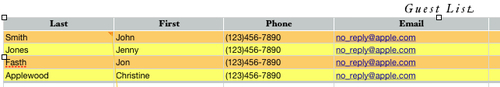
- Go to Table Inspector. Under Cell Background, select Color Fill from the drop-down menu. Check the Alternating Row Color checkbox:
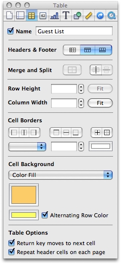
- Click on the large rectangular color well to select the color for the first row in the table grid. When the Colors Viewer opens, click on the Cantaloupe color in the crayons box.
- For the second color, click on the smaller color well that looks like a tab and choose Banana in the crayons box.
Now the table has bright alternating colors.
Next, select the Budget table.
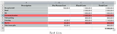
To add a color to one or several rows in the table, follow these steps:
- Click anywhere in the table. This will show reference tabs—numbers for rows and letters for columns.
- Select rows 5 and 8. Click on reference tab 5, press Command, and click on reference tab 8.
- Go to Table Inspector, and under Cell Background | Color Fill, click in the large color well (window).
- When the Colors Viewer opens, click on the pink crayon (Salmon) in the box of crayons. Both row 5 and 8 will turn pink.
Keep the rows colored as a reminder to finish the task—confirm the costs, add a name or address, fill in blank cells, and so on. In this example, organizers may want to check or renegotiate the costs of the highlighted items. Change back to how it was when the task was finished.
Setting cell colors to change on a certain day can help in drawing attention to or quickly identifying areas in our documents that correspond to tasks that need urgent action or special attention. We can use this technique, for example, to remember to send out reminders to clients to pay bills after 30 days or to remind us to pay our own. We can enter a date to submit tax returns, renew a license or passport, take the car for servicing, and so on.
Now, we will use the Task List table from the Event Planner template. In this example, we assume (for demonstration purposes) that today is May 10, 2012. However, you need to use current dates when you follow the steps discussed here, as your spreadsheet is synchronized with your computer's clock.
To set cell colors to change, do this:
- Click on the Task List table. It will show reference tabs.
- Click on reference tab B to select column B.
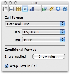
- Go to Cells Inspector, click to open the drop-down menu under Cell Format, and choose Date and Time.
- Click on the Date tab to open the drop-down menu and choose a date display format, for example, 05/08/12 for day, month, and year. For Time, choose None.
- For column B, in rows 2 to 7, type in the following dates:
- B2: March 3, 2012
- B3: June 7, 2012
- B4: May 9, 2012
- B5: April 12, 2012
- B6: March 20, 2012
- B7: February 14, 2012
In the template, this column already has dates. Type anything inside the cell to see the effect of the rule applied to cells with dates.
- In Cells Inspector, click on the Show Rules button to open the Conditional Format control panel:
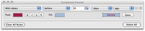
- In the Conditional Format panel, click on the first tab and choose With dates from the drop-down menu to apply the rule to all cells that contain dates.
- Click on the second tab and choose before.
- In the window, type
30. - From the drop-down menu to the right of the window, choose days.
- In the last drop-down menu, choose ago.
- To set a different color for text (dates) in cells with date and time format, click on the Edit button to open text and background options.
- Then, click in the color well (tab) next to Text and choose a shade of red from the color palette. Text will change to this color when 30 days from the date in the cell have expired.
- For the cell background, click in the color well next to Fill and choose a shade of blue. The background color will also change after 30 days.
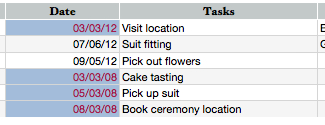
These rules will be applied automatically—cells in the table change as soon as you make your choices. We can see that dates older than 30 days from today's date have changed to red and the cells' background has changed to blue, which reminds us to take appropriate action, such as sending out reminders, paying bills, and so on.
Depending on what you want to do with a table, you can select it without showing reference tabs for rows and columns. Press Shift and then click on a table. This selects the table without showing reference tabs. Small square handles will be shown as they are shown on any selected object in iWork. Drag them to resize the table. If you click on a table without pressing Shift, it will show reference tabs and you can start working with cells, rows, and columns.
To select a row or a column, click on the corresponding reference tab. To select several rows or columns, press Shift when clicking, but this will also select adjacent rows. For example, if you click on row 2, press Shift, and then click on row 5, all rows from 2 to 5 will be selected. To select only rows 2 and 5, press Command when clicking on the rows or columns that you want to select.
The Conditional Format control panel allows several different rules to be applied. Think through your tasks, decide what you want your spreadsheet to do for you, and then decide what rules to set up to help you with this task.