
Chapter 10. Making predictions
In this chapter, we build predictive models. A predictive model makes a prediction for the value of an output attribute using the values associated with other input attributes. Predictive models can be categorized into two types based on whether the predicted attribute is continuous or discrete. When the predicted attribute is discrete, the problem is one of classification, whereas when the attribute is continuous, the problem is one of regression. Some predictive models, as in the case of neural networks, can be built to predict multiple output attributes, while others predict a single attribute.
There are two steps involved with using predictive models: the learning phase and the application phase. In the learning phase, given a dataset of examples where each example has a set of input and output attributes, the learning process tries to build a mathematical model that predicts the output attribute value based on the input values. Once a mathematical model has been built, the second step is to apply the model to make predictions. The application of the mathematical model for predictions is typically fast, and can be used for real-time predictions in an application, while the amount of time taken to build the predictive model is much greater and is typically done asynchronously in the application.
In this chapter, we review some of the key supervised learning algorithms used for both classification and regression. We build on the example from the previous chapter of clustering blog entries. We use a simple example to illustrate the inner workings of the algorithms. We also demonstrate how to build classifiers and predictors by using the WEKA APIs. For this, we apply the APIs to live blog entries retrieved from Technorati. Three commonly used classification algorithms are covered in this chapter: decision trees, Naïve Bayes, and Bayesian networks (also known as belief networks or probabilistic networks). The key regression algorithms covered in this chapter include linear regression, multi-layer perceptron, and radial basis functions. We also briefly review the JDM APIs related to classification and regression. At the end of this chapter, you should have a good understanding of the key classification and regression algorithms, how they can be implemented using the WEKA APIs, and the related key JDM concepts.
10.1. Classification fundamentals
In most applications, content is typically categorized into segments or categories. For example, data mining–related content could be categorized into clustering, classification, regression, attribute importance, and association rules. It’s quite useful, especially for user-generated content, to build a classifier that can classify content into the various categories. For example, you may want to automatically classify blog entries generated by users into one of the appropriate categories for the application.
One common example of a classification problem is email filtering. Here, the classifier predicts whether a given email is spam. The classifier may use a variety of information to make the prediction, such as the name of the sender, the number of individuals the email has been sent to, the content of the email, the prior history of the user interacting with similar emails, the size of the email, and so forth. The process of classifying emails is fairly involved and complex. and there are a number of commercial products that do this task. Therefore, we use a simpler example later in this section to illustrate the classification process.
In this section, we review three of the most commonly used classifiers: decision trees, Naïve Bayes, and belief networks. In Section 10.2, we use WEKA APIs to apply these classifiers to the problem of classifying blog entries.
10.1.1. Learning decision trees by example
Decision trees are one of the simplest and most intuitive classifiers used in the industry. The model generated from a decision tree can be converted to a number of if-then rules, and the relationships between the output attributes and input attributes are explicit. In section 7.1.3, we briefly described a decision tree. In this section, we work through an example to better understand the concepts related to building one.
In our example, we have a number of advertisements that we can potentially show to a user. We want to show the advertisement that the user is most likely to click (and then buy the advertised item). One such advertisement is for an expensive Rolex watch. In our example, we want to build a predictive model that will guide us as to whether we should show this Rolex advertisement to a user. Remember, we want to optimize the likelihood of the user actually buying the item as opposed to simply clicking on the ad to browse the content. In essence, we want to optimize the look-to-book ratio for our product—the proportion of users who’ve looked at an item and who then bought the item.
Based on some past analysis of the kind of people who tend to buy this watch, we’ve identified three attributes—in the real world, you’ll probably have many more:
- Is this a high-net-worth individual?— Our user has provided the ZIP code of his home address during the registration process. We’ve correlated this ZIP code with average home values in that area and have converted this into a Boolean attribute {true, false} indicating whether this individual has a high net worth.
- Is the user interested in watches?— This again is a Boolean attribute. It assumes a value of {true, false}. A user is deemed to be interested in watches if recently (in the current interaction session) the user has either searched for content on the site that has a keyword watch or rolex or has visited content related to these keywords.
- Has the user bought items before?— This again takes a Boolean value {true, false} based on whether the user has transacted before on the site.
Some of the other attributes you can use to build such a predictive model are the user’s gender, the age, the referring page, and so on.
We’ve collected the data of users who clicked on the ad for the watch and whether they actually bought the item. Table 10.1 contains some sample data that we use in our analysis. Note that User 3 and User 4 have the same input attributes but different outcomes. You may want to look at the data to see if you can find any patterns that you can use for predicting whether the user is likely to buy the watch.
Table 10.1. Raw data used in the example
|
High net worth |
Interested in watches |
Has purchased before |
Purchased item |
|
|---|---|---|---|---|
| User 1 | F | T | T | F |
| User 2 | T | F | T | F |
| User 3 | T | T | F | T |
| User 4 | T | T | F | F |
| User 5 | T | T | T | T |
Remember that a decision tree consists of nodes and links. Each node has an associated attribute. The number of links originating from the node equals the number of discrete values that the attribute can take. In our case, all the attributes are binary and take a value of {true, false}. Based on the given data, we need to determine the best attribute that we can use to create the decision tree.
Intuitively, we want to select the attribute that can best predict the output. A commonly used measurement for this is information entropy—this measures the amount of chaos associated with the distribution of values. The lower the entropy, the more uniform the distribution. To see how entropy is calculated, let’s look at the first attribute: high net worth. Splitting the dataset based on the values of this attributes leads to two sets:
- False with output case {F}
- True with output cases {F, T, F, T}
Given a set of p positive cases and n negative cases, we can compute the gain[1] associated with the distribution using the code shown in listing 10.1.
1 Please refer to the references at the end of the chapter for more details on the computation of information entropy and how it came about.
Listing 10.1. Computing the gain associated with a distribution
public double gain(double p, double n) {
   double sum = p+n;
   double gain = p*log2(p/sum)/sum + n*log2(n/sum)/sum;;
   return -gain;
}

private double log2(double x) {
   if (x <= 0.) {
      return 0.;
   }
   return Math.log10(x)/Math.log10(2.);
}
Note that a perfect attribute will be one that splits the cases into either all positives or all negatives—in essence, Gain(1,0) = 0. On the other hand, an attribute that splits the space into two equal segments will have the following information gain: Gain(1,1) = 1.
Let’s calculate the gain associated with the initial set of data, which consist of three negative cases and two positive cases:
| Gain(2, 3) | = (2/5)*log2 (2/5) + (3/5) * log2 (3/5) |
| = 0.97 |
Now, one can compute the entropy associated with splitting on the first attribute, which creates two sets {F} and {F, T, F, T} by the following process:
| Gain(0,1) | = 0 + (1) * log2 (1) |
| = 0 | |
| Gain(2,2) | = (2/4) log2 (2/4) + (2/4) log2(2/4) |
| = 1 |
Both these gains are added in the ratio of the number of samples that appear:
| Net Gain (attribute = high net worth) | = | (1/5) * 0 + (4/5) *1 |
| = | 0.8 |
The overall information gain associated with splitting the data using the first attribute is
| Net Info Gain(attribute = high net worth) | = | Gain(before split) – Gain (after split) |
| = | 0.97 - 0.8 | |
| = | 0.17 |
Similarly, the second attribute, interested in watches, splits the dataset into two sets, which happen to be the same as with the first attribute:
- False with output case {F}
- True with output cases {F, T, F, T}
Therefore, Info Gain(interested in watches) = 0.17
Lastly, the third attribute, has purchased before, splits the dataset into the following two sets:
- False with values {T, F}
- True with values {F, F, T}
| Net Info Gain (attribute = has purchased before} | = | -0.97 – { (2/5) Gain(1,1) + 3/5 Gain(1,2)} |
| = | 0.02 |
Selecting either the first or the second attribute leads to the highest net information gain. We arbitrarily select the first attribute to break this tie. Figure 10.1 shows the first node we’ve created for our decision tree, along with the set of cases that are available for the node.
Figure 10.1. The first node in our decision tree

Next, let’s consider the case when the individual doesn’t have a high net worth. Table 10.2 contains the one case that’s applicable for this node.
Table 10.2. Data available when the user isn’t a high-net-worth individual
|
Interested in watches |
Has purchased items |
Purchased |
|
|---|---|---|---|
| User 1 | T | T | F |
Note that because there’s just one case, all cases have the same predicted value. The information gain even without further splitting is Info Gain(0,1) = 0.
There’s nothing to be gained by further splitting any of the other attributes when the user isn’t a high-net-worth individual. We can safely predict that the user won’t buy the Rolex watch.
Next, let’s consider the case when the user has a high net worth. Table 10.3 shows the data associated with high-net-worth individuals.
Table 10.3. Data available when the user is a high-net-worth individual
|
Interested in watches |
Has purchased items |
Purchased |
|
|---|---|---|---|
| User 2 | F | T | F |
| User 3 | T | F | T |
| User 4 | T | F | F |
| User 5 | T | T | T |
There are two positive cases and two negative cases. The information gain associated with not splitting this node further is Info Gain(2, 2) = 1.
Next, for this dataset, let’s compute the information gain associated with the two remaining attributes: is the user interested in watches, and has the user purchased items before?
Using the attribute interested in watches, we can split the dataset into the following two sets:
- True leads to {True, False, True}
- False leads to {False}
| Net Info Gain | = | 1 – { (3/4) gain(2,1) + (1/4) gain(1,1)} |
| = | 1 – 0.69 | |
| = | 0.31 |
Similarly, splitting the data using the attribute has purchased before, leads to the following two datasets:
- True leads to {False, True}
- False leads to {True, False}
| Net Info Gain | = | 1 – { (1/2) gain(1,1) + (1/2) gain (1,1) } |
| = | 0 |
Note that splitting on interested in watches has the maximum net information gain, and this is greater than zero. Therefore, we split the node using this attribute. Figure 10.2 shows the decision tree and the available data using this attribute for splitting.
Figure 10.2. The second split in our decision tree

Next, let’s consider the case when the user has a high net worth but isn’t interested in watches. Table 10.4 contains the data associated with this case.
Table 10.4. Data when user has high-net-worth individual but is not interested in watches
|
Has purchased items |
Purchased |
|
|---|---|---|
| User 2 | T | F |
Again, there’s only one case, so this falls into the category where all the output cases have the same prediction. Therefore, we can predict that the user won’t buy the Rolex watch for this node.
Next, let’s consider the case that the user has a high net worth and is interested in watches. Table 10.5 shows the set of data available for this node.
Table 10.5. Data when user has high-net-worth individual and is interested in watches
|
Has purchased items |
Purchased |
|
|---|---|---|
| User 3 | F | T |
| User 4 | F | F |
| User 5 | T | T |
First, the information gain by not splitting is Info Gain(2,1) = 0.92.
Splitting on the last attribute, has purchased before, leads to the following two datasets:
- False with cases {True, False}
- True with case {True}
| Net Info Gain(attribute = has purchased items before) | = 0.92 – {(2/3) gain (1,1) + (1/3) gain(1,0)} |
| = 0.59. |
It’s worthwhile to split on this attribute. Remember, we don’t want to over-fit the data. The net information gain associated with splitting on an attribute should be greater than zero.
Figure 10.3 shows the final decision tree. Note that each leaf node can be converted into rules. We can derive the following four rules from the tree by following the paths to the leaf nodes:
- If the user doesn’t have a high net worth then she won’t buy the watch.
- If the user has a high net worth but isn’t interested in watches then she won’t buy the watch.
Figure 10.3. The final decision tree for our example

- If the user has a high net worth and is interested in watches, and has bought items before, then she will buy the watch.
- If the user has a high net worth and is interested in watches, but hasn’t bought items before, then the user might or might not buy the watch, with equal probability.
With these four rules, we can decide whether it’s worthwhile to show the Rolex advertisement for a user who’s visiting our site. Our click-through rates for this ad should be higher than if we decide randomly whether to show the Rolex ad.
The example we’ve just worked through uses attributes with binary values. The same ideas are generalized for attributes with more than two discrete values. CART, ID3, C4.5, and C5.0 are some of the common implementations of decision trees. In section 10.2, we use the WEKA libraries to learn decision trees. Next, we use probability theory to build our next classifier, called Naïve Bayes’ classifier.
10.1.2. Naïve Bayes’ classifier
Before we look at the implementation of the Naïve Bayes’ algorithm, we need to understand a few basic concepts related to probability theory. First, the probability of a certain event happening is a number between zero and one. The higher the number, the greater the chances of that event occurring. One of the easiest ways to compute an event’s probability is to take its frequency count. For example, for the data in table 10.1, in two cases out of five, the individuals bough the watch. Therefore, the probability of a user buying the watch is 2/5 = 0.4.
Next, let’s calculate some probabilities using the data available in table 10.1. We assume that each attribute associated with the user has an underlying probability distribution. By taking the frequency count we have the probabilities shown in table 10.6.
Table 10.6. Computing the probabilities
|
Value=True |
Value=False |
|
|---|---|---|
| High net worth | 4/5 = 0.8 | 1/5 =0.2 |
| Interested in watches | 4/5 = 0.8 | 1/5 = 0.2 |
| Has purchased before | 3/5 = 0.6 | 2/5 = 0.4 |
Now, let’s find the probability that a user is both a high-net-worth individual and is interested in watches. The last three rows in table 10.1 are of interest to us. Hence, this probability is 3/5 = 0.6.
What if we wanted to find out the probability that a user is either a high-net-worth individual or is interested in watches (or both)? Again, looking at the data in table 10.1, we’re interested in all the rows that have True in either the first or second column. In this case, all five rows are of interest to us, and the associated probability is 5/5 = 1.0.
But we could have computed the same information by adding the probability of a user being a high-net-worth individual (0.8) and the probability of the user being interested in watches (0.8) and subtracting the probability of both these attributes being present together (0.6):
= 0.8 + 0.8 – 0.6 = 1.0
More formally, the probability associated with either of the two variables occurring is the sum of their individual probabilities, subtracting the probability of both variables occurring:
Pr{A or B } = Pr{A} + Pr{B} – Pr{A and B}
Next, let’s say that we want to compute the probability of A and B occurring. This can happen in one of two ways:
- Variable A occurs and then variable B occurs.
- Variable B occurs and then variable A occurs.
We use the notation Pr{B | A} to refer to the probability of B occurring, given that A has already occurred. Thus, the probability of A and B occurring can be computed as
| Pr{A and B} | = Pr{A}Pr{B|A} |
| = Pr{B} Pr{A|B} |
This formula is also known as Bayes’ Rule and is widely used in probability-based algorithms. Again, it’s helpful to work through some concrete numbers to better understand the formulas.
Following this formula:
| Pr{high net worth and interested in watches} | |
| = Pr{high net worth} Pr{interested in watches | high net worth} | |
| = Pr{interested in watches} Pr {high net worth | interested in watches} | |
To compute the conditional probability Pr {interested in watches | high net worth}, we need to look at the bottom four rows that have True in the first column. When the individual has high net worth, in three cases out of four, the user is interested in watches. Hence, the conditional probability is 3/4 = 0.75. Similarly, the conditional probability of the user having a high net worth given that the user is interested in watches is three out of four: 3/4 = 0.75.
Substituting the values, we get
| Pr{high net worth and interested in watches} | |
| = 0.8 * 0.75 | |
| = 0.8 * 0.75 | |
| = 0.6 | |
With this basic overview of probability theory, we’re now ready to apply it to the problem of classification. Our aim is to calculate the probability of a user buying a watch, given the values for the other three attributes. We need to shorten the description for the attributes. For the sake of brevity, let’s call the three attributes A, B, and C, and the predicted attribute P, as shown in table 10.7.
Table 10.7. Shortening the attribute descriptions
|
Description |
|
|---|---|
| A | Is the user a high-net-worth individual? |
| B | Is the user interested in watches? |
| C | Has the user bought items before? |
| P | Will the user buy the watch? |
Let’s assume that a user who has a high net worth, is interested in watches, and has purchased items before is visiting the site. We want to predict the probability that the user will buy the item:
Pr {P=T | A=T,B=T,C=T} = Pr {A=T,B=T, C= T | P = T} Pr{T}/ Pr {A=T,B=T, C= T }
Pr {P=F | A=T,B=T,C=T} = Pr {A=T,B=T, C= T | P = F} Pr{F}/ Pr {A=T,B=T, C= T }
Computing Pr {A=T,B=T, C= T | P = T} is typically not that easy, especially with a large number of attributes and when the learning data is sparse.[2] To simplify matters, we assume that all three attributes are conditionally independent of each other, given the output attribute. Therefore, to compute Pr {A=T,B=T, C= T | P = T}, let’s first split the examples into two sets based on the value of the output variable, as shown in figure 10.4.
2 For example, note that there is no data in our dataset to compute Pr {A=F,B=T, C= T | P = T}.
Figure 10.4. Splitting the dataset based on the value of the output attributes to compute the conditional probabilities

Using the cases where the output attribute is True, we can calculate the following conditional probabilities:
- Pr {A = T | P = T} = 1
- Pr {B = T | P = T} = 1
- Pr {C = T | P = T} = 1/2
- Pr {A = F | P = T} = 0
- Pr {B = F | P = T} = 0
- Pr {C = F | P = T} = 1/2
Similarly, using the cases where the output attribute if False, we can calculate the following conditional probabilities:
- Pr {A = T | P = F} = 2/3
- Pr {B = T | P = F} = 2/3
- Pr {C = T | P = F} = 2/3
- Pr {A = F | P = F} = 1/3
- Pr {B = F | P = F} = 1/3
- Pr {C = F | P = F} = 1/3
Also, the prior probabilities are as follows:
Pr {P = T} = 0.4 and Pr {P = F} = 0.6
Hence, we can calculate Pr {A=T, B=T, C= T | P = T}:
| Pr {A=T,B | =T, C= T | P = T} = Pr {A=T | P = T} Pr {B=T | P = T} Pr {C=T | P = T} |
| = 1 * 1 * (1/2) = (1/2) |
Here, we’ve simply expanded the formula and substituted the known values. Similarly:
| Pr {A=T,B | =T, C= T | P = F} = Pr {A=T | P = F} Pr {B=T | P=F} Pr{C=T | P=F} |
| = (2/3) * (2/3) * (2/3) = 8/27 |
The likelihood of a user buying the watch can be computed as follows:
| Pr {P=T | A | =T,B=T,C=T}/ Pr {P=F | A=T,B=T,C=T} |
| = Pr {A=T,B=T, C= T | P = T} Pr{T}/ Pr {A=T,B=T, C= T | P = F} Pr{F} | |
| =(1/2)*(2/5)/ {(8/27)* (3/5)) | |
| = 27/24 | |
| = 9/8 |
This implies that the user is more likely to buy the watch when all three conditions are met. This prediction is the same as one of the nodes that was derived by the decision tree.
When the conditional independence assumption is used, the algorithm is known as Naïve Bayes.
The probability-based approach can handle missing variables. For example, let’s say that we don’t know whether the individual has a high net worth. In this case, we can calculate the likelihood of the user buying the watch as
| Pr {P=T | B | =T,C=T}/ Pr {P=F | B=T,C=T} |
| = Pr {B=T, C= T | P = T} Pr{T}/ Pr { B=T, C= T | P = F} Pr{F} | |
| = (1/2)*(2/5)/ {(1/3)*(3/5)} | |
| = 0.5 |
In this case, a user is more likely to not buy the watch—a value of 1 would imply an equal chance between buying and not buying. Given that we only have three binary inputs and there are only (23 = 8) cases, we can summarize the probabilities and make a prediction for each case. This is shown in table 10.8.
Table 10.8. The prediction table for our example
|
High net worth |
Interested in watches |
Has purchased |
Will buy = True |
Will buy = False |
Prediction |
|---|---|---|---|---|---|
| T | T | T | 1/5 | 8/45 | Buy |
| T | T | F | 1/5 | 4/45 | Buy |
| T | F | T | 0 | 4/45 | Not Buy |
| T | F | F | 0 | 2/45 | Not Buy |
| F | T | F | 0 | 4/45 | Not Buy |
| F | T | F | 0 | 2/45 | Not Buy |
| F | F | T | 0 | 2/45 | Not Buy |
| F | F | F | 0 | 1/45 | Not Buy |
Note that the sum of the probabilities for predicted value being true is = (1/5 + 1/5) = 0.4, and the probability for the predicted value being false is 27/45 = 0.6, which is equal to the a priori probability—the probability of the two events occurring in the absence of any evidence. Also, in the second row in table 10.8—when the user has a high net worth and is interested in watches but hasn’t bought items before (A = T & B = T & C = F)—the Naïve Bayes’ analysis predicts that the user is more likely to buy the watch, with a likelihood of 9/4. You may recall that in the previous section, using the decision tree, the prediction had an equal likelihood of the user buying the watch.
Even though the Naïve Bayes’ process is simple, it’s known to give results as good as, if not better than, some of the other, more complicated classifiers. The probability-based approach can be generalized and represented using a graph. The resulting network is commonly known as a Bayesian belief network, also called probabilistic reasoning, which we look at next.
10.1.3. Belief networks
Belief networks are a graphical representation for the Naïve Bayes’ analysis that we did in the previous section. More formally, a belief network is a directed acyclic graph (DAG) where nodes represent random variables, and links between the nodes correspond to conditional dependence between child and parent nodes. Each variable may be discrete, in which case it assumes an arbitrary number of mutually exclusive and collectively exhaustive values, or it may be continuous. The absence of an arrow between two nodes represents conditional independence between the variables. The network is directed—there’s a direction associated with the nodes—and acyclic—there are no cycles between the connections. Each node has a conditional probability table that quantifies the effects that the parents have on the node. The parents of a node are all those nodes that have arrows pointing to them. For our example, belief networks are best illustrated using a graphical representation.
Figure 10.5 shows the belief network for our example. Note the following:
Figure 10.5. Belief network representation for our example

- The arrow from P, the predicted attribute, to the three children nodes A, B, and C implies that when P occurs, it has an effect on each of its children. There’s a causal or cause-effect relationship between the parent and the child node.
- Associated with each variable is a conditional probability table. The node P has no parents and the associated probabilities with the node are known as a priori probabilities.
- Given the parent, P, the three children nodes A, B, and C are assumed to be conditionally independent of each other.
In the absence of any additional information about the values for A, B, and C, the network predicts the probability of Pr {P = T} = 0.4. Let’s say that we know that the person has a high net worth: A = T. With this new evidence, what’s the new probability associated with P? Figure 10.6 shows the belief network associated with this case. There are just two nodes in the network.
Figure 10.6. The simplified belief network when only A is known

From this, we can compute the following:
| Pr {P | = | T | A = T} = Pr {A = T| P = T} Pr {P = T}/Pr {A = T} |
| = | 1 * (0.4) / 1. = 0.4 |
This is the same as when we didn’t know whether A was True. However, if we knew that A = False, we can compute the following:
| Pr {P | = | T | A = F} = Pr {A = F| P = T} Pr {P = T}/Pr {A = F} |
| = | 0 * (0.4) / 1. = 0 |
Doing the inference in the network to take into account new evidence amounts to applying the Bayes’ Rule, and there are well-known algorithms for doing this computation. Belief networks can be singly or multiply connected. An acyclic graph is singly connected if there’s at most one chain (or undirected path) between a pair of variables. Networks with undirected cycles are multiply connected.
There are a number of inference algorithms for a simply-connected network. There are three basic algorithms for evaluating multiply connected networks: clustering methods, conditioning methods, and stochastic simulation. There are also well-known algorithms for constructing belief networks using test data. Expert-developed belief networks have been used extensively in building knowledge-based systems.
At this point, it’s helpful to review the Bayesian interpretation of probability. One prevalent notion of probability is that it’s a measure of the frequency with which an event occurs. A different notion of probability is the degree of belief held by a person that the event will occur. This interpretation of probability is called subjective or Bayesian interpretation.
We’re done with our Rolex advertisement example. In the next section, we use a new example, classifying blog entries, to illustrate the use of WEKA APIs for classification.
10.2. Classifying blog entries using WEKA APIs
In this section, we build on our example of clustering blog entries from the previous chapter. We demonstrate the process of classification by retrieving blog entries from Technorati on a variety of topics. We categorize the blog entries into two sets—one of interest to us and the other not of interest to us. In this section, we apply a variety of classifiers, using the WEKA APIs to classify the items into the two categories. Later in the chapter, when we deal with regression, we use the same example to build predictors, after converting the attributes into continuous attributes. At the end of this section, you should be familiar with the classification process and the use of WEKA APIs to apply one of many classification algorithms.
Figure 10.7 outlines the four classes that we use in this chapter. You may recall that BlogDataSetCreatorImpl, which we developed in section 9.1.2, is used to retrieve blog entries from Technorati. WEKAPredictiveBlogDataSetCreatorImpl extends this class and creates the dataset that’s used for classification and regression. WEKABlogClassifier is a wrapper class to WEKA, which invokes the WEKA APIs to classify blog entries using the dataset created by WEKAPredictiveBlogDataSetCreatorImpl. In section 10.5,
Figure 10.7. The classes that we develop in this chapter

we extend WEKABlogClassifier to create WEKABlogPredictor, which is used for invoking WEKA regression APIs.
Next, let’s look at the implementation for the first of our classes, WEKAPredictiveBlogDataSetCreatorImpl.
10.2.1. Building the dataset for classifying blog entries
Classification algorithms typically deal with nominal or discrete attributes, while regression algorithms normally deal with continuous attributes. We build predictive models to predict whether a blog entry is of interest. To create the dataset for learning, we do the following:
- Retrieve blog entries from Technorati for a set of tags. Blog entries associated with each tag are marked to be either an item of interest or an item in which we aren’t interested.
- Similar to our approach in chapter 9, we parse through the retrieved blog entry to create a term vector representation for each of the blog entries. Each term vector is associated with the predicted value of whether this entry is of interest.
- Each term vector gets converted into the WEKA Instance object. A collection of these Instance objects forms the dataset and is represented by the Instances object.
- For nominal attributes, we convert each of the tags into a Boolean attribute, which takes a value of true if the tag appears in the blog entry and a value of false if it’s absent. Of course, you can use more sophisticated techniques to discretize the term vector into categorical attributes.
Listing 10.2 shows the first part of the code for WEKAPredictiveBlogDataSetCreatorImpl, which deals with creating the dataset with positive and negative test cases.
Listing 10.2. Retrieving blogs

To create the dataset, we specify a set of positive and negative test cases. For example, in the code
String [] positiveTags = { "collective intelligence",
  "data mining", "web 2.0"};
String [] negativeTags = { "child intelligence", "AJAX"};
we retrieve blog entries from Technorati using the following tags for the positive cases—collective intelligence, data mining, and web 2.0—and the following tags for the negative cases—child intelligence and AJAX.
The method getBlogData() uses the specified tag to retrieve relevant blog entries from Technorati, and predicts whether they’ll be relevant. Of course, we’re really interested in getting a WEKA dataset representation—an instance of Instances using the retrieved blog entries. For this, we need to look at listing 10.3.
Listing 10.3. Creating the dataset
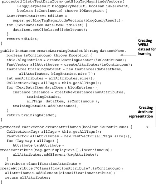
There’s only one public method in the class WEKAPredictiveBlogDataSetCreatorImpl: createLearningDataSet(). This method takes in a name for the dataset and whether we want continuous or discrete attributes. It first retrieves all the blog entries from Technorati, creates an attribute representation, and creates the dataset by converting each blog entry into an Instance object.
The method createAttributes() creates an Attribute representation for each tag by invoking the similarly named createAttribute() method. Details of create-Attribute() are shown in listing 10.4.
Listing 10.4. Creating Instance in WEKAPredictiveBlogDataSetCreatorImpl

The method createAttribute() creates either discrete or continuous attributes based on the isContinuous flag. The method createNewInstance() creates a new instance for each blog entry. It iterates over all the tags and sets the instance value through the method setInstanceValue(). The value associated with an attribute in an instance is either true or false for discrete attributes, or the magnitude of the term in the term vector for continuous attributes.
Now that we have a dataset that can be used for learning, let’s look at how we can leverage the WEKA APIs to apply various classification algorithms on this dataset.
10.2.2. Building the classifier class
In this section, we build a wrapper class for calling the WEKA APIs. WEKABlogClassifier is a generic class that, given an Algorithm, creates the dataset for learning, creates an instance of the classifier, builds the classifier using the available data, and then evaluates it. Listing 10.5 shows the implementation for the WEKABlogClassifier class.
Listing 10.5. The implementation of the WEKABlogClassifier class

We first define an enumeration, Algorithm, that contains some of the classifier and regression algorithms supported by WEKA. Note that WEKA supports many more algorithms—more than 50. The method to classify blog entries is fairly straightforward:
public void classify(Algorithm algorithm) throws Exception
It consists of three steps:
1. Creating the dataset to be used for learning
2. Getting the classifier instance based on the specified algorithm and building the model
3. Evaluating the model that’s created
Note that for classification and regression algorithms, you need to specify the predicted output attribute. We do this in the method getClassifier:
instances.setClassIndex(instances.numAttributes() - 1);
It’s helpful to look at the output from our classification process. Listing 10.6 shows the output from one of the runs. It shows a decision tree that correctly classified 55 of the 60 blog entries presented to it. The details of the decision tree are also shown (using System.out.println(((J48)classifier).graph());).
Listing 10.6. Sample output from a decision tree
Results
=======

Correctly Classified Instances        55           91.6667 %
Incorrectly Classified Instances       5            8.3333 %
Kappa statistic                        0.8052
Mean absolute error                    0.1425
Root mean squared error                0.267
Relative absolute error               31.9444 %
Root relative squared error           56.6295 %
Total Number of Instances             60

digraph J48Tree {
N0 [label="ci" ]
N0->N1 [label="= true"]
N1 [label="true (6.0)" shape=box style=filled ]
N0->N2 [label="= false"]
N2 [label="review" ]
N2->N3 [label="= true"]
N3 [label="true (3.0)" shape=box style=filled ]
N2->N4 [label="= false"]
N4 [label="machine" ]
N4->N5 [label="= true"]
N5 [label="true (3.0)" shape=box style=filled ]
N4->N6 [label="= false"]
N6 [label="technology" ]
N6->N7 [label="= true"]
N7 [label="true (3.0/1.0)" shape=box style=filled ]
N6->N8 [label="= false"]
N8 [label="web" ]
N8->N9 [label="= true"]
N9 [label="online" ]
N9->N10 [label="= true"]
N10 [label="false (2.0)" shape=box style=filled ]
N9->N11 [label="= false"]
N11 [label="true (2.0)" shape=box style=filled ]
N8->N12 [label="= false"]
N12 [label="false (41.0/4.0)" shape=box style=filled ]
}
In this specific example, the root node, N0, is with the term "ci". When the blog contains the term "ci", it gets classified into the node N1, which has a "true" prediction; if the blog doesn’t have the term, it leads to node N2. The node N2 has two children nodes, N3 and N4. One can follow down the node hierarchy to visualize the generated decision tree.
Later in section 10.5, we discuss JDM APIs related to the classification process. So far, we’ve looked at building predictive models for discrete attributes. Next, let’s briefly look at building predictive models for continuous attributes.
10.3. Regression fundamentals
Perhaps the simplest form of predictive model is to use standard statistical techniques, such as linear or quadratic regression. Unfortunately, not all real-world problems can be modeled as successfully as linear regression; therefore more complicated techniques such as neural networks and support vector machine (SVM) can be used. The process of building regression models is similar to classification algorithms, the one difference being the format of the dataset—for regression, typically all the attributes are continuous. Note that regression algorithms can also be used for classification, where the predicted numeric value is mapped to an appropriate categorical value.
In this section, we briefly review linear regression, and follow with an overview of two commonly used neural networks—the multi-layer perceptron and the radial basis function. In the next section, we use the WEKA APIs for regression.
10.3.1. Linear regression
In linear regression, the output value is predicted by summing all values of the input attributes multiplied by a constant. For example, consider a two-dimensional space with x and y axes. We want to build a linear model to predict the y value using x values. This in essence is the representation of a line. Therefore
y = a x + b
= [x 1] [a b]T
where a and b are constants that need to be determined.
We can generalize this equation into a higher dimension using a matrix representation. Let Y, A, and X be matrices such that
Y = A X
Note that ATA is a square matrix. The constant X can be found
X = (ATA)-1 (ATY)
A concrete example helps to visualize and understand the process of linear regression. To illustrate this process, we use the same example of a Rolex ad that we used earlier in the chapter. Table 10.9 shows the data that we use for our example. This is the same as table 10.1, except that we’ve converted the True values into 1.0 and False values into 0. Note the data for rows corresponding to User 3 and User 4—the input attribute values for both cases are the same but the output is different.
Table 10.9. The data used for regression
|
High net worth |
Interested in watches |
Has purchased items |
Bought the item |
|
|---|---|---|---|---|
| User 1 | 0 | 1 | 1 | 0 |
| User 2 | 1 | 0 | 1 | 0 |
| User 3 | 1 | 1 | 0 | 1 |
| User 4 | 1 | 1 | 0 | 0 |
| User 5 | 1 | 1 | 1 | 1 |
Let, Y be the predicted value, which in our case is whether the user will buy the item or not, and let x0, x1, x2, and x3 correspond to the constants that we need to find. Based on the data in table 10.9, we have

Note that the matrix ATA is a square matrix with a number of rows and columns equal to the number of parameters being estimated, which in this case is four.
Now, we need to compute the inverse of the matrix. The inverse of a matrix is such that multiplying the matrix and its inverse gives the identity matrix. Refer to any book on linear algebra on how to compute the inverse of a matrix.[3]
3 Or use an online matrix inverter such as http://www.bluebit.gr/matrix-calculator/ and http://www.unibonn.de/~manfear/matrixcalc.php for matrix multiplication. The weka.core.matrix.Matrix class in WEKA provides a method to compute the inverse of a matrix.
And its inverse is

Also, ATy = [ 2 2 2 1]
Solving for the four constants, we come to the following predictor model:
P = -1.5 + 1*A + 1*B + 0.5*C
The predicted values for the five cases are shown in table 10.10. Our linear regression–based predictive model does pretty well in predicting whether the user will purchase the item. Note that the predictions for User 3 and User 4 are the average of the two cases in the dataset.
Table 10.10. The raw and the predicted values using linear regression
|
Purchased the item |
Prediction |
|
|---|---|---|
| User 1 | 0 | 0 |
| User 2 | 0 | 0 |
| User 3 | 1 | 0.5 |
| User 4 | 0 | 0.5 |
| User 5 | 1 | 1 |
Building a predictive model using linear regression is simple, and, based on the data, may provide good results. However, for complex nonlinear problems, linear-regression-based predictive models may have problems generalizing. This is where neural networks come in: They’re particularly useful in learning complex functions. Multi-layer perceptron (MLP) and radial basis function (RBF) are the two main types of neural networks, which we look at next.
10.3.2. Multi-layer perceptron (MLP)
A multi-layer perceptron has been used extensively for building predictive models. As shown in figure 10.8, an MLP is a fully-connected network in which each node is connected to all the nodes in the next layer. The first layer is known as an input layer and the number of nodes in this layer is equal to the number of input attributes. The second layer is known as a hidden layer and all nodes from the input layer connect to the hidden layer. In figure 10.8 there are three nodes in the hidden layer.
Figure 10.8. A multi-layer perceptron with one hidden layer. The weight Wxy is the weight from node x to node y. For example, W25 is the weight from node 2 to node 5.

The input feeds into each of the first-layer nodes. The output from a node is split into two computations. First, the weighted sum of the input values of a node is calculated. Next, this value is transformed into the output value of the nodes using a nonlinear activation function. Common activation functions are the sigmoid and the tan hyperbolic functions. The advantage of using these activation functions is that their derivatives can be expressed as a function of the output. Also associated with each node is a threshold that corresponds to the minimum total weighted input required for that node to fire an output. It’s more convenient to replace the threshold with an extra input weight. An extra input whose activation is kept fixed at -1 is connected to each node. Linear outputs are typically used for the output layer.
For example, the output from node 3 is computed as
Activation function (W13 * value of node 1 + W23 * value of node 2 – W03)
The back-propagation algorithm is typically used for training the neural network. The algorithm uses a gradient search technique to find the network weight that minimizes the sum-of-square error between the training set and the predicted values. During the training process, the network is initialized with random weights. Example inputs are given to the network; if the network computes an output vector that matches the target, nothing is done. If there’s a difference between the output and the target vector, the weights are changed in a way that reduces the error. The method tries to assess blame for the error and distributes the error among contributing weights. The algorithm uses a batch mode, where all examples are shown to the network. The corresponding error is calculated and propagated through the network. A net gradient direction is then defined that equals the sum of the gradients for each example. A step is then taken in the direction opposite to this gradient vector. The step size is chosen such that the error decreases with each step. The back-propagation algorithm normally converges to a local optimal solution; there’s no guarantee of a global solution.
A neural network with a large number of hidden nodes is in danger of overfitting the data. Therefore, the process of cross-validation with a test dataset is used to avoid over-learning. Unlike linear regression, an MLP is a “black box” where it’s difficult to interpret the parameters of the network, and consequently it’s difficult to understand the rationale of a prediction made by a neural network. An MLP network requires a large amount of time to train the parameters associated with the network, but once the network has been trained, the computation of the output from the network is fast. An MLP works well when the problem space is large and noisy.
Next, let’s look at another type of commonly used neural network: radial basis functions.
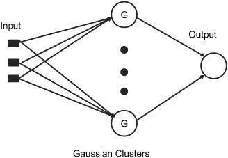
10.3.3. Radial basis functions (RBF)
An RBF, as shown in figure 10.9, consists of two different layers. The inputs feed into a hidden layer. The hidden layer produces a significant nonzero response only when the input vector falls within a small localized region of the input space. The output layer supplies the network’s response to the activation patterns applied to the input layer. The transformation from the input space to the hidden unit space is nonlinear, whereas the transformation from the hidden unit space to the output space is linear. The most common basis for the hidden nodes is the Gaussian kernel function. The node outputs are in the range of zero to one, so that the closer the input is to the center of the Gaussian cluster, the larger the response of the node. Each node produces an identical output that lies a fixed radial distance from the center of the kernel. The output layer nodes form a weighted linear combination of the outputs from the Gaussian clusters.
Figure 10.9. A typical radial basis function
Learning in the RBF network is accomplished by breaking the problem into two steps:
1. Unsupervised learning in the hidden layer
2. Supervised learning in the output layer
The k-means algorithm (see section 9.1.3) is typically used for learning the Gaussian clusters. K-means is a greedy algorithm for finding a locally optimal solution, but it generally produces good results and is efficient and simple to implement. Once learning in the hidden layer is completed, learning in the output layer is done using either the back-propagation algorithm or the matrix inversion process we identified in section 10.3.1. The output from the output node is linear. The connection weights to the output node from the Gaussian clusters can be learned using linear regression. One advantage of RBF over MLP is that learning tends to be much faster.
In theory, the RBF network, like the MLP, is capable of forming an arbitrary close approximation to any continuous nonlinear mapping. The primary difference between the two is the nature of their basis functions. The hidden layer in an MLP forms sigmoidal basis functions that are nonzero over an infinitely large region of the input space; the basis functions in the RBF network cover only small localized regions.
With this overview of some of the key regression algorithms, let’s look at how to apply regression using the WEKA APIs.
10.4. Regression using WEKA
In this section, we use the WEKA APIs to build predictive models using regression. The section is similar to section 10.2; in fact most of the heavy lifting has already been done. As discussed in section 10.2 and in figure 10.7, we simply need to implement WEKABlogPredictor, which is shown in listing 10.7.
Listing 10.7. Implementing regression using the WEKA APIs
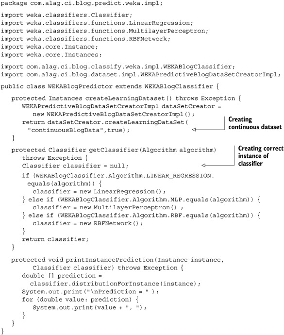
We simply need to overwrite two methods from the parent WEKABlogClassifier class. First, in the method createLearningDataset(), we pass in parameters indicating that we want to create continuous attributes. Second, we need to overwrite the getClassifier() method to get the appropriate classifier based on the specified algorithm. The listing shows the code for creating instances for three of the algorithms covered in this chapter: linear regression, MLP, and RBF.
So far we’ve looked at how we can build predictive models for both the discrete and continuous attributes. Next, let’s briefly look at how the standard JDM APIs deal with classification and regression.
10.5. Classification and regression using JDM
In this section, we briefly review the key JDM interfaces related to classification and regression algorithms. The javax.datamining.supervised package contains the interfaces for representing the supervised learning model. It also contains subpack-ages for classification and regression.
This section is analogous to section 9.3, where we covered JDM-related APIs for clustering. This section covers JDM-related APIs for supervised learning—both classification and regression. We begin by looking at the key JDM supervised learning interfaces. This is followed by developing code to build and evaluate predictive models.
10.5.1. Key JDM supervised learning–related classes
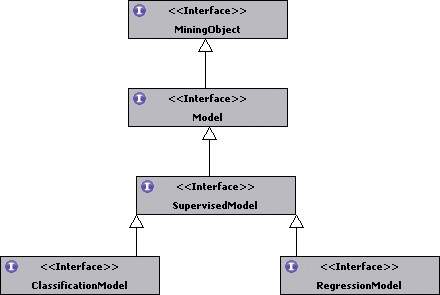
As shown in figure 10.10, the results from supervised learning create either a ClassificationModel or a RegressionModel. Both models have a common parent, Super-visedModel, which extends Model and is a MiningObject.
Figure 10.10. The model interfaces corresponding to supervised learning
For building a supervised learning model, there are two types of settings: SupervisedSettings and SupervisedAlgorithmSettings.
SupervisedSettings, as shown in figure 10.11, are generic settings associated with the supervised learning process. ClassificationSettings extends this interface to contain generic classification-related settings. It supports methods for setting the cost matrix and prior probabilities that may be used by the classifier. RegressionSettings also extends SupervisedSettings and contains generic regression-related settings.
Figure 10.11. Setting interfaces related to supervised learning

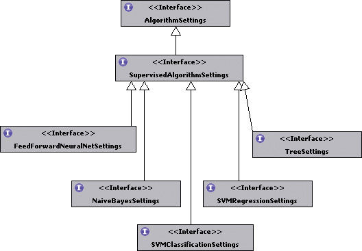
Settings that are specific to a particular algorithm extend the AlgorithmSettings interface. SupervisedAlgorithmSettings, which extends AlgorithmSettings as shown in figure 10.12, is a common interface for all algorithm-related settings. Feed-ForwardNeuralNetSettings, NaiveBayesSettings, SVMClassificationSettings, SVMRegressionSettings, and TreeSettings are five specific algorithm settings.
Figure 10.12. Algorithm-specific settings related to supervised learning algorithms
Next, let’s walk through some sample code that will illustrate the process of creating predictive models using the JDM APIs.
10.5.2. Supervised learning settings using the JDM APIs
In this section, we follow an approach similar to section 9.3.2, which illustrated the use of JDM APIs for clustering. The process for regression and classification is similar; we illustrate the process for classification.
We work through an example that has the following five steps:
1. Create the classification settings object.
2. Create the classification task.
3. Execute the classification task.
4. Retrieve the classification model.
5. Test the classification model.
Listing 10.8 shows the code associated with the example and the settings process.
Listing 10.8. Settings-related code for the classification process
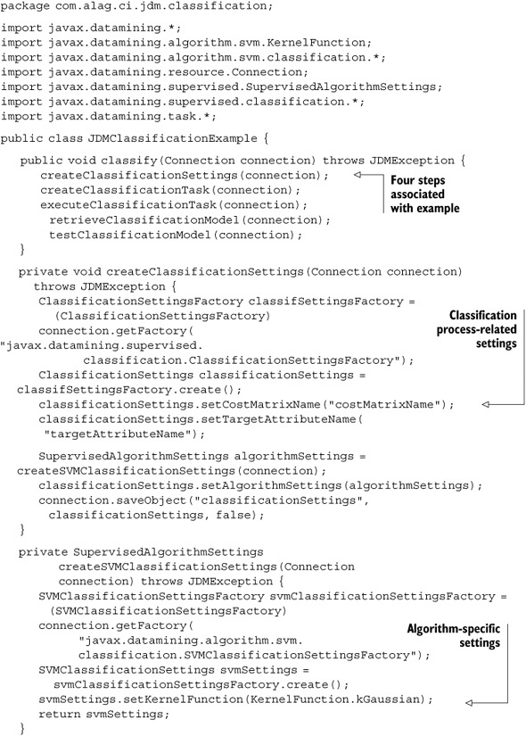
The example first creates an instance of ClassificationSettings and sets attributes associated with the classification process. For this, it sets the cost matrix and the name of the target attribute:
classificationSettings.setCostMatrixName("costMatrixName");
classificationSettings.setTargetAttributeName("targetAttributeName");
Next, an instance of SVMClassificationSettings is created to specify settings specific to the SVM classification algorithm. Here, the kernel function is specified to be Gaussian:
svmSettings.setKernelFunction(KernelFunction.kGaussian);
The algorithm settings are set in the ClusteringSettings instance:
classificationSettings.setAlgorithmSettings(algorithmSettings);
Next, let’s look at creating the classification task.
10.5.3. Creating the classification task using the JDM APIs
To create an instance of BuildTask for clustering, we use the BuildTaskFactory as shown in listing 10.9.
Listing 10.9. Create the classification task
private void createClassificationTask(Connection connection)
  throws JDMException {
   BuildTaskFactory buildTaskFactory = (BuildTaskFactory)
      connection.getFactory(
     "javax.datamining.task.BuildTaskFactory");
   BuildTask buildTask = buildTaskFactory.create(
    "buildDataPhysicalDataSet",
         "classificationSettings", "classificationModel");
   connection.saveObject("classificationBuildTask", buildTask, false);
}
The BuildTaskFactory creates an instance of the BuildTask. The create() method to create a BuildTask needs the name of the dataset to be used, the name of the settings object, and the name of the model to be created. In our example, we use the dataset buildDataPhysicalDataSet, the setting specified in the object classificationSettings, and the model name classificationModel.
10.5.4. Executing the classification task using the JDM APIs
To execute a build task, we use the execute method on the Connection object, as shown in listing 10.10.
Listing 10.10. Execute the classification task
private void executeClassificationTask(Connection connection)
     throws JDMException {
   ExecutionHandle executionHandle =
   connection.execute("classificationBuildTask");
   int timeoutInSeconds = 100;
   ExecutionStatus executionStatus = executionHandle.
    waitForCompletion(timeoutInSeconds);
   executionStatus = executionHandle.getLatestStatus();
   if (ExecutionState.success.equals(executionStatus.getState())) {
      //successful state
   }
}
The code
   ExecutionStatus executionStatus =
executionHandle.waitForCompletion(timeoutInSeconds);
waits for the completion of the classification task and specifies a timeout of 100 seconds. Once the task completes, it looks at execution status to see if the task was successful.
Next, let’s look at how we can retrieve the classification model that has been created.
10.5.5. Retrieving the classification model using the JDM APIs
Listing 10.11 shows the code associated with retrieving a ClassificationModel using the name of the model and a Connection instance.
Listing 10.11. Retrieving the classification model
  private void retrieveClassificationModel(Connection connection)
      throws JDMException {
     ClassificationModel classificationModel = (ClassificationModel)
        connection.retrieveObject("classificationModel",
        NamedObject.model);
     double classificationError = classificationModel.
       getClassificationError();
  }
}
Once a ClassificationModel is retrieved, we can evaluate the quality of the solution using the getClassificationError() method, which returns the percentage of incorrect predictions by the model.
10.5.6. Retrieving the classification model using the JDM APIs
Listing 10.12 shows the code to compute the test metrics associated with the classification model.
Listing 10.12. Testing the classification model
private void testClassificationModel(Connection connection)
   throws JDMException {
  ClassificationTestTaskFactory testTaskFactory =
   (ClassificationTestTaskFactory)connection.getFactory(
   "javax.datamining.supervised.classification.ClassificationTestTask");

  ClassificationTestTask classificationTestTask =
   testTaskFactory.create("testDataName", "classificationModel",
   "testResultName");
  classificationTestTask.computeMetric(
   ClassificationTestMetricOption.confusionMatrix);
  }
The ClassificationTestTask is used to test a classification model to measure its quality. In this example, we’re testing the confusion matrix—a two-dimensional matrix that indicates the number of correct and incorrect predications a classification algorithm has made.
The JDM specification contains additional details on applying the model; for more details on this, please refer to the JDM specification.
In this section, we’ve looked at the key interfaces associated with supervised learning and the JDM APIs. We’ve looked at some sample code associated with creating classification settings, creating and executing a classification task, retrieving the classification model, and testing the classification model.
10.6. Summary
In your application, you’ll come across a number of cases where you want to build a predictive model. The prediction may be in the form of automatically segmenting content or users, or predicting unknown attributes of a user or content.
Predictive modeling consists of creating a mathematical model to predict an output attribute using other input attributes. Predictive modeling is a kind of supervised learning where the algorithm uses training examples to build the model. There are two kinds of predictive models based on whether the output attribute is discrete or continuous. Classification models predict discrete attributes, while regression models predict continuous attributes.
A decision tree is perhaps one of the simplest and most commonly used predictive models. Decision tree learning algorithms use the concept of information gain to identify the next attribute to be used for splitting on a node. Decision trees can be easily converted into if-then rules. The Naïve Bayes’ classifier uses concepts from probability theory to build a predictive model. To simplify matters, it assumes that given the output, each of the input attributes are conditionally independent of the others. Although this assumption may not be true, in practice it often produces good results. Bayes’ networks or probabilistic reasoning provide a graphical representation for probability-based inference. Bayes’ networks deal well with missing data.
In linear regression, the output attribute is assumed to be a linear combination of the input attributes. Typically, the process of learning the model constants involves matrix manipulation and inversion. MLP and RBF are two types of neural networks that provide good predictive capabilities in nonlinear space.
The WEKA package has a number of supervised learning algorithms, both for classification and regression. The process of classification consists of first creating an instance of Instances to represent the dataset, followed by creating an instance of a Classifier and using an Evaluation to evaluate the classification results.
The process of classification and regression using the JDM APIs is similar. Classification with the JDM APIs involves creating a ClassificationSettings instance, creating and executing a ClassificationTask, and retrieving the ClassificationModel that’s created.
Now that we have a good understanding of classification and regression, in the next chapter we look at intelligent search.
10.7. Resources
Alag, Satnam. A Bayesian Decision-Theoretic Framework for Real-Time Monitoring and Diagnosis. 1996. Ph.D dissertation. University of California, Berkeley.
Jensen, Finn. An Introduction to Bayesian Networks. 1996. Springer-Verlag.
Quinlan, J. Ross. C4.5: Programs for Machine Learning. 1993. Morgan Kaufmann Series in Machine Learning.
Russel, Stuart J. and Peter Norvig. Artificial Intelligence: A Modern Approach. 2002. Prentice Hall. Tan, Pang-Ning, Michael Steinbach, and Vipin Kumar. Introduction to Data Mining. 2005. Addison Wesley.
Witten, Ian H. and Eibe Frank. Data Mining: Practical Machine Learning Tools and Techniques, Second Edition. 2005. Morgan Kaufmann Series in Data Management Systems.