7.3.1 Solutions

When you come to the conclusion in your own analysis that a relation is not linear you can try to save your model by introducing higher ordered terms as additional variables in your model (polynomial regression). For example, let’s say the variable age causes the problem. Then you can use Stata’s factor variable notation (include the term c.age##c.age or even c.age##c.age##c.age, a three-way interaction).48 How exactly you want to model and transform your independent variable depends on the functional form of the relationship with the dependent variable. After you had your command run you can use the calculated R-squared to assess the model fit. When the value went up this tells you that your new model is probably better.

If this still does not help you, take a look at the idea of a piecewise regression, or at the commands gmm, nl or npregress kernel49 (warning: these are for experienced users and require a lot of understanding to yield valid results).

Nested models

Often you want to compare different models to find the variable transformation that helps you best to describe the distribution of your data points mathematically. R-squared is a statistic that is very commonly used to do this, as higher values indicate a better model fit. However, this is not without problems, especially when you want to compare nested models. A nested model is a subset of another model. For example, when you want to predict wage and use the variables south and union and after that, you run a second model which uses the variables south, union and work experience, then the first model is nested inside the second , as the explaining variables are a subset of the second model. By doing this you want to see which model is better to describe reality. The problem is that you usually cannot compare R-squared values over nested models. Luckily other statistics can help you out. Akaikes Information Criterion (AIC) or the Bayesian Information Criterion (BIC) are suited to do this. You can get them by running your model and typing

estat ic

or click Statistics → Postestimation → Reports and statistics.

So run both models, calculate the AIC (or BIC) for both and compare which model has the lower value (lower means better here).

That brings up another important step in data handling: when you want to compare nested models you have to make sure that the number of cases used is identical and thus comparable. For example, your second model includes one additional variable but has missing values. Then, as Stata throws out cases that have even one missing on any variable used (listwise deletion), model two will use fewer cases than model one. When you get different results this can be due to the fact that the new variable has a significant effect but can also arise when you analyze a different subgroup (for example, you include income, but rich people do not want to answer this question and thus have missing values. Consequently, many rich people are excluded from the analysis, which might bias your results). To avoid this mistake check the model with the highest number of variables included and delete (or flag) all cases that have one or more missings on the variables used.

You can also use Stata internals to make this more convenient. You start with your complex model (the one with the highest number of independent variables), store the results and then run the simple model, using only cases that are already in the complex one:

regress DP IV1 IV2 IV3              //MComplex
estimates store complex             //Save results
regress DP IV1 if _est_complex      //MSimple

7.4.1 Solutions

When you notice that some variables have an unusually large value for VIF it could help to exclude one them from the regression and check whether the problem persists. Another variable probably already accounts for a large part of the aspect you try to measure, as correlation is high. Also you should think theoretically how the variables you used are related to each other and whether there are any connections. Maybe you can find another variable that has a lower correlation with the other explaining variables but can account for a part of your theory or operationalization.

7.5.1 Solutions

Heteroscedasticity often occurs when the distribution of the dependent variable is very skewed. It is a good idea to have a look at this, probably with a histogram

histogram wage      //Graphic see page 51

This clearly shows that most values are between 0 and 15 and above that there are only a few cases left. There are many ways to solve this problem. What you should do depends on your goals. If you are only interested in interpreting signs and ­p-values (to see if there is any significant effect at all) you can transform the dependent variable and live with it. In contrast to that, when you want to make predictions and get more information out of the data, you will certainly need a re-transformation to yield interpretable values, which is a little more complex. Therefore, I will start with the simple solutions and proceed with a little more advanced options.

Signs and p-values

To receive trustable results with small standard errors when heteroscedasticity is present, it must be your goal to make the distribution of your dependent variable as symmetric and normal as possible. The idea is to apply a mathematical transformation to achieve this. The best way to start is often to check visually which transformation might be best. So type:

gladder wage

or click Statistics → Summaries, tables, and tests → Distributional plots and tests → Ladder of powers. You will receive several histograms that depict how the variable looks after performing a transformation. Pick the one that looks most symmetrical and normally distributed, in our case the log-transformation.

generate lwage = log(wage)53 quietly regress lwage c.ttl_exp i.union i.south c.grade
estat hettest

You will notice that the graphical distribution of the data points is much more equal and signals homogeneity. The numerical test is still significant, but the p-value is larger and thus we reduced the amount of the problem. If you think this is still not good enough, you can try the Box-Cox-transformation.

bcskew0 bcwage = wage
histogram bcwage

You find this command under Data → Create or change data → Other variable-­creation commands → Box-Cox transform.

We conclude that this distribution is clearly more symmetrical than before. You can now run another regression with bcwage as the dependent variable and interpret the signs and p-values of the variables of interest. The problem of heteroscedasticity should be greatly reduced.

Predicted values

Often it is more important to actual predict values for certain constellations than to only conclude that a certain variable has a significant influence or not. If you need this, a little more work is required so you receive results that are accessible to non-­statisticians. The first and super-easy option is run a normal regression model without any changes and specify robust standard errors. Stata will apply different algorithms that can deal better with heteroscedasticity.

regress wage c.ttl_exp i.union i.south c.grade, vce(robust)

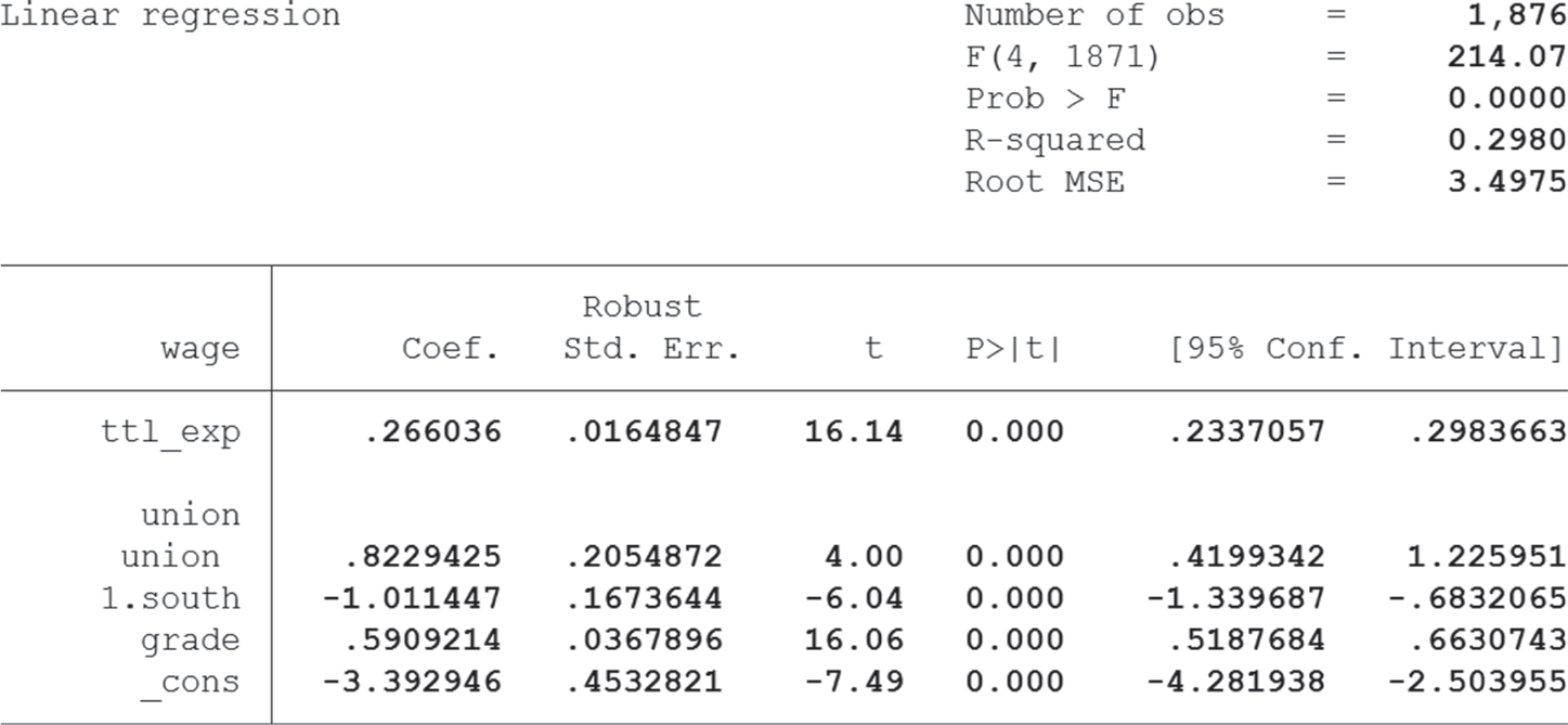
You will notice that the coefficients are identical to the normal regression, but the standard errors and, therefore, also the confidence intervals changed slightly. You can compare the results to the same model which uses regular standard errors (see page 92). To summarize it, you can use robust standard errors when you expect high heteroscedasticity but keep in mind that they are not magic and when your model is highly misspecified they will not save your results. Some statisticians recommend to calculate normal and robust standard errors and compare results: if the difference is large the model is probably poorly specified and should be revised carefully (King and Roberts, 2015). So you see, this option can be helpful in some cases, but sometimes it will not yield the best outcomes.

If you come to the conclusion that robust standard errors will not really improve your model, you can transform your dependent variable, as described above, and later re-transform the predictions to produce results that can be interpreted easily. We will choose a log-transformation for the example (make sure you have created the logged variable as explained before):

quietly regress lwage c.ttl_exp i.union i.south c.grade
margins union, at(ttl_exp=(0(4)24)) expression(exp(predict(xb)))
marginsplot

The magic happens in the option expression. We specify that the exponential-function (exp) should be applied to the result, as this is the inverse-function of the log-function. Finally, Stata produces a nice graph for us which shows the effect of union-membership for certain values of work experience. This method is not restricted to the log-function, as long as you specify the correct inverse-function for re-transformation. Note that this is an advanced topic and you should further research the literature, as the “best” transformation, or method, also depends on your research question and your variables. For example, some statisticians even prefer a poisson model over the regression with a log-transformed variable.54

7.6.1 Dfbetas

The first option for checking special cases are Dfbetas. Run your regression model as usual and type

dfbeta

or click Statistics → Linear models and related → Regression diagnostics → DFBETAs, name the new variable and click Submit.

Stata creates four new variables (one for each metric or binary variable and one for each category of a categorical variable). You can get a nice visualization by typing

scatter _dfbeta_1 idcode, mlabel(idcode)

The further the absolute distance of a value from zero the greater the influence. You can check the cases which seem the most distant and inspect them individually. Then repeat for all other created dfbetas. There is a rule of thumb to estimate the value above which cases are problematic, which is calculated by the formula$\frac{2}{\sqrt{\left(n\right)}}$ , where n is the number of cases (observations) used in the model. In our example this would be$\frac{2}{\sqrt{\left(1876\right)}}=0.0462$

We can get a complete list of all cases that violate this limit by typing

list if abs(_dfbeta_1) > 0.0462 & !missing(_dfbeta_1)
count if abs(_dfbeta_1) > 0.0462 & !missing(_dfbeta_1)

- output omitted -

Do not forget to exclude cases with missing values, as otherwise these will be listed as well!

According to this, 83 cases are problematic (this is the result for the first dfbeta only). As there is no general rule for dealing with these cases, it is up to you to inspect and decide. When you do nothing and just ignore influential observations, it is also fine, as these are rarely discussed in research papers. When you are unsure what to do, consult your advisor (as he or she is the one who will grade your paper).

7.6.2 Cook’s distance

When you do not like Dfbetas, since they are tedious to check when you use a great number of variables in your model, an alternative is Cook’s distance which summarizes all information in just one variable. This measurement detects strange patterns and unusual variable constellations and can help to identify coding errors or problematic cases. As usual, run your model first and type

predict cook, cooksd
scatter cook idcode, mlabel(idcode)

or click Statistics → Linear models and related → Regression diagnostics → Cook’s distance, name the new variable and click Submit.

You can now inspect the scatterplot visually and have a look at the problematic cases that have unusually large values. One example is clearly case number 856, so we will list the relevant information for that particular observation.

list wage ttl_exp union south grade if idcode == 856

This person has an extraordinarily high income, although her education is only medium and she is from the south. In general, this is a strange constellation which causes the high leverage of this case on the results.

A final possibility is to use leverage-versus-squared-residual plots which combine information about the leverage and residuals. This makes detection of outliers easy. Just run your regression and type

lvr2plot, mlabel(idcode)

This plot shows for each case, the individual leverage (y-axis) and residual (x-axis). If the residual of a case is high, this tells us that our model makes a prediction that is quite off from the real outcome. Therefore, the residual is related to the dependent variable of the case. A high leverage of a case tells us that the constellations of independent variables of a certain case are so extreme, or uncommon, that they influence our final result over proportionally. Therefore, the leverage is related to the independent variables of a case. The two dotted lines in the graph show the means for both residuals and leverages. The diagnostics reported here are not exhaustive, as a much longer list of tests and method exists that can be used to assess the results of a regression. By listing the most important aspects that you should always control, I think that the results should be quite robust and suitable for publication. It is always a good idea to ask the people who will later receive your paper whether they have extra suggestions for tests that you should apply. Also, have a look at the literature and footnotes throughout the chapter, as they provide ­valuable information.