Systems of Cities and Inter-City Trade

J. VERNON HENDERSON

Brown University, Providence, RI, USA

This chapter examines the role of cities in an economy. What do cities produce, when do they specialize in industrial production and when are they diversified? Why are cities of different sizes and what are the forces determining city sizes? How do cities interact with each other? What are the determinants of urban concentration, in terms of whether population is located in larger versus smaller types of cities? What are the impacts of government policies on urban concentration and urban development? What are the impacts of natural resources, economic growth, and international trade on a system of cities? What are the determinants of population composition of cities, in terms of high versus low skill workers? Are the patterns which evolve in a free market economy efficient ones, or are there externalities or incompleteness of markets which deter the realization of efficient outcomes?

Over the last decade or so, there has been extensive work on developing a model to analyze the positive questions (Henderson, 1972, 1974, 1982a, 1982b), Henderson and Ioannides (1981), Hochman (1977, 1981), Kanemoto (1978, 1980), Upton (1981) and Miyao (1981), as well as extensive work on the normative issues (Mirrlees (1972), Flatters, Henderson, and Mieszkowski (1974), Henderson (1977), Stiglitz (1977), Arnott (1979), Arnott and Stiglitz (1979), and Hochman (1981). This chapter is divided into two parts, a long part examining the positive issues and a shorter part examining the normative issues. The strategy of presentation is to summarize the basic models and theoretical results in the literature, to summarize the debates and unanswered questions concerning the assumptions and limitations of these basic models, and to summarize the conclusions of selected empirical work which gives answers to some of the debated issues. There is also an emphasis on pointing out directions for future work.

PART ONE – POSITIVE ANALYSES

1. Cities and the structure of the economy

1.1. Conceptual notions

Early models of systems of cities conceived of cities as primarily serving a rural agricultural sector. In Lösch’s (1954) framework, urban firms export all production to a uniformly distributed agricultural population where the market area for each producer of each type of good increases with the degree of scale economies in production of the particular good and decreases with the particular costs of transporting the good to farmers. Given the notions that traditional towns serve agriculturally based populations but that market areas vary by the type of good produced, central place theory as exposited by Beckmann (1958) postulates a hierarchy of cities (see also Christaller (1966)).

The formalization of traditional hierarchy models depends on three critical assumptions. First, there is a parameter k which describes the number of people in a city required to serve a given population (including itself), with unspecified products. If p_n is the population of an nth order city and P_n the population served by that city, then p_n = kP_n. Second, the smallest size city of order 1, serves an exogenously given rural population r, so that P₁ = r + p₁. Combining the first two assumptions we have that p₁ = kr/(1 – k) and p₁ = r/(1–k). Finally, there is an assumption that each city serves s cities of the next smallest size so that P_n = p_n + sP_n–1. If we solve the system of equations (e.g., Mills (1972)) we get that

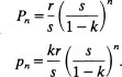
This yields the interesting property that the population of higher order cities increases exponentially with rank. We can also manipulate the relationships to generate the rank size rule (see later).

The obvious questions about this type of formalization are three-fold. First, the parameters s, k, and r implicitly must reflect underlying demand, supply and transportation conditions. However, there is no role for prices or possibilities for normal comparative static analyses in the model. Second, the goods produced by cities are not formally in the model. Parr (1969) does have a formulation where cities export goods down the hierarchy, there are as many goods as ranks of cities and each city produces the goods of its and lower order ranks. He then allows a k specific to each type of good. Specifying trade to only occur down the hierarchy leaves the question of how cities balance their trade, or what goods the highest order cities import. The final question is what happens in an industrial region if there is no agricultural population to base the analysis on.

Beckmann’s model provides a benchmark, for what we think might be reasonable predictions about systems of cities. The task is to define a model where the existence of a system of cities is compatible with, but not dependent on, the existence of a nation-wide agricultural sector, where the internal structure of cities is accounted for, and where demand and supply technologies, markets, and prices appear explicitly so that comparative statics and dynamics are possible.

In a classic paper, Mills (1967) suggested that cities form in an economy because there are scale economies in industrial production which lead workers and firms to cluster together in large agglomerations, rather than dispersing more or less evenly over the geographic area of the economy (with or without an agricultural sector). The scale economies are dependent on workers and firms working together in close spatial proximity in, for example, a Central Business District [CBD] of a city and apply to the production of goods which are exported from the city to other cities or economies. Greater scale of economic activities in cities enhances productivity through “communications” among firms which enhance the speed of adoption of new technological innovations and of reaction to changing national and international market conditions, through labor market economies for workers and firms searching respectively for specific jobs and specific skill combinations, through greater opportunities for specialization in firm (and worker) activities, and through scale economies in provision of intermediate common inputs (docking facilities, warehousing, power, etc.).

At the same time, there are consumption and certain production diseconomies connected with people clustering together in urban areas, such as commuting cost increases in a monocentric city, and such disamenities as crime, pollution, and social conflict. In a monocentric city where almost all residents work in a Central Businesss District, as city size expands, residents on average live further and further from the city center and have to commute greater and greater distances. The effect of these diseconomies will be to eventually offset production scale benefits as a city’s size increases, limiting cities to various equilibrium sizes (Mills (1967) and Dixit (1973)).

Given cities exist and are limited in efficient sizes, how do they relate to each other? One basic notion here is that there are different types of cities, where each type specializes in the production of a different traded good. Then each type of city trades with every other type. The extent of specialization of cities is, of course, limited. There are a range of goods produced in almost all urban areas—general retailing, schooling, housing services, auto repairs, dry cleaning, etc. These services as well as some manufactured goods are nontraded simply because the transport costs of intercity trade are prohibitive.

This implicit introduction of transport cost considerations is a recurring phenomenon throughout the systems of cities models. As will become clear, a basic lacking of the models is the explicit modeling of transport cost considerations. Unfortunately, such modeling is extremely difficult to do mathematically in any generalized fashion. We will comment more on this.

Scale economies and specialization. We will argue that notions of specialization and the nature of scale economies are closely linked. However, before examining these links it is useful to examine the extent and form of specialization. Specialization in the U.S.A. seems to be pervasive amongst smaller and medium size urban areas (Bergsman, et al., 1972, 1975), where about half of the 243 U.S.A. SMSA’s in 1970 Henderson (1986b) could be classified as being specialized in one of auto production, aircraft, shipbuilding, steel, industrial machinery, communication equipment, petrochemicals, textiles, apparel, leather products, pulp and paper, food processing. The other half of the SMSA’s are either non-industrialized state capitals, college towns, and agriculture service centers (specialized in warehousing, business, and transport services) or very large diversified metropolitan areas. As another example, for Brazil the pattern is similar, although not surprisingly, there are relatively more urban areas specialized in textiles and food processing and relatively fewer in transport equipment, machinery, and petrochemicals.

It should be noted that specialization in this context is very much a relative concept. Much of a city’s labor force is engaged in non-export service and retail activity. At most 40% of a city’s labor force will be engaged in one type of export activity. Typically specialization is defined on the basis of 10–20% of the city’s labor force being engaged in one particular manufacturing or service activity, with perhaps another 10–20% being involved in diverse other activities, with many support activities for the industry of specialization. Other patterns are possible. For example, an industry typically employing males (iron and steel) is sometimes complemented by an industry likely to employ females (textiles).

Specialization can also be viewed from another perspective. In Brazil for most three- and four-digit manufacturing industries, in looking at any one of these industries, there appear to be three sets of urbans. The first set containing typically well over 50% of all urban areas has absolutely no employment in that industry. The second set containing typically 35–45% of all urban areas has minimal employment (under 150 workers) in that industry, typically involved in repair and service activities. The final set containing typically 5–10% of all urban areas has extensive employment in that industry, with that industry often being its industry of specialization.

The discussion of specialization so far applies most directly to smaller and medium size urban areas. It appears (Bergsman, et al. (1975) and Henderson (1986b) that, while the very largest metropolitan areas do exhibit some tendency towards specialization, some large part of their work force is found in a whole spectrum of industrial classifications, unlike smaller urban areas. That evidence may not be inconsistent with the notion of specialization. Given the above discussion, specialization occurs primarily at the level of a monocentric city contained in a single political jurisdiction, a description that could be given of a smaller urban area. However, a very large metropolitan area may contain several or many specialized industrial centers surrounded by the residences of their work force and governed independently in a jurisdictionally fragmented metropolitan area. In short, a large metropolitan area may contain a number of “cities” that could exist on their own, a notion that is further developed later.

Having established the fact of some extensive degree of specialization, we must ask why it occurs. There are strong forces against specialization—the intercity transport costs of trading good, the intercity costs of transporting intermediate inputs in production, and diversification for a city in the composition of its industrial output to insure against the risk of secular and/or cyclical changes in the demand for individual industrial products.

Several reasons can be given for specialization, such as site specific extractions of different raw materials or Tiebout forces encouraging population stratification for consumption purposes resulting in different skill compositions and hence comparative advantages of different cities (Berglas (1976)). Site specific extraction is a very limiting factor in a model, given extraction and processing is typically a small part of national output, and does not imply specialization per se, just that one of the products locally produced will be resource intensive. Tiebout type stratification in the U.S.A. across urban areas appears to be almost non-existent, as measured by education, income, and age characteristics (Getz and Huang (1978) and Henderson (1982c)). To the extent age and education varies across cities it appears to be explained by skill demands of industries and youth migration from declining regions.

An alternative explanation of specialization is based on the nature of scale economies. Henderson (1972, 1974) argues that specialization occurs if there are no production benefits or positive externalities from locating two different industries in the same place. If they are located together, because workers in both industries are living and commuting in the same city, this raises the spatial area of the city and average commuting costs for a given degree of scale economy exploitation in any one industry. Separating the industries into different cities allows for a greater degree of scale economy exploitation in each industry relative to a given level of commuting costs and city spatial area.

This argument concerning scale economies is strengthened if scale economies are ones of localization, not urbanization. Localization economies are ones internal to each industry, where scale is measured by total employment (or output) in that industry in that urban area. Urbanization economies are external to the specific industry, and result from the level of all economic activity internal to a city, measured by, say, total city population. In this case, only the size of the city, not its industry composition, affects the extent of scale effects relevant to a particular industry.

If scale effects are ones of localization, then for a given city size and associated cost of living, scale effects and hence incomes are maximized by concentrating local export employment all in one industry, rather than dissipating the scale effects by spreading employment over many industries. However, if scale effects are ones of urbanization, then this specialization may not matter since it is the general level of economic activity rather than its industry specific concentration which enhances productivity. However, it should be noted that, if industries have different degrees of urbanization economies, specialization could occur under urbanization economies because the most efficient size of a city for each industry would differ by type of industry (see later). This is a much weaker force for specialization than localization economies, to be weighted against the disadvantages of specialization (transport costs of trade, lack of industrial diversification for insurance). Again, however, transport cost considerations are brought in the back door of the model.

There is some debate in the empirical literature about the nature of scale economies. Some older literature (Shefer (1973), Carlino (1978)) results in a very restrictive interpretation of a CES production function. More recent approaches implicitly (Sveikauskas, 1975, 1978) or explicitly (Henderson, 1986a, 1986b) use a flexible functional form approach to specifying technology. In comparative testing for Brazil (Henderson, 1986a, 1986b) and the U.S.A. (Sveikauskas (1978, Table 9), Henderson (1986b)), localization economies rather than urbanization ones appear to dominate for industries such as primary metals, electrical and non-electrical machinery, transport equipment, petrochemicals, pulp and paper, leather products and wood products. The extent of localization economics for apparel and textiles in both countries and food processing in Brazil is weaker suggesting weak benefits from agglomerating employment in these industries as opposed to their being in small towns (rural areas). These industries exhibiting localization economies tend to produce standardized products that are exported from the city nationally and internationally. Because the products are standardized it is not so important for them to be in centers of innovation. Rather they benefit from either or both large plant sizes with large assembly lines (e.g., transport equipment) or from large own industry concentration drawing upon a common labor market (e.g., pulp and paper, wood products, textiles).

In contrast, ubiquitous industries where many products are locally consumed such as (fabricated metals (e.g., cans, cutlery, hand tools, plumbing fixtures, structure of metal products, stampings) and non-metallic minerals (e.g., cement, glass) exhibit little or no scale effects. And volatile consumer oriented industries such as apparel and publishing appear to benefit more from increases in urban area sizes, than own industry size per se. There were few robust patterns of industry productivity being affected by employment in related industries as defined either by input-output connections (forward and backward linkages) or correlations in spatial patterns.

Given these notions that an economy consists of a system of cities of limited efficient sizes, where there are different types specialized in different activities, we can now turn to a formal model of a system of cities. Before examining the system, we must develop a model of a single city and then work up from there.

1.2. Model of a single city

In order to analyze the positive characteristics of a system of cities, the model of a single city must be chosen carefully. In the literature it is typical to use a specific functional form model, without explicit spatial dimensions. There are three reasons for this choice of modeling strategy. A sophisticated spatial model of a single city is too cumbersome to develop the properties of a system of cities within a paper of acceptable length and exposition and that level of detail for a single city adds little or nothing to the analysis of the properties of a system of cities. In fact, it generally takes a whole paper to develop the properties of a single city if a spatial model is used (e.g., Dixit (1973) or Wheaton (1974)). The only exception is a fixed lot size model (see Henderson, 1977, Ch. 3), but that model does not permit substitution in production and consumption of housing and does not permit any ready modeling of urban infrastructure—as we will see these are distinct disadvantages. Second, specific functional forms are used in part, because for certain propositions concerning city size distributions closed form solutions are highly desirable. Finally, specific functional forms are generally chosen over general functional forms because when general functional forms are used in this type of complex model with scale (dis)economies, in developing propositions through comparative statics, various output elasticities with respect to inputs are defined and propositions can only be proved with these elasticities treated as global constants (e.g., Hochman (1977). It is not clear it is an improvement to implicitly introduce specific functional forms at the point of proving propositions, relative to defining specific functional forms up front to begin with.

These comments do not apply to models of the normative characteristics of a system of cities. Such analyses as described in Part 2 of the chapter utilize a general functional form spatial model (Henderson (1977, 1977a), Arnott (1979), Arnott and Stiglitz (1979), Kanemoto (1976)). In normative analyses the land rents generated in a spatial model as we will see play a critical role. They can also play an important role in positive analyses, which in the context of a nonspatial model requires reference to their existence.

The model of a single city typically consists of three components—the production sector, consumption sector, and the local government sector. We start with the production sector.

Production. Two final outputs are produced in each city. One is the traded good the city specialize in, which is produced with capital and labor under constant returns to scale at the firm level. Firms are subject to a Hicks’ neutral shift factor, where increasing industry employment results in increased industry efficiency for all firms. Since such economies of scale are external to the firm, perfect competition and exhaustion of firm revenue by factor payments prevail (Chipman (1970)). The efficiency implications of the externality will be dealt with later in the paper. Under the specification we may use the industry production function

X, ₀, and ₀ are respectively industry output, labor inputs, and capital stock. g(N) is the shift factor, where N is the number of city residents (who divide their time between X production and commuting). The specification of g(N) presumes specialization in X production and would not prior to specialization include residents employed in and commuting to other industries, given we are assuming economies of scale are localization ones. The form of g(N) will be discussed below, although we assume positive scale economies so g′ > 0.

Not all authors utilize this formulation of industry scale economies. Some (e.g., Mills (1967)) assume scale economies are internal to the firm, which implies in each city in equilibrium there can only be one firm in the traded good sector, who is thus a local monopolist. This model of a “company” town has the disadvantage of not corresponding to the nature of most cities in modern economies and can complicate the analyses of cities by forcing on them a monopolistic industrial structure—which raises a separate set of issues.

The second good produced in the city is a nontraded good, housing. In one formulation housing is produced with capital and ‘land’ sites under constant returns to scale; and the industry production function is

l are land sites produced with time, or labor, inputs subject to shift factors; or

₂ represents total labor resources, or time by residents, devoted to commuting in the city for a given number of residents (N) and public capital inputs (₂). Thus ₂ indicates the amount of land on the flat featureless plain ‘claimed’ through commuting by a given number of residents. N^–δ represents a spatial complexity factor. If, say, both ₂ and N double, land sites do not double because, in a spatial world, the new people located on the city edge must spend more time on average getting from their home site to work and back (in a monocentric model) and hence site production is less efficient. Proceeds from site sales (‘rents’) are exhausted by payments to ₂ (i.e., rents are distributed within the city). This ‘as if’ model of a spatial world is discussed extensively in Henderson (1972, 1974).

₂ represents public investment in transport facilities (roads) which reduces commuting time needed to produce sites. Note that the introduction of a public sector providing public capital is critical to the understanding of cities. Almost half the space of a city is public capital (including roads and sidewalks). In a growth context, a city cannot form and grow until much of its non-malleable public capital has been laid out. In general (in)efficient operation of local governments in providing infrastructure critically affects the sizes of cities, as we will discuss later. Unfortunately, many systems of cities models as well as single city models overlook this aspect of cities.

The breakdown of housing into housing (equation (2)) and site (equation (3)) production is not critical, and this complexity is avoided by some authors so that equations (2) and (3) are collapsed into one equation. For example, Hochman (1977) has housing only, which is produced with capital and labor subject to industry decreasing scale economies. He does not include public urban infrastructure, but his analysis could easily be amended to incorporate that.

Finally, there are on the production side, full employment equations for each city where

In the context of a system of cities the dynamics of labor market adjustment within and across cities to shocks to the system has not been considered. The only adjustment process analyzed concerns the abandonment and reclamation of immobile, non-malleable urban infrastructure in a growth situation, something we briefly discuss later.

Consumption. It is typical to assume residents have log linear utility functions of the form where we define are traded goods, one of which is produced by this type of city and exported and the others imported; and h is housing consumption. Normally it is easiest to work with the indirect utility function

where q_j are traded good prices, p is the price of housing and y is income. Typically, individuals derive income from wage payments and pay equal per person taxes to finance public transport expenditures. Thus

y is income, and r₂/N are local taxes financing ₂. This formulation of the system of cities model assumes capital rentals are distributed to capital owners outside the cities or outside the country, so that they are not spent on urban housing. The algebraically more complciated case, where capital rentals are spent in cities is also considered in Henderson (1972, 1974, 1982b) and Hochman (1977). The distinction can be important in examining the determination of city sizes and in examining regional factor movements. However, the basic propositions about a system of cities are unaffected by where capital rentals get spent.

The local government. A local government is introduced to determine the level of public investment ₂. In the context of a competitive, costless political process, it is assumed competing potential and incumbent governments seek to maximize the welfare of fully informed voter-residents so as to be re-elected. Given the fixed rental price of capital in national markets, for any city population, the government chooses ₂ to maximize U in (5), where the costs of increased taxes from raising ₂ are traded off against benefits of reduced land site and housing costs. The impact of having inefficient or non-autonomous local governments will be analyzed later.

To solve the model for the basic equations for a single city requires deriving marginal productivity conditions in production, substituting them into the housing demand equals supply condition and then doing further substitutions into the original equations (l)–(7). The results for our example (see Henderson (1982b)) for four critical equations are

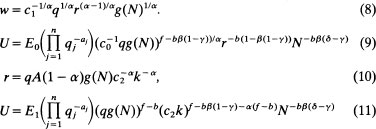
c₁ c₂, E₀, and E₁ are constants. Regularity conditions (positive capital rental rates and city sizes) require δ > γ f – bβ(1 – γ) – α(f – b) > 0 by definition.

In equation (8) w is the wage rate, q the price of X, r the rental on capital, and N city population. For one city of many in the economy facing fixed traded and capital good prices, wages rise indefinitely as city size increases. However, for utility in equation (9) while there are positive impacts on utility through wage effects there are negative cost of living effects through housing prices Before discussing equations (10) and (11), we examine the competitive determination of city size which is based on the wage-cost-of-living tradeoffs in equation (9).

City size. There are several equivalent ways to solve for city size. Henderson (1977) proves in a general equilibrium context, the only stable solution corresponds to one where, at the local level, ∂U/∂N = 0 (given identical technologies, traded and capital good prices, and amenities (see later) across cities). Any other potential solution to city size dissolves through factor flows, if one city in the system expands or contracts from the potential size through random factor movements.

Alternatively this size may be obtained through the direct actions of economic agents, such as competitive land developers who may set up cities in a national economy. These developers earn temporary profits in inefficient solutions by setting up and selling lots in cities of more efficient sizes than current cities. Note the implicit introduction of land rents (and hence space) in the last statement. Developers play an entrepreneurial role which facilitates large movements of people, so that a new city can form en masse, without having to wait until one individual alone would gain by moving to a new city (with others then following). Finally, ∂U/∂N = 0 could be achieved by local governments limiting city size to this utility-maximizing level, through a set of zoning ordinances. ∂U/∂N = 0 is always solved competitively under the assumption that a city faces fixed capital rental and traded good prices, or that it is one of many cities producing its export good and borrowing in capital markets.

To solve ∂U/∂N = 0 for the efficient N, we must specify the nature of the external localization economies function g(N). To do so, we borrow from the econometric literature on the nature of localization economies. Looking at both two- and three-digit industries for the U.S.A. and Brazil, Henderson (1986b) finds that for almost all industries a declining elasticity ((dg/dN)/(g/N)) formulation dominates a constant (or increasing) elasticity formulation. The easiest form to work with econometrically is

where (dg/dN)/(g/N) = ϕ/N > 0. This is the form we use in this presentation.

Apart from the empirical justification, it is critical in the overall model to break the logarithmic linearity of the system of equations so as to get unique, non-infinitesimal and non-infinite, efficient city sizes. This can be done either by having the degree of scale economies peter out, so the agglomeration benefit of increasing city size dies out, by having the degree of diseconomies in land site production escalate (i.e., increasing congestion) so urban costs of living escalate with city size increases (Henderson (1974)), by having city size itself be an increasing disamenity in the utility function (Henderson (1982a, 1982b)), as well as other ways (Upton (1981), Henderson (1977)).

Substituting in (9) for g(N) and solving ∂U/∂N = 0 we get efficient city size is

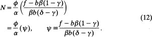
ψ is a parameter which summarizes the internal structure of cities, excluding the export sector. Thus it is common across city types. Existence of positive city sizes and satisfaction of second order conditions together require is a common parameter collection throughout the paper, so we redefine it as ψ. Note in (12), if consumers’ taste parameter for housing b/f rises, if the land intensity of housing production β rises, or if spatial complexity parameter δ rises, efficient city sizes fall. All of these factors lead to greater increases in costs of living as a city’s size expands. Either more land is utilized by consumers increasing commuting distances or commuting becomes more costly. Finally, if the productivity of infrastructure investments, γ, rises, efficient city sizes rise since costs of living rise more slowly. Other properties of (12) will be noted later.

Underlying equation (12) in a general equilibrium context is a tradeoff between the gains to capital owners versus the losses to laborers of increasing city size beyond some point. This can be seen by examining equations (10) and (11) for capital rentals (r) and utility levels defined in terms of the capital to labor ratio, k. Assume for illustrative purposes a one sector economy with just one type of city (but many cities of that type). Normalize q at 1 and note that a stable equilibrium solution (Henderson, 1972, 1974) will require all cities to have the same k, which hence equals the national k. For a constant k in equation (8), U rises with N until

and then declines. First, note

given f – bβ(1 – γ) > f – b. Second, r in equation (11) rises indefinitely with city size. The equilibrium N in equation (12) represents the point in a general equilibrium context for a fixed k, where

or the marginal losses to laborers in monetary terms from increasing equilibrium city sizes just equal the marginal gains to capital owners. In a competitive market economy this solution is realized by competitive cities maximizing U in equation (9) in a “partial” equilibrium context for r and q (but not k) viewed as being exogenously given.

However, it should be recognized that capital owners would benefit at the expense of laborers if city sizes were all forced beyond their equilibrium levels. Capital owners would gain because unlike laborers they are not bound to live in the city where their resources are employed, and endure high costs of living. While an economist would normally view this notion as a curiosity which has no relevance to realized competitive outcomes, those who view the world as a conflict between laborers and capitalists can get quite excited about the possibilities inherent in collusive action.

2. Basic properties of a system of cities

2.1. General equilibrium properties

Using the model of a single city we can solve for the characteristics of equilibrium in a system composed of multiple types of cities. To do so requires looking at equilibrium in national markets given equilibrium conditions in individual cities. It is typical to assume capital and labor are perfectly mobile within the economy, although the economy could be divided into regions between which labor is imperfectly mobile. At this point subscripting is introduced, where etc. refer to values of parameters and variables for the jth type of city, specialized in the export production of X_j. We compare the jth type of city with the first type, where q₁ = 1 is chosen as the numeraire. The parameters of housing and site production and all utility functions are the same across cities. Only the production sector differs. There are n types of cities. We first examine how city size, wages, capital rentals and capital usage vary across types of cities.

Variations in sizes across city types. First, re-examining the city size equation we see that

where ψ in (12′) is common to all cities. Thus comparing different types of cities, N_j is a linear function of ϕ_j/α_j, where ∂N/∂Nϕ > 0, ∂N/∂α < 0. City sizes increase with the degree of scale economies which indicate a city’s ability to pay higher wages for a given capital rental. Sizes also increase with capital intensity in production, where increased capital intensity means that a city can support a given wage-capital rental ratio with less population and a lower cost of living. As ϕ/α→0, city size becomes negligible. We could think of goods with low levels of scale (ϕ) as being rural or agricultural products, where our “city” becomes a family farm or small village. That is, there is nothing in the model which limits the inclusion of an agricultural sector, defined as the smallest type of “city”, although this obviously overlooks the explicit spatial aspects of the problem.

It is also easy to see the difficulties in moving to general functional forms from specific functional forms by considering equation (12’) and its derivation. ϕ and α are global parameters. In a general functional form context they should be parameters defined at the margin. Without knowing intra-marginal movements of ϕ and α, one could not conclude that ∂N/∂ϕ > 0 or ∂N/∂α < 0. Worse, without globally restricting ϕ and α, we cannot conclude that U(.) in equation (9) has a single maximum point with respect to N or that it has a maximum point at all. In short, without imposing a number of strong assumptions on the general functional form model one cannot proceed as we are doing. The assumptions made in the literature about functional forms are made for this reason.

Variations in prices across city types. To solve for the other properties of a system of cities involves examining equilibrium conditions in national labor, capital, and output markets. For labor market equilibrium, between any pairs of cities, laborers must be equally well off so that they do not move. Therefore, U_i = U₁ and from (9) solving out for q_j we get

This is a key equation in solving inter-city equilibrium. First, by substituting back into wage (equation (8)) and housing price equations we can show that

Given ψ > 0, equation (14) unambiguously states that in comparing types of cities both wages and housing prices are greater as the size of cities rise across city types, for equal utility levels across cities. The point of course is intuitive. Wages and cost-of-living rise with city size because respectively scale economy benefits are greater and commuting distances and the corresponding housing costs are greater. To maintain equal utility across cities, in the absence of other considerations, they must each rise by the same percentage, as city size increases.

The fact that wages and costs-of-living rise with city size is documented empirically in the numerous wage-amenity studies (e.g., Rosen (1978), Izraeli (1979), Getz and Huang (1978), Hoch (1977)). However, the magnitude of wage increases is much greater than might be anticipated for “expected” magnitudes of ψ = (f – bβ(1 – γ))/(δ – γ)bβ) (e.g., b/f = 0.2, β = 0.15, (γ – δ) < 0.5), a reflection of the simplicity of the model and perhaps the assumption of efficient urban infrastructure provision. For example, for Southern Brazil Henderson (1986a) estimates that, controlling for skill levels and amenities, wages of workers must rise by 0.66% for each 1% increase in urban area population to maintain the same consumer standard-of-living. Thus in Brazil over the relevant size range of urban areas, in moving from populations of under 50, 000 to ones over 200, 000, wages more than double and in moving from medium size cities to large metropolitan areas wages rise by another 50% or so. For example, in a sample of 109 Southern Brazilian cities ranging in size from about 10, 000 to 10 m, wages for urban low-skill workers were 3.1 times higher in Sao Paulo compared to the smallest cities (population of 10, 000). This is not incompatable with estimates of cost-of-living increases between rural and urban areas in Peru (Thomas (1978)).

There are also certain implications for capital intensity in production of these price variations. Given capital rentals are constant across cities, housing prices rise because “land site” costs rise. Given this we would expect to see the use of capital relative to “land” rise in housing production as city size increases. Secondly, we would expect as housing prices rise, consumption of housing relative to other goods falls. Finally, we would expect efficient relative urban infrastructure investment levels to rise. In the current model this can be shown by examining how the per capita usage of capital in housing consumption, and per capita infrastructure investments vary with city size. For example, it can be shown that for a given r

That is, as N_j rises relative to N₁ the per capita usage of and in j type cities rises relative to 1 type cities. The taller buildings, smaller floor spaces, and greater complexes of intra-city freeways of larger cities are casual evidence that these phenomena occur.

Variations in capital usage. While capital usage in urban infrastructure and housing tends to rise with city size, it may not be the case that overall capital usage including the production sector rises with city size. Hochman (1977) first pointed out how important it is to analyze how capital usage varies across city types. From national capital market equilibrium, r_j = r₁. Equating r_j, and r₁ in equation (10) and substituting in for q_j from (1) yields

By straight differentiation after substituting in (10) it can be shown that

A city’s capital usage increases as scale economies and capital intensity in export production increase. That is, for ϕ_j = ϕ₁[α_j = α₁], k_j > k₁ if α_j < α₁[ϕ_j > ϕ₁] However, neither α_j < α₁ N_j > N₁ necessarily imply k_j > k₁

This distinction between the overall capital usage of a city (including capital usage in housing and social overhead capital) and capital intensity in production of the city’s good is critical. Potentially, capital intensive goods can be produced in high labor usage cities. A sufficient condition for the type j city to have relatively high capital usage (k_j > k₁ is that both X_j be relatively capital intensive (α_j < α₁) and the jth type city be larger (ϕ_j/α_j > ϕ₁/α₁). However, even if α_j < α₁, k₁ can exceed k_j if ϕ₁/α₁ > ϕ_j/α_j and type 1 cities are larger, hence have higher wage costs, and thus spend more per capita on capital in housing and public transportation. As we will discuss later, if k₁ > k_j when α₁ > α_j the stability of equilibrium comes into question (Hochman, 1977) and economies will tend to completely specialize if they engage in international trade (Henderson, 1982b).

2.2. Urban concentration

The numbers of cities by size and type. To solve for the ratio of numbers of each type of city, denoted by m_j, we equate national demand and supply for each type of good. National supply is m_jX_j, National demand, providing all people have the same logarithmic linear utility functions is where I is national income net of local taxes. Thus for any two types of cities

If we substitute in this expression for X_j, X₁ and q_j we get

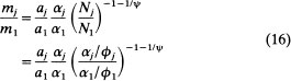
m_j/m₁ increases as a_j/a₁ (relative demand for X_j) increases, and as α_j/α₁ increases or ϕ_i/ϕ₁ declines and hence N_j/N₁ declines. The latter result simply indicates that the same relative amount of X_j would be produced in more but smaller cities.

In solving equation (16) we have assumed a “large” enough economy so that when the population is divided into the integer number of optimal size cities, any problems with remainders are negligible. This means any remainders are divided amongst so large a number of cities, that their impact on individual city sizes is negligible. This problem is analyzed in detail in Henderson (1972, 1974) and is discussed in Part 2.

From equations (12) and (16) for city sizes and numbers, it should be clear that the sizes and numbers of each type of city reflect underlying demand and supply conditions in the economy. Moreover, any regularities in the patterns of cities and their size distribution, such as the geometric series or rank size rules, imply very specific demand and supply conditions and national output patterns. The rank size rule says that if we rank all cities by size with the largest having rank 1 and the nth largest rank n, rank multiplied by size is approximately constant over all cities. Such a relationship has been observed at least casually in various regions and countries although one should not treat it as a stylized fact we must explain. Allowing for some stochastic variation in city size (Mills, 1972), caused by, say, drawings of amenity bundles (see below), we can develop the implications of a rank size rule in our model, which will suggest how our parameters might be restricted to vary together as we moved across types of cities. Because so many parameters are involved the restrictions are weak.

However, it is important to note that in practice these theoretical links between city industrial specialization, city size, the size distribution of cities and national output patterns are rough. While in theory, city size is directly linked to internal industrial composition, in practice the link for a specific city is weak (Henderson, 1986a and 1986b). As we will argue, city size is strongly affected by consumption considerations and geographic characteristics such as (i) public service levels, qualities, and taxes; (ii) quality of life measures such as crime rates and pollution levels; (iii) natural amenities such as weather conditions which affect everything from heating costs, to health, to pollution dispersion; and (iv) geological formation affecting the city’s shape and transport system. In short, each city’s attributes are unique and its efficient size different. Moreover, both simple simulation work in theoretical models and econometric work indicates that small variations in the key characteristics of a city can produce large variations in city size without affecting the welfare of residents. References on this include (Tolley, et al. (1979), Yezer and Goldfarb (1982), Henderson (1986b), and Segal (1976)).

Second, it is true there is a relationship between the industrial composition of national output and the size distribution of cities which results because many smaller and medium size cities tend to specialize in industrial production and each type of city on average has a different size. However, it must be recognized that on an absolute basis much industrial production occurs in large metropolitan areas (e.g., Philadelphia, Chicago, Detroit, Newark in the U.S.A.) and that even some not so large metropolitan areas have diverse manufacturing bases (e.g., Buffalo, Phoenix, Syracuse, and Dallas in the U.S.A.). Part of this is historical where population has clustered around a resource based core city, a phenomenon we explore next. But much of it probably involves complex interrelationships between specific industries identified at a very detailed level (i.e., looking at four- or five-digit industries rather than two-or three-digit) which we have only just started to study (see Bergsman, et al. (1972) (1975)), and for which data is limited.

2.3. The impact of natural resources on urban concentration

The impact of natural resources on a system of cities is at a very preliminary stage of analysis in the literature. Here we outline two initial attempts to model natural resource impacts. Both attempts also point the way to how explicit modeling of inter-city transport costs of trade might eventually be handled. The first deals with competition amongst cities for urban sites with favorable amenity endowments. The second deals with modeling the spatial configurations of cities engaged in natural resource using production versus those engaged in footloose production. Neither model meets Beckmann’s (1968) call for a general analysis of spatial configurations of primary, intermediate, and final production.

The first approach concerns amenities, rather than raw material inputs. Geographic locations have different endowments of amenities which affect consumers and producers. Consumer amenities could be represented by a vector of attributes represented in the shift term, E, of the utility function. E could vary with an urban site’s climate, access to outdoor recreation alternatives, access to drinking water, and so on. Similarly, producer amenities could affect the value of the shift term, A_j, of the production function for each type of city. Such amenities could include natural harbors, access to fresh water, climate, elevation, etc. and their impact on the shift term could differ according to the type of good X_j being produced. It is also possible to model transport costs as a production function shift factor increasing the extent of “evaporation” of the product as access to national markets falls.

Upton (1981) and Haurin (1980) have modeled this type of situation for a single type of city. In our framework, the analysis models equilibrium among all cities of one type, say the jth type. Assume all possible urban sites in the economy have different amentity vectors. Favorable vectors increase the values of E and A_j which increase potential utility for a given city size. Thus looking at the jth type of cities, given they will be on different quality sites, they will have different utility paths. In our model, each path will have a maximum point at the same N_j but cities on better quality sites will have higher paths (at each city size), so that, with free entry, cities with better amenity vectors and higher utility paths will be larger.

In relative terms, the benefits of better amenity vectors will be dissipated by cities on better sites expanding until their cost-of-living increases drive their utility levels down to that prevailing nationally. In absolute terms, citizens in an economy with better selection of urban sites may be better off than citizens in an economy with inferior sites. However, within economy, utility levels cannot differ by urban site quality, given equilibrium in national labor markets.

Formally, modeling equilibrium when urban site qualities and city sizes of the same type differ is cumbersome (Upton (1981)) and has not been attempted for multiple types of cities. However, it does provide a basis for all cities in an economy being of somewhat different sizes even if they produce the same goods. We briefly speculate on how such a model could be extended to multiple types of cities. We focus on amenities which provide equal benefits to all types of cities, such as consumer amenities affecting the E shift factor. Then comparing different types of cities, it seems reasonable that in equilibrium larger types of cities would occupy better sites, so that the m₁ cities of type 1 would occupy the best m₁ sites, type 2 cities the next best m₂ sites, and so on. Why is this reasonable? In the way we have formulated the problem, the factors affecting the E’s are like public goods. Larger cities have more people to enjoy the public good benefits and thus are willing to pay more in total for amenities through, say, land rents in an explicit spatial model. Alternatively stated, larger cities have higher rent gradients and higher total urban rents. In competition they thus can pay more for sites of better quality and can bid them away from smaller types of cities.

The second way natural resources appear in a system of cities in the literature (Henderson, 1982b) is in an attempt to explain the phenomenon of metropolitan areas. Our discussion so far really relates to economies composed of cities that are essentially monocentric. Even today much of the urbanized population in most countries remains in cities that are primarily monocentric. In some countries, however, a significant portion of the urbanized population resides in large multinucleated metropolitan areas. We could interpret these areas as essentially being clusters of cities that would in other circumstances be spatially separate monocentric cities. Different types of cities could cluster together simply to reduce the transport costs of intercity trade among themselves. One limit on this clustering would be the need for cities to spatially disperse to utilize spatially dispersed resources.

To see the forces at work, we first consider the polar case opposite to the case where cities are all monocentric. Consider an economy composed only of metropolitan areas, where we treat metropolitan areas spatially as clusters of monocentric cities. A simple model that generates different size metropolitan areas and inter-metro area trade is as follows. Suppose some types of cities require the use of natural resources in production, while others do not. The natural resource locations are at various spots on the flat plain of the economy and the natural resources are very expensive to transport. Different types of cities using different types of resources would generally be spatially separated near different resources sites and would trade with each other across space.

In addition to natural resource using cities, there are a variety of other types of cities which are footloose. To reduce the costs of intercity trade these footloose cities cluster around the cities using site specific natural resources, to form multinucleated metropolitan areas composed of numerous different cities. Inter-metropolitan trade involves only natural resource products and metropolitan areas are self-sufficient in footloose products.

Suppose there are h type of footloose products produced and (only) sold locally, indexed by t. For a natural resource core city labelled i, equating demand and supply for each footloose industry we can solve for the numbers of footloose cities of type t

where |J_t| and |J₀| are parametrically given determinants. Metropolitan area size is then

Thus in this system of metropolitan areas, area population is an increasing function (at an increasing rate) of the base natural resource city population (N_i). If an economy produces relatively few footloose products and, say, fills its consumption gaps through international imports, then N_MA can be shown to be unambiguously smaller than in an economy producing more of its consumption of footloose products or even exporting them. Similarly ∣J_t∣/∣J₀∣ increases as the range of produced footloose goods rises with the numbers of existing types of footloose cities rising as well as the numbers of new types.

This modeling of metropolitan areas presents several problems. First, a “realistic” model would require a mixed model, with large metro areas based on a large type of natural resource core city producing a whole range of footloose products while smaller urban areas based on small types of core cities could not support production of many footloose industries. That is, the smallest cities perhaps could not consume the output of any local footloose industries, while intermediate size urban areas could only support production of a limited range of footloose products. Such a mixed model immediately introduces lumpiness problems in solving for footloose city sizes and in dividing up their output between local and export production. Again this is a cumbersome unsolved problem.

A second theoretical problem lies with the role of intermediate inputs and processing—with the all or nothing approach to defining whether an industry is natural resource based. The formulation certainly does not meet Beckmann’s (1968) call for a model depicting the role of cities in the sequence of extraction, processing, intermediate production, final good production, and retailing.

A third conceptual problem is that the extent of clustering despite the multinucleated specification does raise average commuting distances and land rents for all nuclei in the urban area. Metro areas are not in reality split into economically autonomous local communities. There is enormous cross commuting and the whole metro area typically functions as one giant labor market. Thus, for footloose industries which joint a metro area there must be certain urbanization benefits to help compensate for the higher land and wage costs. Completely standardized footloose production may then still locate in smaller and medium size specialized cities (e.g., textiles and appliances). Modeling the rise in land rent levels in a multinucleated urban area as the number of nuclei rises is still at an early stage.

Finally, there is the empirical issue of what should be the unit of observation in work on the nature of cities and production—the political unit of a city, the community, the urban area, the metropolitan statistical area, etc.? There is a very basic problem in defining and spatially interpreting what an urban or metropolitan area is. For example, there are several definitions of the New York urban area, starting from its five central boroughs and expanding west and north to incorporate outlying urbanized areas. The population range of these definitions goes from 7.5 million up to 18 million or even more. As New York City’s economy expanded historically, essentially its labor and housing markets overran other outlying previously independent urban areas. Thus, while the core urban area may be service and commerce oriented with also a market oriented apparel industry, as its economy overran outlying areas (such as Newark and Patterson) it has incorporated a diverse set of heavier manufacturing industries. The same problem exists in examining, for example, Chicago, Illinois. If we look at the core urban area versus its incorporation of parts of the state of Indiana, we get a different picture of its industrial base.

However, regardless of these problems, it should be apparent that the extent of urban concentration depends on the centralization and use of natural resources. If an economy has little in the way of fertile land and natural resources, its urban areas may be clustered around one or two ports which import its resources and export its products (e.g., Korea, with the national capital Seoul using Inchon as its port). On the other hand, if a country has rich inland deposits of iron, coal, forests, fertile land, and so on, it will have major inland metropolitan areas and sets of manufacturing and agricultural service cities (e.g., the U.K., Brazil and the U.S.A.).

2.4. Population composition of cities

So far we have assumed a world of identical inhabitants of cities. The formal introduction of two or more classes of people in a system of cities model has not been attempted. But theoretical work in two region model of an economy by Berglas (1976) and empirical work (Henderson, 1985, 1986a) suggest that this would be an important advance. In Berglas’s model there are two classes of people who have different demands for public goods and thus in a Tiebout context would prefer to stratify into the two different regions. However, production conditions require inputs of at least some of each type of worker in each industry. Thus stratification is imperfect. Henderson (1985, 1986a) estimates that for U.S.A. and Brazilian manufacturing industries high and low skill labor are either complements or poor substitutes in production, indicating that skill usage in production is a strongly limiting factor on the extent of stratification.

Moreover, the empirical work suggests that the consumer side of the model may be both complex and critical. First, it appears that high skill people have very particular public service demands (e.g., high quality educational facilities) and value the amenities of larger cities more than low skill people. This means particularly for a centralized system of government that to attract high skill workers to smaller cities requires good public service provision in these cities. Second, it appears low skill people view their high skill counterparts as an amenity, suggesting that low skill people are drawn to locations with relatively high concentrations of high skill people. This can present certain problems for stability in any model of this process, since the possibility of low skill people “chasing” high skill people exists.

2.5. The impact of government policies on urban concentration

A variety of governmental policies have far-reaching impacts on urban concentration and the system of cities. These include transport policies, capital market restrictions, restrictions on public service provision and local autonomy, minimum wage policies, and trade policies. Aspects of restrictions on local autonomy, minimum wage policies, and trade policies have been formally modeled in Henderson (1982a). In this section we discuss the potential impacts of various policies, utilizing formal analysis when it is available. Trade policies are discussed later.

Transport. A country’s transportation policies critically affect urban centralization and concentration. Obviously a country cannot effectively exploit its hinterland resources if it does not have an effective rail, water or highway trucking system to get the resources to producers and goods to national population centers and to ports for exports. But it is not simply a matter of resource exploitation. An effective transport system integrates an economy so that hinterlands can develop full systems of cities, producing lighter as well as heavier manufacturing products. It means that footloose producers can cluster near inland users of natural resources or sources of cheap power, labor and land and still have access to coastal and international markets. The critical role of transport development on decentralization in the U.S.A. has been studied systematically by economic historians (Fogel (1964)). However, to formally model these impacts requires specification of an initial spatial allocation of resources and as noted earlier the formal development of a system of cities model incorporating resource extraction, processing, intermediate production and all links in the chain extending to entirely footloose production. This is a model which eludes our grasp analytically, and there is as yet no good quality simulation work on the subject which incorporates a system of cities.

Capital markets. In state-capitalist and related societies, where the government retains a strong control over the capital market, government investment decisions may determine where manufacturing growth will be located. In many countries there appears to be a bias towards forcing heavy (show-piece) industry such as iron and steel or auto manufacturers into the largest metropolitan areas. An example is Brazil and the heavy industrialization of the metro area of Sao Paulo. Relative to similar size American urban areas such as New York, Los Angeles, and Chicago, Sao Paulo has incredible concentration of heavy industry. For example in 1970, Sao Paulo and the combined three U.S.A. urban areas both accounted for 20% of their respective country’s urban populations. However, Sao Paulo accounted for about 40% of Brazil’s steel production, 71% of transport, and most petrochemicals, while the three combined U.S.A. urban areas account for only 11% of all primary metals and very small proportions of transport and petrochemicals.

It is not clear whether these policies affect urban concentration and city size distributions per se. It is clear that they affect the industrial composition of metro areas and the efficiency of national resource allocation. For example in Brazil, there appears to be no current basis for this concentration of heavy industry in Sao Paulo—these industries do not benefit from generalized urbanization economies, they contribute to the extremely bad environmental conditions in Sao Paulo, and they are forced to pay the very high wages and land rents prevailing in Sao Paulo. Ordinarily we believe such firms would not choose voluntarily to locate there because they could not afford to pay the high wages and land rents. However, it is easy to explain why they are there and how they survive. The iron and steel industry is currently 50% state owned. The state forced its initial (late 1940’s) and much of its new operations to locate along the short Rio de Janeiro-Sao Paulo axis and also appears to have acquired old iron and steel works in Sao Paulo as they fell into receivership (Baer (1969)). Thus currently it appears that it is the state owned production which is located in Sao Paulo, while private production has chosen more efficient locations (where the raw materials are) in the interior in the state of Minas Gerais. The state owned industries survive in GSP because they do not have to pay the competitive cost of capital and can earn very low returns on their investments.

To model the impact of these kinds of policies on urban concentration requires an analysis of what happens to a metro area’s size when industries which would normally locate elsewhere are forced into it and what happens to the location patterns and national output of footloose or service industries which would normally locate in metro areas. Such an analysis again has not been attempted.

Local autonomy and public service provision. There is a notion that in most countries where government decision making is highly centralized, provision of public services is spatially biased towards having much higher quality services in the national capital and major metropolitan areas. In contrast, in federal systems of government where the states or provinces have a reasonable degree of fiscal autonomy, public services are provided much more uniformly across urban areas. The reasoning is simple. People working in a highly centralized government will be biased towards providing services in the (national capital) area where they live and may be insensitive to the needs and concerns of outlying areas. When taxation powers and expenditures decision making are decentralized in a federal system, the regional governments will respond to regional needs and regional cities can develop. In empirical work on urban concentration in 34 countries, Henderson (1982a) finds that the most important determinant of national urban concentration is whether a country is federalized or not (or alternatively the ratio of state and local government expenditures to all govenment expenditures).

The most direct way to represent this type of bias analytically is to model the problem as one where local governments retain autonomy but the national government subsidizes the provision of local public services. Underlying this modeling strategy is the general proposition that any quantity restriction equilibrium (i.e., fixed central government allocations of public services) can be duplicated by a set of (discriminatory) local public sector subsidies. There are a variety of possible types of subsidy programs and we outline the impacts of three. In the context of our model, the public sector provides only urban infrastructure, but the model could easily be expanded to include consumer public services. Suppose infrastructure investments, , in cities are subsidized by the national government from revenue raised by a national income tax. This alters the per person income equation (7), so it becomes

t is the national income tax rate and s is matching rate, or the proportion of local public infrastructure costs the national government will pay. Following Henderson (1982a), where a similar model is utilized, this program affects the local demand for infrastructure investment and local utility levels, as well as other variables. Specifically,

where and U are the non-tax expressions for these variables. For unchanged factor prices, the subsidy causes the use of to rise, while t and s have respectively a negative and positive impact on utility levels.

What is the impact overall on the system of cities of this subsidy? We distinguish three cases.

(1) Uniform subsidy to all cities. If all cities face the same subsidy rate for infrastructure investment, in terms of the “urban system” the subsidy passes neutrally through the system, leaving city sizes and relative numbers of each type of city unaffected. Note in (17b) the subsidy does not affect the N terms in U critical for solving for equilibrium city size. Second because each city faces the same subsidy rate, the impact on each city type is the same and their relative positions are unchanged. Of course, prices and the national allocation of capital between urban infrastructure and other uses will be adversely affected as with any distortion of this type.

(2) Uniform subsidy to just one type of city. Suppose the national government decides to favor any location which specializes in the production of a good which it wants to favor, such as iron and steel or autos. So it offers a subsidy on infrastructure investments to only this type of city, say the jth type of city producing x_j, financed out of national income tax revenues. Note given for j type cities remains as in equation (17b), the efficient sizes of j type cities are unchanged. However, the numbers of j type cities are affected. If we resolve the model, we get

where (m_j/m₁) is the equilibrium pre-subsidy ratio of j type cities and (m_j/m₁)^* the higher equilibrium ratio after subsidization. Apart from distorting the use of in j type cities, the impact of subsidizing infrastructure in j type cities would be the same as subsidizing X_j production per se. Note one implication is that any one j type city does not benefit in the long run from the subsidy, because the value of the subsidy is not capitalized into higher wages (or land rents). Through competition amongst cities to become j type cities to get the subsidy, its benefits are dissipated.

(3) Subsidy to just one particular city. Suppose the national government offers the subsidy rate s to only one particular city or type j, and to no other cities. An example would be a country favoring a national capital region, or one particular urban area as a center of commerce. This subsidy is paid out of the national income tax, although it benefits only one small part of country. If U_j is the utility in any other j type city, from (17b), utility in the favored city Û_j is

For other j type cities, equilibrium city sizes are at where ∂U_j/∂N_j = 0. At that point, in equilibrium U_j = U_e, where U_e is the equilibrium utility level in national labor markets. However, in the favored city although the Û_j curve lies above U_j. With unrestricted entry the favored city will expand in size to where Û_j has declined to U_e. In that case, the impact of the subsidy is to attract people to this favored city, driving up costs-of-living relative to wages, until the potentially beneficial effect of the subsidy on this one city is dissipated through in-migration. This is a caricature of national capital regions in many countries, which are favored with special infrastructure investments.

Minimum wage policies. Effective minimum wage policies would have a profound impact on a system of cities, although there is strong evidence that many minimum wage policies are not very effective. In a general equilibrium context it is also necessary to carefully define the policy so that it has real effects. We choose one specific example.

In a closed economy, a national minimum-wage policy might effectively be implemented to fix all nominal wages at the level prevailing in some visible industry, say the k industry in city type k where N₁ > … > N_k > … N_n. An example would be the steel industry located in medium size cities. Turning to U defined in terms of w and r (see equations (8) and (9)), for all cities smaller than type k, if, for i = k + 1, …, n, w_i must equal w_k and given that r’s are equalized across cities, then

The intuitive explanation is that the government has intervened on the production side in type i cities to equalize their wages to type k cities. Equilibrium of population allocation then requires that type i cities have the same consumption conditions as type k cities, which requires city sizes to be the same. Since type k cities are not regulated their sizes are unchanged and are determined by the condition ∂U/∂N_k = 0. So it must be that sizes of cities k +1 through n increase to N_k, where sizes of type i cities would no longer be determined by the condition ∂U/∂N, = 0. Given the size of type i cities increases, their numbers can be shown to decrease.

3. Economic growth and international trade

At the national level in the basic systems of cities model there are constant returns to scale. If we double factor endowments we double the number of cities of each type leaving capital rentals and utility levels unchanged. Given this constant returns to scale feature the basic growth and trade theorems carry over directly and we now turn to these.

3.1. Economic growth

The impact of growth in the form of population growth in a one or two sector traditional growth model is straightforward, and has been examined by Kanemoto (1978) and Henderson and Ioannides (1981). First, the standard existence, stability, and uniqueness results for steady-state solutions apply directly, where the interest rate converges to the exogenous rate of population growth. In terms of cities, given efficient city sizes in equation (10) are unaffected by national population growth, any population growth is accommodated in new cities. Not surprisingly, in the steady state where the relative demand for the consumption and investment goods (in a two sector model) are invariant, cities of each type grow at the rate of national population growth.

There are three considerations which can upset this neat result. First, if we start with a small economy and “lumpiness” problems in solving for city size, then the process is not smooth. We initially start with only one growing city which splits into two cities as soon as stability conditions support two cities, and then we split into three cities, and so on. This presents two complications. First, there may be discrete changes in utility at the times of new city formation; and second, there will be ever shortening time intervals between the formation of additional cities, until new cities start to form at each instant.

Second, for example, technological change can affect scale economies ϕ in production, the productivity of infrastructure investments γ, or spatial complexity considerations δ. Increases in ϕ or γ and decreases in δ all lead to increases in efficient city sizes. At any point in time this reduces the need for city numbers and continuous technological change would thus be a force offsetting the impact of population growth on numbers of cities. Henderson and Ioannides (1981) also look at technological change when public infrastructure investments are irreversible. That is, when the number of cities are reduced, we cannot simply pick up the roads in abandoned towns and take them elsewhere. This problem complicates the adjustment process to any technological change.

Third, Ricardian influences can be introduced into the model by assuming there is a spectrum of urban sites of differing quality upon which cities can form, just as in Section 2.4 above. With growth, the best sites are occupied first, with later cities forced onto successively poorer and poorer quality sites. This means that potentially economic growth would drop the base utility level (in the newest city on the lowest quality site) in the economy. In essence, there are potentially diminishing returns to factors, given a supply function of lower and lower quality sites (“urban land”). This phenomenon has been referred to in the system of cities literature by Henderson and Ioannides, Haurin (1980), and Upton (1981), although there is no one paper devoted to a careful development of the idea.

3.2. International trade theorems and regional applications

It is useful to examine international trade theorems in an urban context, because they have strong spatial implications. We do this examination in the traditional two factor, two traded good model. We assume an economy which could potentially produce two traded goods, X₁ and X₂, and have two types of cities; and we assume X₂ is relatively capital intensive, or that α₁ > α₂ Before proceeding, it turns out that the introduction of urban considerations immediately raises a critical issue. With the advent of trade, will an economy continue to produce both X₁ and X₂ or will it completely specialize in international trade? With complete specialization, the standard trade theorems are no longer relevant. A necessary condition for non-specialization is that, given α₁ > α₂, k₁ < k₂. That is, the capital intensive good must be produced in the high capital usage city. If the labor intensive good is produced in the high capital usage city, the economy will completely specialize in trade. This condition is similar to that in Neary (1978) which states that the good which is capital intensive in value terms must be capital intensive in physical terms for stability, or that in Jones (1968) for the Rybcznski and Stopler-Samuelson theorems to hold simultaneously which states that the good which is capital intensive at the margin must be capital intensive on average.¹

We examine standard trade theorems for a nonspecialized economy and hence we must assume k₂ > k₁ if α₂ < α₁. Under this condition that the capital intensive good be produced in the capital intensive city, Hochman shows that all the basic trade theorems hold (Rybczynski, Stopler-Samuelson, and factor price equalization—also the Heckscher-Ohlin theorem holds (Henderson (1982b)). We point out the spatial implications of the analyses.

Comparing any two economies, the economy with the relatively high endowment of capital, will tend to relatively specialize in production of the capital intensive good. In our context, that also means the high capital endowment economy will have relatively more high capital usage cities. If high capital usage cities are larger than the other type, then the high capital endowment economy will have more larger relative to smaller types of cities. That is, it will have a higher degree of urban concentration.

Note this implies trade policies of a country can have tremendous spatial impacts. Tariff policies which, for example, raise the relative price of X₂ will lead to an expansion in X₂ production. This will be accomplished by an increase in the number of cities devoted to X₂ production. If these happen to be larger cities, this will increase the ratio of large to small cities and the degree of urban concentration. Undoubtedly many countries today which are concerned because their populations are crowding into large cities are simultaneously pursuing trade and other national policies which are inadvertently encouraging this urban concentration.

Finally, it is instructive to examine the factor price equalization theorem. This theorem states that if traded good prices are equalized across countries, so are factor returns. In the version applicable to an urban economy, factor returns refer to capital rentals and utility levels, not wages, since wages are not even equalized within economies. If production technology and urban characteristics are identical between any two economies, factor price equalization for r follows directly from equation (11) and for U follows from equation (9) given equalized r’s. However, the conditions are very stringent, since they require cities of the same type be internally identical across economies.

The requirements for trade theorems to hold in inter-country comparisons are identical technologies and, in the urban application, identical cities of the same type. The latter requires identical nontraded good technologies and identical tastes for nontraded goods. Thus the more realistic application of trade theorems might be at the intra-country, or interregional level. Regions with high measured capital per worker ratios should be expected to produce more capital intensive goods and have city size distribution based on capital intensive type cities.

PART TWO – NORMATIVE PROPERTIES

1. A static model

The welfare properties of a system of cities are typically developed in a monocentric spatial model of a city (Mirrlees (1972), Kanemoto (1976, 1980), Henderson (1977a, 1977b), Arnott (1979), Arnott and Stiglitz (1979), Hochman (1981)). To be consistent with the literature, we also utilize a spatial model here. Given we are simply deriving optimality conditions and not solving for equilibria, space does not add inordinate complexity to the model and having land as a factor of production is desirable in a normative setting for reasons we will see. We first look at an economy with one type of city.

One type of city. In designing an efficient set of cities, based on the model in Part 1, the welfare of two groups of people must be considered. There are laborers who work in cities and whose welfare is a function of income, city cost of living, and such urban (dis)amenities as leisure consumption, which is a function of commuting time. We assume, critically, that all laborers are identical—the optimization conditions and their interpretation depend on this. Kanemoto (1980) and Arnott and Stiglitz (1979) discuss ways of attempting to generalize the results. Second, there are the owners of capital invested in cities. The latter need not live in the city where their capital is employed, and we have assumed that they live either on the edges of cities or in the countryside and that their amenity consumption and cost of living are exogenous to the problem. Therefore, their welfare is reflected solely by the return earned on their capital.

The criteria for efficient resource allocation in an economy are obtained by maximizing the utility of a representative individual while holding the utility of all others constant, subject to production, spatial, and resource constraints. To make these planning solutions consistent with possible stable market solutions with nondiscriminatory government policies, it is typical to impose the constraint that people with identical tastes and skills must achieve equal utility. As has been noted (e.g., Mirrlees (1972), Arnott and Stiglitz (1979)) this can be a costly constraint in some circumstances, as we will illustrate below. However, it is hard to envision a free market economy that operates without such a constraint. To solve for optimal city size, the maximization problem is carried out for one representative city; then that city’s size is divided into the economy’s population to solve for the optimal integer number of cities. This potentially presents a problem of having a remainder of people left over, a problem we will discuss at some length. Given the identical utility constraint and the remainder problem, for reasons which will become apparent later we impose the constraint that cities of the same type (all forming on equal quality urban sites and land and having identical technology and residents) must be identical to each other.

In the representative, monocentric city, all of the city’s export good is produced in the CBD and shipped to the marketing-transport node at the very center of the city and either sold to city residents or exported. In the residential sector, a resident at distance u from the city center consumes the export good x₁(u), import good x₂(u), housing h(u), and leisure e(u) = T – tu, where T is fixed nonworking time and t is the time it takes to commute a unit distance (round trip) to the city center to work. Therefore, the otpimization problem is to maximize utility, V = V(x₁(u), x₂(u), h(u), e(u)), for a representative individual subject to the constraint that all city residents have the same utility level and subject to the following resource, spatial, and production constraints.

Where N is city population, u₀ is CBD radius, u₁ is city radius, n(u) is residential population at location u (the ring distance u from the city center), and N(u) is business employment at location u, the city’s population equals total residential population equals total employment or

Where k(u) is per-person capital used in housing at location u and K(u) total business capital employed at location u, city capital stock, K, is fully employed, or

There are also constraints that state the total residential—l(u)n(u)—or business—l(u) land demanded at each location equals land supplied (2πu) and constraints defining per-person housing production—h(u) = h(l(u), k(u))—and leisure consumption at each location. The identical city constraint is represented by the city facing a capital-to-labor (K/N) ratio equal to the national endowment ratio.

The final constraint is a balance of trade or consumption-production constraint, stating that the value of city consumption plus rental payments on capital is equal to the value of city production (assuming the opportunity—agricultural—rent of urban land is zero). Where x₁(u) and x₂(u) are per-person consumption of exports and imports at location u and q₂ is the (say, international) price of X₂ in units of X₁, the value of city consumption is

City rental payments are p_kK, where p_k is fixed. This means that the utility of city residents is maximized by holding the utility of capital owners fixed. The value of city production available at the marketing transport node is

The function represents firms’ own constant returns to scale technology; and t₁ is the cost in X₁ of shipping a unit X₁ a unit distance. G₁(N) represents localization economies.

These scale economies present a possible externality problem in market solutions, because when a person migrates he affects the efficiency of firms and the productivity of all factors in the cities he enters and leaves. In making location decisions, he does not account for these external effects; hence, under certain conditions, he may make socially inefficient location decisions.

The optimization problem just outlined yields the following optimal city size conditions (a similar condition is derived in Mirrlees (1972), Henderson (1977b) and Vickrey (1977) with related work in Flatters, Henderson and Mieszkowski (1974) and Starrett (1974)).

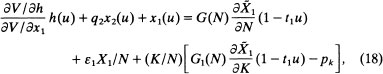
where ε₁ is defined as (dG₁/dN)(N₁/G), the elasticity of scale effects with respect to city population; and X₁ is the total net city output of X₁.

The left-hand side of equation (18) is the social cost to the economy of adding one resident to the city. This is the value of a new resident’s consumption of x₁, x₂ and h (taken from the total available to the city), such that all residents have equal utility. Note that commuting times borne by this resident are not a direct social cost to the city, although any differential leisure loss borne by the new resident relative to other residents must be compensated with market goods to maintain equal utilities.

The right-hand side of equation (18) is the social benefit of an additional resident. The first term is the private marginal product of the resident and the second is his positive externality effect on total city output. Therefore, the first two terms are his social marginal product (SMP). The third term is the net benefit/loss to the city from employing the resulting additional capital to maintain the national K/N ratio in the city.

In summary, given identical residents equation (18) states that at optimal city size the marginal social benefits of increasing city size just equal the marginal social costs. This size divided into the economy’s population yields the optimal number of cities. To determine if equation (18) will be satisfied in a market economy, it must first be interpreted in a market context.

Application to a market economy. The Pareto-efficient solution relevant in a free market economy is one in which factors are paid the value of their private marginal product. In that case the capital effect—the last term of equation (18)—equals zero. The wage rate equals , the price of housing. We assume that land rental income in the city is divided equally between residents by a city land bank company or by the city government. (This avoids introducing a third class of people, or rentiers.) The left-hand side of equation (18) will be a resident’s expenditures, which must equal his income, or the wage rate plus his land rent share. Accordingly, equation (18) reduces to

This defines a general relationship that must hold in a market economy when any individual city is of efficient size. It has a simple intuitive explanation.

The benefit of an additional resident to other city residents is the increase in production available to them, ε₁ X₁/N their cost is the additional land rent share that must be allocated to the new resident. Since per-person land rent in a city starts at a miniscule level and then rises with city size and marginal scale effects are positive (but perhaps declining), the net benefit of additional residents starts off positive and then declines to zero at optimal city size, as land rent shares increase and scale effects wane.

Will the market generate Pareto efficient solutions? Under the assumption of only one type of city, equations (18) and (19) are generally satisfied in stable market solutions. Henderson (1977, Chs. 3, 4) as well as Stiglitz (1977), Arnott (1979), Arnott and Stiglitz (1979), Kanemoto (1980), and Hochman (1981) have demonstrated this in a general equilibrium model of a system of monocentric cities, where satisfying this condition is necessary for stable market solutions. For example, if cities are larger than those specified by equation (18) a developer could set up a city of efficient size, pay competitive capital rentals and utility levels, and have a profit left over (this must be, since the monetized sum of possible utility levels plus capital rentals is higher at the efficient city size than otherwise). Other entrepreneurs would adjust their existing or potential city sizes in an effort to duplicate these profits and this adjustment process will move market solutions to efficient ones.

The Pareto-efficiency of market solutions in this context also makes sense from an externality perspective. Laborers move to equalize private marginal location benefits between cities, whereas, from a social perspective, they should incorporate into their calculus any external effects of migration and equalize social marginal location benefits. However, because in this simple situation all cities are identical, the magnitude of external effects will be equal between cities; and when laborers move to equalize private location benefits they will also incidentally equalize social benefits.

All this discussion assumes there are many cities in the economy, so that when the city size implicit in equation (19) is divided into the national population to get the equilibrium integer number of cities, any remainder can be divided amongst the equilibrium number of cities with an infinitesimal impact on individual sizes. If this large economy assumption is inappropriate, the analysis is more complicated (Henderson, 1974) and equation (19) is incorrect. This problem is discussed more extensively in Section 2.2. However, the problem has not been truly dealt with in the literature. For example, it is no longer clear that it is always optimal to treat cities of the same type identically, a constraint we imposed. A solution with many cities satisfying (19) but not all could dominate a solution where all cities are identical.

Public goods. So far, it has been assumed that external economies of scale are the basis for agglomeration in cities. Suppose instead or in addition that people agglomerate in monocentric cities to exploit the Samuelson publicness of public goods. In the optimization problem outlined at the beginning of this section, pure public goods would enter utility functions and public service costs would enter the balance-of-trade constraint. Optimizing yields the same optimal population condition as does equation (18), given that an additional resident may consume the existing level of pure public goods at zero cost. The market interpretation of equation (18) is the same, except that residents are taxed to finance public services. If we assume that public services are provided on an equal cost-share for equal-income residents and that marginal (but not necessarily intramarginal) scale effects, or ε₁ are zero, the market interpretation of equation (19) becomes (Henderson (1977b))

To city residents, the marginal cost of an additional resident is the land rent share that he gets and the marginal benefit is the tax share he incurs.

This result was originally derived by Flatters, Henderson, and Mieszkowski (1974) in a regional Ricardian increasing cost model, in which a system of regions is generated much like a system of cities, and has been extensively developed by Arnott (1979) and Arnott and Stiglitz (1979)). Another implication of equation (20) is that total taxes equal total public expenditures, which equal total land rents in a city. Public services may be financed best by taxing away all land rental income and using only that revenue to finance public services. (This implication does not depend on the way in which land rent income is distributed (Flatters, Henderson, and Mieszkowski, 1974).) This is equivalent in a local context to Henry George’s 1879 proposal that public expenditures be financed solely by a tax that taxes away all land rental income (above frontier rents, which are zero agricultural rents here) (George, 1938). This analysis is thus a modern vindication of George’s proposal.

Multiple types of cities. So far, we have discussed city size when there is only one type of city. Suppose that there are two or more types of city. To illustrate the basic problem of having non-identical types of cities, we start by assuming there are only two types of city, one specializing in X₁ production and the other in X₂ production and that there is adequate economy population for just one city of each type, so that the optimization problem is simply to allocate the population between the two cities. Thus cities will probably not be of individually efficient size and the optimal number of cities is assumed at the outset to be two.

The optimization problem outlined above can easily incorporate a second type of city by the addition of employment, spatial, and equal utility constraints for the second type of city and by the use of full-employment and production-consumption constraints for the economy as a whole. Given the new optimization problem, the optimal population allocation condition becomes (Henderson, 1977b, Chap. 4)

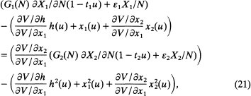
where ε₁ and ε₂ are scale effect elasticities. In the first [second] line of equation (19), following the discussion of Section 1, the first expression in large parentheses is the social marginal product (SMP) of labor in city X₁. The second expression is the consumption cost, or social marginal cost (SMC), of labor in city X₁. Therefore, equation (21) may be written informally as

This states that the gap between SMP and SMC should be equalized in all cities. For example, if SMP₁, – SMC₁ > SMP₂ – SMC₂, city X₁ is underpopulated. Since the gap between per-person productivity and consumption is greater in city X₁, a person may be moved from city X₁ to city X₂ without affecting utility levels and there would be a residual of goods leftover.

The basic concern is whether equation (21a) will be satisfied in a market economy. The problem in attaining efficient city sizes, given more than one type of city, is due to the existence of different degrees of external scale economies in different types of city. If marginal scale economies differ between cities, laborers will not equalize social location benefits when they move to equalize private location benefits between cities. To determine under what conditions a city may be over- or underpopulated in a market economy, we interpret equation (21a) in a market context in which land rents are distributed equally among residents of a city. Following the derivation of equation (19), equation (21) becomes

Suppose the X₁ city is larger than the X₂ city (due to differences in intra-marginal scale economies or relative export demands), so that land rent shares are probably greater in X₁ cities. If marginal scale effects are lower [higher] in X₁ cities, then X₁ cities must be overpopulated [may be underpopulated]. In either case, to encourage optimal population movement, federal intervention will be necessary to tax people in overpopulated cities or subsidize people in underpopulated cities.

Note that this analysis rejects a partial equilibrium approach to the determination of optimal city size. Under an approach in which each city is viewed on its own, if SMP > SMC for a city, immigration should be subsidized. This is incorrect since such a policy would draw population from other cities where SMP > SMC. Immigration should only be subsidized if the gap between SMP and SMC is greater in some cities than in others.

This externality analysis is concerned with population allocation at the margin. In the present context there is another problem. Cities are individually best off by satisfying equations (18) and (19), where SMP = SMC; whereas with a limited number of cities, Pareto-efficient solutions for the economy as a whole usually involve a gap between SMP and SMC. This provides a basis for individual cities to non-optimally try to restrict (or enhance) their size and force some of the population into additional very small, inefficient size cities.

If there are many cities of each type, however, both this global problem and the externality population allocation problem disappear, as explained above. As the number of cities of each type increases, the gap between SMP and SMC in each type of city declines until at the limit it is zero; or all cities can approach their individually efficient size (the remainder problem referred to above disappears). Then equations (18), (19), (21), and (22) will all be satisfied. Thus the basis for non-optimality is the problem remainders mentioned initially. In a “large” economy, the remainder problem becomes negligible and markets generate efficient city sizes, despite the presence of externalities.

Pure public goods. If we reintroduce pure public goods as the basis for urban agglomeration, in an economy with a population adequate for only one X₁ and one X₂ type city, the optimal population allocation condition is the same as equation (19). Interpreting this in a market context, assuming public services are financed by equal tax shares for similar people and assuming marginal scale economies, ε, are zero, yields:

To add a twist and to isolate the public good problem, assume that land rents go out of the system to a separate group (rentiers). Then (23) becomes

When will this condition be satisfied in a market economy? Suppose that X₁ cities are larger (due, say, to greater intra-marginal scale economies). The unit tax price of public goods is 1/N, where N is city population and the unit cost of public services is set at 1 unit of X₁, Since N is larger in the city X₁ the per-person unit tax price is lower. The relative levels of per-person public expenditures and tax shares between cities is determined by the compensated price elasticity of demand for public services. If this elasticity equals |–1|, per-person expenditures and taxes will always be equal between cities, regardless of tax prices, given equal utility levels between cities. However, if the elasticity is greater [less] than |–1|, expenditures are greater in the low [high] tax price X₁ [X₂] city; and the X₁[X₂] city is underpopulated. Thus optimality generally requires federal intervention.

This problem in public service provision has been termed a fiscal externality, in the sense that when a person migrates he affects the tax prices of all residents in the cities he enters or leaves, but he does not account for these effects in making his migration decisions. It is also useful to view the problem from another perspective. From equation (23a), this problem of potential misallocation of population can be solved by the allocation of tax shares on a national basis (so that similar people pay the same taxes regardless of location)—the same comments apply to the distribution of land rent shares when evaluating equation (23). Tax shares do not in themselves affect or directly represent production or consumption capabilities in the economy; therefore, we want to ensure that they do not influence location decisions. Equalizing shares nationally will remove any incentive to move based on tax shares; location decisions will be based solely on local marginal productivity and public good consumption conditions. However, with national financing, the national government would have to pay for local public services, which presents the problem of the correct assessment of local preferences and the satisfaction of the local Samuelson condition in the provision of local services.

As analyzed in Flatters, Henderson, and Mieszkowski (1974), the introduction of other externalities (such as congestion in public good consumption or transportation, pollution and so on) simply adds additional terms to each side of equations (21) and (23) that state the magnitude of the particular externality. To evaluate the over- or underpopulation of a city or region one simply adds the different externality effects for a city and compares the totals for different cities. Empirically, some initial attempts at this type of exercise have been made (Tolley, et al. (1979)). They generally indicate that there may be large overpopulations of some metropolitan areas, but that the welfare losses of these overpopulations are very small.

References

Arnott, R. (1979), “Optimum City Size in a Spatial Economy”, Journal of Urban Economics, 6, 65–89.

Arnott, R. and J. Stiglitz (1979), “Aggregate Land Rents, Expenditure on Public Goods, and Optimal City Size”, Quarterly Journal of Economics, 471–500.

Baer, W. (1969), The Development of the Brazilian Steel Industry, Vanderbilt University Press.

Beckmann, M. J. (1958), “City Hierarchies and Distribution of City Size”, Economic Development and Cultural Change, VI, 243–48.

Beckmann, M. J. (1968), Location Theory, Random House, New York.

Berglas, E. (1976), “The Distribution of Tastes and Skills and the Provision of Local Public Goods”, Journal of Public Economics, 6, 409–423.

Bergsman, J., P. Greenston, and R. Healy (1972), “The Agglomeration Process in Urban Growth”, Urban Studies.

Bergsman, J., P. Greenston, and R. Healy (1975), “A Classification of Economic Activities Based on Location Patterns”, Journal of Urban Economics, 2, 1–28.

Carlino, G. A. (1978), Economics of Scale in Manufacturing Location: Theory and Measurement (Leiden: Martinus Nijhoff).

Chipman, J. S. (1970), “External Diseconomies of Scale and Competitive Equilibrium”, Quarterly Journal of Economics, 84, 347–85.

Christaller, W. (1966), The Central Places of Southern Germany, Englewood Cliffs: Prentice-Hall.

Dixit, A. (1973), “The Optimum Factory Town”, Bell Journal of Economics and Management Science, 4, 637–654.

Flatters, F., V. Henderson, and P. Mieszkowski (1974), “Public Goods, Efficiency, and Regional Fiscal Equalization”, Journal of Public Economics, 3, 99–112.

Fogel, R. (1964), Railroads and American Economic Growth, Baltimore: Johns Hopkins Press.

Getz, M. and Y. Huang (1978), “Consumer Revealed Preference for Environmental Goods”, Review of Economics and Statistics, 449–458.

Haurin, D. (1980), “Population Migration and Climate”, Quarterly Journal of Economics, 293–308.

Henderson, J. V. (1972), “The Sizes and Types of Cities: A General Equilibrium Model”, Unpublished Ph.D. dissertation, University of Chicago.

Henderson, J. V. (1974), “The Sizes and Types of Cities”, American Economic Review, 64, 640–656.

Henderson, J. V. (1977a), “Externalities in a Spatial Context: The Case of Air Pollution”, Journal of Public Economics, 7, 89–110.

Henderson, J. V. (1977), Economic Theory and the Cities, Academic Press, New York.

Henderson, J. V. (1982a), “The Impact of Government Policies on Urban Concentration”, Journal of Urban Economics, 12, 280–303.

Henderson, J. V. (1982b), “Systems of Cities in Closed and Open Economies”, Regional Science and Urban Economics, 12, 325–350.

Henderson, J. V. (1982c), “Evaluating Consumer Amenities and Interregional Welfare Differences”, Journal of Urban Economics, 11, 32–59.

Henderson, J. V. (1985), “Population Composition of Cities: Restructuring the Tiebout Model”, Journal of Public Economics, 27, 131–156.

Henderson, J. V. (1986a), “Urbanization in a Developing Country: City Size and Population Composition”, Journal of Development Economics, 22, 264–293.

Henderson, J. V. (1986b), “Efficiency of Resources Usage and City Size”, Journal of Urban Economics, 19, 47–70.

Henderson, J. V. and Y. Ioannides (1981), “Aspects of Growth in a System of Cities”, Journal of Urban Economics, 10, 117–139.

Hoch, I. (1977), “Climates, Wages, and Quality of Life”, in Public Economics and the Quality of Life (L. Wingo and A. Evans, eds.), pp. 28–65, Johns Hopkins Press, Baltimore.

Hochman, O. (1977), “A Two Factor Three Sector Model of an Economy with Cities: A Contribution to Urban Economics and International Trade Theories”, (mimeo.).

Hochman, O. (1981), “Land Rents, Optimal Taxation, and Local Fiscal Independence in an Economy with Local Public Goods”, Journal of Public Economics, 59–85.

Izraeli, O. (1979), “Externalities and Intercity Wage and Price Differentials”, in Urban Grown Policy in a Market Economy (G. Tolley, et al., eds.), Academic Press, New York.

Jones, R. W. (1968), “Variable Returns to Scale in General Equilibrium”, International Economic review, 10, 261–272.

Kanemoto, Y. (1976), “City Sizes: Optimum vs. Market”, mimeo.

Kanemoto, Y. (1978), “Optimal Growth of Cities”, Discussion Paper 78–02, University of British Columbia, mimeo.

Kanemoto, Y. (1980), Theories of Urban Externalities, North-Holland.

Losch, A. (1954), The Economics of Location, New Haven.

Mayer, W. (1974), “Variable Returns to Scale in General Equilibrium”, International Economic Review, 15, 225–235.

Mills, E. S. (1967), “An Aggregative Model of Resource Allocation in a Metropolitan Area”, American Economic Review, 57, 197–210.

Mills, E. S. (1972), Urban Economics, Scott Foresman, 1st edition.

Mirrlees, J. A. (1972), “The Optimum Town”, Swedish Journal of Economics, 74, 114–135.

Miyao, T. (1981), Dynamic Analysis of an Urban Economy, Academic Press.

Neary, J. P. (1978), “Dynamic Stability and the Theory of Factor-Market Distortions”, American Economic Review, 68, 671–682.

Parr, J. B. (1969), “City Hierarchies and the Distribution of City Size”, Journal of Regional Science, 9, 239–254.

Rosen, S. (1979), “Wage-Based Indexes of Urban Quality of Life”, in Current Issues in Urban Economics (P. Mieszkowski and M. Straszheim, eds.), Johns Hopkins Press, Baltimore.

Segal, D. (1976), “Are There Returns of Scale in City Size”, Review of Economics and Statistics, LVIII, 339–50.

Shefer, D. (1973), “Localization Economies in SMSA’s: A Production Function Approach”, Journal of Regional Science, 13, 55–64.

Starrett, D. A. (1974), “Principles of Location in a Large Homogeneous Area”, Journal of Economic Theory, IX, 418–48.

Stiglitz, J. E. (1977), “The Theory of Local Public Goods”, in The Economics of Public Services, M. S. Feldstein and R. P. Inman (eds.), Macmillan.

Sveikauskas, L. (1975), “The Productivity of Cities”, Quarterly Journal of Economics, 89 393–413.

Sveikauskas, L. (1978), “The Productivity of Cities”, mimeo., 1–94.

Thomas, V. (1978), “The Measurement of Spatial Differences in Poverty: The Case of Peru”, World Bank Staff Working Paper #273.

Tolley, G. et al. (1979), Urban Growth Policy in a Market Economy, Academic Press.

Upton, C. (1981), “An Equilibrium Model of City Sizes”, Journal of Urban Economics, 10, 15–36.

Vickrey, W. (1977), “The City as a Firm” in The Economics of Public Services, M. S. Feldstein and R. P. Inman (eds.), Macmillan.

Wheaton, W. (1974), “A Comparative Static Analysis of Urban Spatial Structure”, Journal of Economic Theory, 9, 223–237.

Yezar, A. and R. Goldfarb (1982), “An Indirect Test of Efficient City Size”, Journal of Urban Economics, 5, 46–65.

¹ An explanation of the problem in the traditional stability of trade framework is straightforward. Start with a situation where the relative domestic price of X₂, equals the world price and shock the system so X₂/X₁ increases. In a traditional framework it is assumed all factor markets instantaneously adjust to maintain equilibrium (at new U and r’s) in factor markets, so if X₂/X₁ changes, must change. Stability requires that if X₂/X₁ increases rises (above so producers of X₂ take a loss, X₂ production is reduced, and hence we move back towards the original equilibrium. If instead when X₂/X₁ increases falls, then producers of X₂ experience profits, in response X₂ production is further increased and we flee from the original equilibrium. In our model if X₂/X₁ increases, rises if k₂ > k₁ when α₂ < α₁. The intuitive explanation is as follows. As X₂/X₁ rises, will only rise if the relative price of the factor X₂ uses intensively rises. r/w and hence q₂ will only rise if k₂ falls (and hence k₀₂ = K₀/N₀ in X₂ production falls). If k₂ > k₁ as X₂/X₁, increases by shifting production from type 1 to type 2 cities, k₂ and k₁ must necessarily fall to maintain full employment (in standard trade models this is illustrated in an Edgeworth box diagram). Hence, d/d(X₂/X₁) > 0 if k₂ > k₁. However, if k₁ > k₂, as X₂/X₁ rises k₂ and k₁ must rise; hence r/w will fall, hence will fall.

There are some more general stability frameworks (Mayer, 1974 and Neary, 1978). Neary (1978) has criticized this classical adjustment process as being bizarre, because it assumes factor markets adjust completely to each potential price (), even though the final price is a parameter. Neary examines local stability in an entirely different adjustment model where capital and labor do not move instantaneously among sectors and must always equal in an open-market economy. Then the impact of a shock is to create disequilibrium in factor markets, in terms of the allocation of factors between sectors. Henderson (1982b) adapts this framework in analyzing the allocation of factors between types of cities and shows stability of a nonspecialization equilibrium still requires k₂ > k₁ when α₂ > α₁ Hochman (1977) notes that this problem threatens the stability of closed economy equilibrium given Hicksian static “stability” conditions are not met.