
2
FUNDAMENTALS OF DATA STRUCTURES — BASIC CONCEPTS
Computer science is primarily concerned with the study of data structures and their transformation by some techniques. The modern digital computer was invented and intended as a system that should facilitate and speed-up complicated and time-consuming computations. In the majority of applications its capability to store and retrieve large amount of information plays a dominant role in processing information. The information which is available to the computer consists of selected set of data relating to a real-world problem and it is believed that the desired results can be derived from those set of data. So it is desirable to understand the logical relationships between the data items in the problem. The possible ways in which the data items or atoms are logically related define data structures.
2.1 INTRODUCTION TO DATA STRUCTURE
A data structure is a data type whose values are composed of component elements that are related by some structure. Since a data structure is a data type, it has a set of operations on its values. In addition, there may be operations that act on its component elements. A number of operations can be performed on a data structure, operations for inserting elements into and deleting elements from a data structure, and operations to access an element from a data structure. These operations vary functionally for different data structures. The operations associated with a given data structure depend on how the data structure is represented in memory and how they are being manipulated by a particular language. The representation of a particular data structure in the memory of a computer is called a storage structure. For example, there are a number of possible storage structures for a data structure of an array. It is thus clear that data structures, their associated storage structures, and the operations on data structure are all integrally related to the particular problem. In this book we will examine different types of data structure and their implementation through C language.
A number of applications, using various kind of data structure, will be discussed in a comprehensive manner throughout the book. The choice of an algorithm description notation must be crucial since they play a vital role in implementing applications. In the next section, algorithm, a fundamental notion, will be discussed.
2.2 ALGORITHM FOR DATA STRUCTURE
An algorithm represents an abstract level the steps that a computer takes to do a job. We required that only the steps of an algorithm be well-understood, and stipulated that the expression of an algorithm may vary with the level of understanding of its audience.
An algorithm is a formal step-by-step method for solving problems. An algorithm should satisfy the following properties.
• An algorithm consists of a sequence of instructions.
• Each instruction should be unambiguous.
• Each instruction should comprise a finite set of instructions.
• The algorithm should terminate after a finite number of steps.
• The algorithm may have an input but it should produce an output.
It is now necessary to introduce the concept of the mathematical tools needed to analyze the algorithms and data structures that will be discussed in the rest of the chapters. The analysis of algorithms is a critically important issue in computer science. The data structures that we would discuss (e.g. array, stacks, queues, link lists etc.) are not only mathematically interesting but we also claim that they play a vital role in developing efficient algorithms for such tasks as insertion, deletion, searching, sorting, and pattern matching. How do we show that this claim is valid? We should demonstrate the algorithms for a given application without depending on informal arguments, without considering special cases, and without being influenced by the efficiency of the programming language used to encode the algorithm or the hardware used to run it. We introduce a technique which is the fundamental tool for evaluating the efficiency properties of algorithms. The notion introduced here is used throughout the study of data structures and algorithms. The notion includes complexity measures, order notation, detail timing analysis, and space complexity analysis.
The mathematical notation used in this book has been selected from notation commonly used in data structures. This notation tends to differ only slightly from that in general use in the mathematical literature. For example, log x may be written as lg x in some places. Other notations are defined at the point of first use with explanation. Algorithm notations, if any used, will be discussed at the time of presentation.
In describing algorithms, we emphasize upon certain points. First, algorithms should be concise and compact to facilitate verification of their correctness. Verification involves observing the performance of the algorithm with a carefully selected set of test cases. These test cases should attempt to cover all the exceptional cases likely to be encountered by the algorithm. Second, an algorithm should be efficient. They should not unnecessarily use memory locations nor should they require an excessive number of logical operations.
In the next section, we give a description of the algorithm notation.
2.3 NOTATION FOR ALGORITHM
Once we have an appropriate mathematical model for a problem, we can formulate an algorithm in terms of that model. The notation used to present algorithms is widely used with minor variation in the literature on data structures. Normally, we follow the order (as given below) throughout the book for describing a method.
(i) Basic concept of the method.
(ii) Illustration of the method with suitable data.
(iii) Algorithm for the method.
(iv) C program for the method.
Let us write a simple algorithm for finding maximum from a set of n positive numbers. We assume that numbers are stored in an array X. We hope that these instructions are sufficiently clear so that the reader grasps our intention.
Algorithm 2.1: Searching a maximum from an array X
Input: An array, X, with n elements.
Output: Finding the largest element, MAX, from the array X.
Step 1: Set MAX=0/* Initial value of MAX*/
Step 2: For j= l to n do
Step 3: If (X[j]>MAX) then MAX=X[j]
end for
Step 4: Stop
Each algorithm in this book is given a number and a title. The title immediately follows the algorithm number on the same line. Inputs and outputs are described next. The body of the algorithm consists of a set of numbered steps (the word ‘step’ before the number). Comments (similar to C comments) may appear in steps of an algorithm to help the reader in understanding the details. For example, the remark /* initial value of MAX */ appears at Step 1. Different constructs such as for-do-end, if-then, while-do, and so on are used very similar to pseudolanguage. It is important to emphasize that data structures are language independent. Pseudocode is a general tool that allows notation similar to any high-level language.
An algorithm can be described in many ways. As described earlier, pseudocode can also be used to represent an algorithm. Another way we can express an algorithm is through a graphical form of notation such as flowcharts. In case of complex decisions, it is difficult to understand the decisions either in flowcharts or through pseudocode. Decision table is an alternative analysis tool for indicating complex relationships and solutions. In view of this, we start our discussion through the basic concepts of flowcharting for expressing an algorithm.
2.3.1 Flowcharts
A flowchart is a pictorial representation of an algorithm. It serves as a means of recording, analyzing, and communicating problem information. Programmers often use a flowchart before writing a program. It is not always mandatory to draw a flowchart. In practice, sometimes, drawing of the flowchart and writing of code in a high-level language go side by side.
Two kinds of flowcharts are used—program flowchart and system flowchart. A program flowchart (also called a flowchart) shows the detailed processing steps within one computer program and the sequence in which those steps must be executed. Different symbols are used in a flowchart to denote the different operations that take-place in a program. Terminal symbol ![]() shows clearly the beginning and ending of the program. The symbol
shows clearly the beginning and ending of the program. The symbol ![]() denotes the input/ output operation. Any manipulating or processing of data within the computer is expressed by the processing symbol
denotes the input/ output operation. Any manipulating or processing of data within the computer is expressed by the processing symbol ![]() In a flowchart the decision symbol
In a flowchart the decision symbol ![]() is used to specify a conditional branch or decision-making step. Connector symbols
is used to specify a conditional branch or decision-making step. Connector symbols ![]() are used in a flowchart to denote exit to or entry from another part of the flowchart.
are used in a flowchart to denote exit to or entry from another part of the flowchart.
A system flowchart shows the procedures involved in converting data on input media to data in output form. Emphasis is placed on the data-flow into or out of a computer program, the forms of input and the forms of output. A system flowchart makes no attempt to depict the function-oriented processsing steps within a program. A system flowchart may be constructed by the systems analyst as part of the problem definition. However, algorithms in data structure are always expressed in the form of flowcharts.
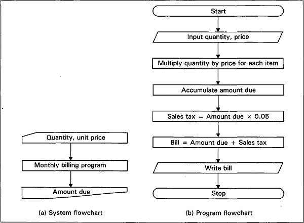
Fig. 2.1 System and program flowcharts for monthly billing
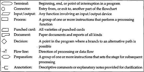
Fig. 2.2 System and program flowchart symbols
A system flowchart for monthly billing is show in Fig. 2.1(a) to emphasize a distinction between a system flowchart and a flowchart, a flowchart showing the detailed processing steps in the monthly billing program is given in Fig. 2.1(b).
In drawing flowcharts we call directly our attention to the standard flowcharting symbols and techniques recommended by the American National Standards Institute (ANSI) and its international counterpart, the International Organization for standardization (ISO). These symbols are used throughout the book. These symbols are summarized in Fig. 2.2.
The program flowchart in Fig. 2.1 has one serious drawback; it shows how to compute the monthly statement for only one customer. Generally, a computer program is written to perform a particular operation or sequence of operations many times. To provide for this, a program flowchart can be made to curve back on itself, that is, a sequence of processing steps can be executed repeatedly on a different set of data. In effect, a program loop is formed. We now present the modified flowcharts in Fig. 2.3.
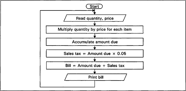
Fig. 2.3 Program loop through unconditional jump
2.3.2 Pseudocode
Pseudocode is referred to as a pseudolanguage or an informal design language. Its primary function is to enable the programr to express his/her ideas about program logic in a very natural english-like form. He/she is free to concentrate on the solution algorithm rather than on the form and constraints within which it must be stated. The intended result is an unambiguous solution to the problems.
Pseudocode allows a programr to express his/her thoughts in regular english phrases, with each phrase representing a programming process that must be accomplished in a specific program module. The phrases almost appear to be programming language statements, thus the name ‘pseudocode'. However, unlike programming language statements, a pseudocode has no rigid rules; only a few optional keywords for major processing functions are recommended. Therefore, programmers can express their thoughts in an easy, natural, straightforward manner, but at a level of detail which allows pseudocode to be directly convertible into programming-language code. Fig. 2.4 provides pseudocode for salesperson payroll program.
   begin
      Read a salesperson payroll record
      do while there is more data
          multiply sales by commission rate
          if sales is greater than quota
                 then add 10% bonus to commission
          endif
          add commission to salary
          write a report line
          read a salesperson payroll record
      enddo
   end
Fig. 2.4 Pseudocode for salesperson payroll report processing
Certain words in a pseudocode are significant. ‘Input’ or ‘read’ a record means that data is made available to the computer for processing. The input data is generally in the form of a record, for which several fields of data pertaining to a person or thing are given as one-line input or one item. If the data pertained to employee records, a record might contain the employee identification number, the department to which that employee is assigned, the number of hours worked, the rate per hour, and the tax deduction.
The word ‘set’ or ‘assign’ is often used in a pseudocode to initialize values to a desired amount. The word ‘if’ in the pseudocode indicates comparison between two items. Sometimes the words add, subtract, multiply, or divide appear in a pseudocode but this often is the choice of the programmer. Another word used in the pseudocode is ‘print’ or ‘write’. It indicates that data is to be prepared as output on the printer. Other words, such as do-enddo, dowhile-endwhile, are used. We will now illustrate examples of pseudocode.
Example 2.1
      begin
            do
                  read a record of three numbers
                  print elements in record
                  compute sum of elements
                  print sum
            enddo
      end
Example 2.2
      begin
            read a record-hours worked, rate, tax
            multiply rate by hours worked and set it to gross pay
            compute netpay = gross pay - tax
            write hours worked, rate, tax, gross pay, net pay
      end
We now present another pseudocode for insertion sort with a procedure insertion sort. It takes as a parameter an array A[l]-A[n] containing a sequence of length n which is to be sorted. Insertion sort works the way many people sort cards. We start with an empty left hand and cards face down on the table. We then remove one card at a time from the table and insert it into the correct position in the left hand. To find the correct position for a card, we compare it with each of the cards already in the hand from right to left.
    /* Pseudocode for insertion sort */
    Insertion Sort(A)
    begin
        for J←2 to length (A) /* length (A) means length of A */
              key←A[J]
    /*  Insert A[J] into the sorted sequence A[1]…A[J—1] */
        i←J—1
        while i > 0 and A[i]> key
                 A[i+1]←A[i]
                 i←i-1
        endwhile
        A[i+1]←key
        endfor
    end
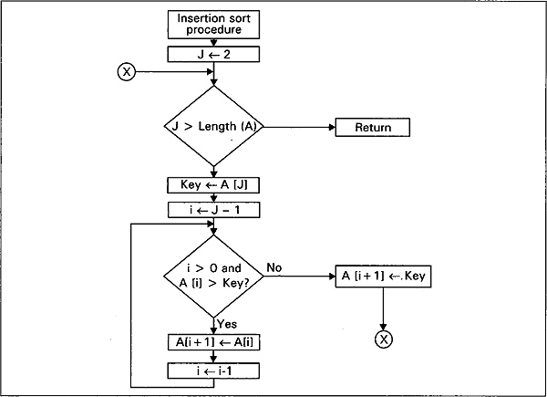
Fig. 2.5 Flowchart for insertion-sort procedure
The above insertion sort procedure can be graphically described by the flowchart shown in Fig. 2.5.
2.3.3 Decision Tables
Tables are a familiar, widely used mode of representing and communicating information. When we buy groceries and other items at the local shop, the shopowner/cashier at the counter refers to a table that shows a list of items and the price for each. Airlines use tables that show destinations and distances, or destinations and fares. There are applications too where table plays a vital role. What is the advantage of using such tables? They are easy-to-follow means of communication. They are also a concise way of representing information. They represent a way of giving a number of complex decisions in a tabular form; for much the same reasons, tables can be an effective tool in program development. Sometimes a team programr assigned to a particular part of a project may set up one or more tables when planning a solution to an algorithm. Each table serves as a guide during program coding. A table used in this way is known as a decision table. The purpose of this section is to explain how to use decision tables and how to construct them. We look at different types of decision tables that can be built and the situations for which they are useful.
A decision table is used for defining complex program logic. It is preferred by some programrs because decision tables can be constructed quickly. One advantage of using a decision table is that it is easier to construct than a flowchart since no symbols are involved. Phrases are not as difficult to use in a decision table, which is not as limited in space as a flowchart.
A decision table would simply show the possible numbers of dependents as a series of conditions. The processing steps needed to compute the appropriate deductions would be listed as actions. As shown in Fig. 2.6, a decision table is divided into four sections. The upper left portion is called the condition stub. It shows the conditions that are to be considered in reaching a decision. The lower left portion is called the action stub and it shows the actions to be taken when any of the given sets of conditions is present. The condition entries in the upper-right portion of the decision table and the action entries in the lower-right portion illustrate clearly each if-then-else to be followed. To understand a rule, we read vertically the columns that are a set of condition entry and action entry forms. The number of the rule appears at the top of the column. More than one action may be required if the applicable conditions may exist. In other words, both multiple condition entries and multiple action entries for a particular rule are possible in some cases.
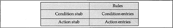
Fig. 2.6 Decision table format
Let us consider some examples to illustrate the use of a decision table.
Example: If an employee's attendance sheet indicates that he or she worked less than ten hours during the past week, or that he or she was late more than once, or that he or she was absent on the day before a holiday, then the employee's name should be deleted from the payroll list, otherwise that employee's payroll cheque should be printed.
In the above example, three conditions are identified but any one of the three conditions will produce a certain action. If an employee worked less than 10 hours, his or her name should be deleted from the payroll list, irrespective of whether or not he or she was late more than once or absent on the day before a holiday, and so on. The decision table is shown in Fig. 2.7. For each of the three possible conditions, the condition entry in a column may be Y for ‘yes’ or N for ‘no'. The action entry contains an ‘X’ for the satisfying conditions.
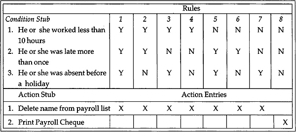
Fig. 2.7 Decision table for example
Another very useful and alternative representation of a decision table is decision tree. We now present decision tree and the corresponding flowchart for the six-coin problem in Figs. 2.8 and Fig. 2.9. Given coins a, b, c, d, e, and f, we want to find out the heavier coin with the property that one is heavier but rest are equal.
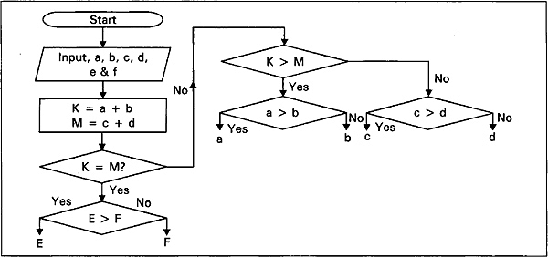
Fig. 2.8 Flowchart for the heavier coin among coins a, b, c, d, e and f
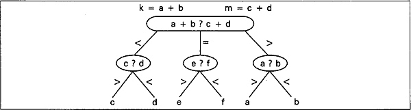
Fig. 2.9 Decision tree for finding the heavier coin among coins a, b, c, d, e and f
2.4 MODULARISATION TO ALGORITHM DESIGN
The medium and large sized software projects in real world might be decomposed into as many as one hundred to one thousand separate pieces. The step in the programming process involves taking the problem described in the problem specification document and decomposing it into a collection of interrelated subproblems, each of which is much smaller and much simpler than our original task. This decomposition of the problem is an example of the design technique called divide and conquer, which is based on the principle that it is easier to solve many small problems than to solve one extremely large one.
Modularisation is the formal term for the divide and conquer strategy. (It allows us to compartmentalise a large problem into collections of independent program units that address simpler and more coherent subproblems.) Each independent program unit is called a module. Modules are the functional parts that make the processing work. Ideally, each module works independently of the other modules, although this sometimes is impossible. Relate the concept of using modules or steps that could be listed—purchasing of the necessary ingredients, the preparation of the ingredients, and the baking of the cake. Under each of the three modules, the details would be listed. Modules are ranked by hierarchy as to importance. The lower the module on the structural organisation plan, the more detail is given as to the programming steps involved. The top module works as a control module, which gives the overall view of the structure for the program. The program is designed so that at each level of module, more detail is given.
Each module is coded and tested and is then added to the other modules. This procedure makes program integration easier since there is a single entry and one exit point per module. This makes any further modification of a program easy since we know that there is only one way to enter the module and one way to exit.
Modularisation brings with it a number of distinct benefits. First, it greatly simplifies the task of modifying or adapting a program unit. Since the only part of a module visible to the rest of the modules is its external interface, a change to the internal structure of a module should have no effect on any other module. Modularisation allows us to hide the underlying implementation details of one program unit from all other program units and protect it from unauthorised change.
Second, modularisation helps us with a way to create an implementation plan. If we can create a chart that shows the relationships among these units, we have the means to create such an implementation plan.
Another advantage of modularisation is that we can verify each individual program unit for corrections as it is developed, instead of having to wait until the entire program is completely coded. As program units get larger, debugging time increases drastically, eventually becoming the dominant step in the entire programming project. It is definitely to our advantage to debug and test a program as a collection of small units rather than one large one.
The important point is that having modularised the problem and developed it in a top-down fashion, we have a choice of ways to approach the implementation. As we work on one unit, we know what unit we should work on next and which ones can be effectively postponed. Without this plan of action, we might write code in some less logical order and thus not have pieces that work together or that can be tested as a unit. The top-down design method, which develops as a hierarchical set of tasks, defines a natural set of small sub-units that can be individually tested, verified, and integrated into the overall solution. In the next subsection we describe the top-down design method.
2.4.1 Top-down Design Approach
Top-down design involves starting from the broadest and most general description of what needs to be done, that is, the problem specification document, and then sub-dividing the original problem into collections of modules and abstract data types. Each of these lower-level units is smaller and simpler than the original task and is more involved with the details of how to solve the problem rather than what needs to be done. We proceed from high-level goals to detailed low-level solution mothods.
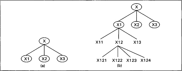
Fig. 2.10 Pictorial representation of top-down approach
We consider a program X that can be subdivided into three independent submodules, X1, X2, and X3. These submodules, Xl X2, and X3 are further broken down into independent submodules, and so on. This process is repeated until we obtain modules which are small enough to be understood and coded quite easily. We can represent it pictorially as shown in Fig. 2.10.
Top-down design is not the one-step process as shown in Fig. 2.10(a). The decomposition and simplified task is performed over and over. First on the original problem and then on successive sub-units until finally we are left with a task that is so elementary that it need not be simplified any further. The repeated decomposition and simplification of a task into a collection of simpler sub-tasks is called stepwise refinement. Each of the tasks X in Fig. 2.10(b) represents a separate program until needed to solve the original problem.
The data structures needed for the solution are also developed in a top-down fashion as we proceed from general descriptions of abstract data types to operations performed on these data types to their internal implementation. Next we will decide on the internal structure for our abstract data types and write the internal module that implements the operations. When we have finished refining our program units and abstract data types, we would have created a large number of procedures and data structures, defined in terms of the information they contain and the operation that can be performed on them. Description of these modules and data structure constitute a major component of the program design document.
Abstraction refers to dealing with an operation from a high-level viewpoint, disregarding its detailed structure. This will help to hide the design details of the lower-level modules to the higher-level ones. Only the data and control are specified for communication between the higher-and lower-level modules.
Procedural abstraction and data abstraction are the fundamental tools for managing the implementation of large programs, both are used in the top-down design method. With procedural abstraction we initially think only about the highest-level functions and procedures needed to solve the problem. The specification of low-level routines is postponed until later. Each successive refinement of the design adds additional detail to the developing solution. So the complexity level increases as we proceed through the design process.
With data abstraction, we initially view a data structure in terms of the external interface it displays to the user, that is, the operations that can be performed on that structure. Only later do we begin to concern ourselves with the underlying details of the implementation of that data type in a given programming language.
Modem program design techniques focus on stepwise refinement. Stepwise refinement produces software design in a top-down manner. Stepwise refinement is an iterative process. At each step, the problem to be solved is decomposed into subproblems that are solved separately. Thus, if P is the statement of the original problem, p1, p2,…, pn are the statements of the sub-problems to be solved iteratively. The following is a description of the sort-by-straight selection algorithm by stepwise refinement.
Example 2.3
 Step 1
      Let n be the length of the array A to be sorted
            i=l
            while i<n do
                  Place the smallest element at position i
                  i=i+1
            endwhile
 Step 2
      Let n be the length of the array A to be sorted
            i=1
            while i<n do
                  j =n
                        while j>i do
                              if (A[i]>A[j])
                                    interchange the elements at
                                    positions j and i
                              endif
                        j=j—1
                        endwhile
                  i=i+l
            endwhile
 Step 3
      Let n be the length of the array to be sorted
      i=l
      while i<n do
            j=n
                  while j>i do
                        if (A[i]>A[j])
                              x=A[i],A[i)=A[j],A[j]=x
                        endif
                        j=j-1
                  endwhile
                  i=i+1
      endwhile
2.4.2 Bottom-up Approach
In developing high-level application-oriented software, we will almost certainly need to make frequent references to simple, low-level procedures that do everyday housekeeping tasks. Therefore, implementation may not only be top-down but bottom-up as well. The bottom-up design moves in opposite direction of that in the top-down design method. In this design, the programmer identifies a set of essential and crucial low-level routines that would be important to be available as early as possible. Next, the higher-level modules are built upon the lower-level modules already designed. If each low-level module is coded as soon as it is designed, it is called bottom-up programming. In this technique, low-level procedures called utility routine would be implemented in parallel with or even preceeding the development of the high-level application unit. When tested and complete, these utilities are put into a program development library and are available as off-the-shelf programming tools to all the professional staff for the direction of implementation. When the most critical low-level primitives are finished, the designer may identify additional utility routines that would be desirable to have in the library. Then implementation usually proceeds in both directions, top-down for the development of high-level application oriented routines, and bottom-up for the development of utilities and programming tools to support application development.
In top-down design it is not possible to detect incompatible or unrealisable specification at an early stage since we postpone all details to the lower stages. This is a serious disadvantage to the top-down design but can be detected in bottom-up design during the early stages of the design process. On the other hand, the designer cannot find an exact idea about the entire system until the top level is reached.
According to a bottom-up strategy, the design process consists of defining modules that can be iteratively combined together to form sub-systems. This is typical in the case where we are reusing modules from a library to build a new system, instead of building such a system from scratch.
Information hiding proceeds mainly bottom-up. It suggests that we should first recognise what we wish to encapsulate within a module and then provide an abstract interface to define the module boundaries. The decision of what to hide inside a module may depend on the result of some top-down design activity.
Therefore, the programr might choose to solve disjoint parts of the problem directly in a particular programming language and then combine these parts into a complete problem. In contrast to bottom-up design, a top-down design technique decomposes a problem into logical subtasks and each subtask is further decomposed until all the tasks are expressed through a programming language. The advantage that can accrue from top-down design strategy includes not only the management of complexity but also an improved ability to test, validate, and maintain the software that is ultimately produced.
2.5 ANALYSIS OF ALGORITHMS
The analysis of algorithms is a critically important issue in computer science. The data structures that we will be discussing (i.e. array, stack, queue, etc.) in this book would be introduced not just because they are mathematically interesting but because we claim that they allow us to develop more efficient algorithms for such tasks as insertion, deletion, searching, sorting, pattern matching, and others.
Analzing an algorithm has emerged to mean predicting the resources that the algorithm requires. We are mainly concerned with resources such as memory, communication band width, or gates but often it is computational time that we want to measure. Analysing even a simple algorithm can be a challange. Suppose we want to execute a statement x+1 (i.e.x=x+l) in a C program. We must consider how much time will be required to execute the statement and how many times it will be processed. The product of these two outcomes will be the total time taken by the statement. Another statistic is called frequency count and it may vary from one data set to another. It is impossible to estimate frequency count unless we have knowledge about the machine structure, machine cycle time, and the speed of the translator. In this book we will concentrate on developing only the frequency count for the statements. In our analysis we want to find the order of magnitude of an algorithm. It indicates that we are determining only those statements which may have the greatest frequency count.
In case of sorting method, we looked at both cases, in which the input array has already sorted, and the worst case, in which the input array was reverse sorted. The worst case running time of an algorithm is the upper bound on the running time for any input, the average case is often as bad as the worst case. Suppose we randomly choose n numbers and apply insertion sort. If we work out the resulting average case running time, it turns out to be a quadratic function (for example, ax2+bx+c, for constants a,b, and c) of the input size, just like the worst case running time.
When we look at an input size very large to make only the order of growth of the running time relevant, we are studying the asymptotic analysis of algorithms. That is, we are concerned with how the running time of an algorithm increases with the size of the input in the limit, as the size of the input increases without bound. In the next subsection we discuss the asymptotic analysis of an algorithm.
2.5.1 Asymptotic Analysis
The most obvious way to measure the efficiency of an algorithm would be to run it using a specific set of data and measure how much CPU time and memory space are needed to produce a correct solution. However, this approach seems to work satisfactorily for only one particular set of data and would be unable to predict how the algorithm would perform using a different set of data, so we need a way to develop a formal technique, called asymptotic analysis and will provide a guideline that will allow us to state that for any arbitrary data set, one particular method will probably be better than another.
Let us consider three parameters n, t, and s to represent the size of the problem, processing time needed to get the solution, and total memory space required by the solution. For example, in searching and sorting a list, n would most likely be the number of items in the list. The relationship between n, t, and s can be given as
t =f(n),
s=g(n)
The function f(n) is called the time complexity or order of the algorithm and g(n) is called the space complexity of the algorithm.
In a practical situation, such formulas are rarely used to analyse algorithms. First, they are difficult to obtain because they rely on machine-dependent parameters that may not be applicable to all cases. Second, we do not want to use f(n) and g(n) to compute the exact time or space requirements for specific data cases. Instead we want to frame a guideline for comparing and selecting algorithms for data sets of arbitrary size. We can obtain this type of information by using asymptotic analysis, which is expressed using big-O notation.
The notation f(n) =O[g(n)] (read as f of n equals big-o of g of n) has a precise mathematical defination.
Definition: f(n)=O[g(n)] implies that there exists k and no such that [f(n)]<kg(n) for n>no.f(n)will normally represent the computation time of some algorithm. The statement ‘the computing time of an algorithm is O(g[n)] means that the algorithm takes no more than a constant time g(n), where n is a parameter that characterises the inputs and/or outputs.
The notation O(1) means a computing time which is a constant. O(n) is called linear, O(22) is called quadratic, O(n3) is called cubic, O(2n) is called exponential, and O(log2n) is called order of log2n.
Table 2.1 shows how the computing times grow with a constant equal to 1.
Table 2.1 Computing Functions
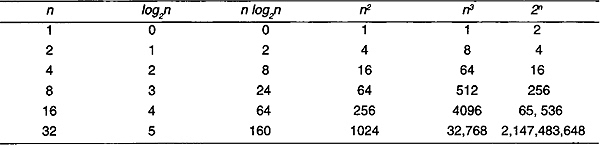
Note that O(n log n) is better than O(n2) but not as good as O(n). Similarly, if an algorithm takes time O(log n) it is faster, for sufficiently large n, than if it had taken O(n).
For reasonably large problems we always want to select algorithms of the lowest order possible. If algorithm A is O[f(n)] and B is O[g(n)], then algorithm A is lower order than B if f(n)< g(n) for all n greater than same constant K. For example, O(n2) is lower order than O(n3) because n2<n3 for all n>1. Similarly, O(n3) is lower order than O(2n) since n3<2n for all n >9.
Thus we would definitely want to select an O(n2) algorithm to solve a problem, instead of an O(n3) or O(2n) algorithm, if such an O(n2) algorithm existed.
Fig. 2.11 shows the behaviour for algorithms of orderO(2n), O(n3/2), O(5n2), and O(l00n).
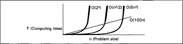
Fig. 2.11 Comparison of four complexity measures O(2n), O(n3/2), O(5n2) and O(100n)
This type of analysis provides the general guidelines we need and thus O notation is the fundamental technique for describing the efficiency properties of algorithms.
One important system of description used throughout the book is the use of notation of the form 0[f(n)] to describe the time or space requirements of running algorithms. If n is a parameter that features the size of the input to a given algorithm, and if we say the algorithm runs to completion in O[f(n)] steps, we mean that the actual number of steps executed is no more than a constant time f(n) for sufficiently large n.
2.5.2 Space Complexity
In space complexity, we need to develop a formula that relates n, the problem size, to s, the amount of memory space needed to solve the problem. For example, if an algorithm requires a table large enought to hold all n items, the space complexity is of the order O(n). For inputs of size n<20, the program with running time 5n3 will be faster than the one with running time 100n2. So if the program is to be run mainly on inputs of small size, we would prefer the program whose running time was O(n3). When n is large, that is, the size of the input increases, the O(n3) program will take significantly more time than the O(n2) program. Both the sequential and the binary search (to be discussed in sorting and searching chapter) methods require a table large enough to hold all n items and are therefore O(n) in terms of space complexity.
Memory space is inversely proportional to computer time. So we can frequently reduce space requirements by increasing processing time or conversely reduce processing time by making more memory available. This situation is referred to as space-time trade-off. For example, when we store the elements of an n x n array we need n2 memory locations. If most of the array elements are zero then reduction of space is possible in exchange of additional time for storing elements in reduced representation. It is always a challenge for computer scientists to find algorithms that solve give types of problems with the lowest possible complexity class for time space. So in this book, the discussion and comparison of algorithms for data structures and space consumed by data representation often comments on the complexity class O[f(n)] characterizing the time and space resources required.
2.6 STRUCTURED PROGRAMMING
The logic of any program can be developed entirely in terms of three types of logic structures: sequence, selection, and iteration. These logic structures are called the elementary building blocks and have one key feature in common, namely, a single entry point and a single exit point. A structured program is one consisting entirely of these elementary building blocks. These structures are sufficient to express any desired logic.
The theoretical framework for structured programming was initially presented at an International Colloquium in Israel in 1964. The authors, Bohm and Jacopini, presented their work in Italian and were essentially ignored in the United States. The english translation of their paper, published in 1966 in Communications of the ACM, did not gain a great deal of attention because of its theoretical nature. In 1968, a letter was sent to the editor by Edger W. Dijkstra of the Netherlands. In this letter, he wrote that ‘the quality of programrs is a decreasing function of the GOTO statements in the programs they produce.’ He further suggested that ‘the GOTO statement should be abolished from all high level programming languages…. it is an invitation to make a mess of one's program.’
Bohm and Jacopini had proved it theoretically that a program can be written without GOTO statements. Hartlan Mills and F Terry Baker, two Americans, demonstrate the practical aspects of the then revolutionary technique.
Structured programming techniques began to appear with greater frequency in the middle and late 1970s. The development was spurred considerably by the widespread introduction of Edward Yourdon's seminars on the subject. Today it is safe to say that virtually all practitioners atleast acknowledge the merits of the discipline, and most practice it exclusively.
Three elementary building blocks are depicted in Fig. 2.13. The sequence structure formally specifies that program statements are executed sequentially, in the order in which they appear. The two blocks, x, and y, may denote anything from single statements to complete programs.
Selection, also known as IF THEN ELSE, is the choice between two actions. If the condition is satisfied, block x is executed. If it is not satisfied, block y is executed. The condition is a single entry point to the structures, and both paths meet in a single exit point.
Iteration (also known as DO WHILE) calls for repeated execution of code while a condition is true. The condition is tested. If it is true, block x is executed; if it is false, the next sequence of statements will be executed.
Let us look again at the significance of the building block concept of Bohm and Jacopini. A block can consist of only one statement, or it can consist of a sequence of single statements, or it can contain of other blocks that in turn contain other blocks as a part of their structures. The structure is called nested control structure. A nested structure is shown in Fig. 2.12. A program or module can be built up in this way. The program itself can then be viewed as a single structure. A program having only one entry point and one exit point, and in which, for every structure, there exists a path from entry to exit, the program which includes it is called a proper program.
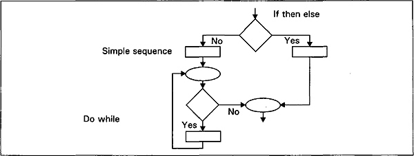
Fig. 2.12 Nested control structures
Structure relinquishes control to the next sequential statement. Again, there is one entry point and one exit point from the structure.
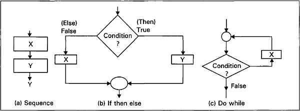
Fig. 2.13 The building blocks of structural programming
Consider again Fig. 2.12. The entry point to Fig. 2.12 is a selection structure to evaluate the condition. If the condition is false, an iteration structure is entered. If the condition is true, a sequence structure is executed. Both the iteration and sequence structure meet at a single point, which in turn becomes the exit point for the initial selection structure.
We have acquired some familiarity with the basic patterns, which are sufficient for any program. Certain other combinations have proven to be especially useful. One is the combination of simple sequence and do-while, known as do-until control structure. Even though the nested if-then-else structure seems to be useful for any number of conditions, it is difficult to draw such a flowchart or pseudocode. Case structure is a generalization of the nested if then else pattern with a large number of possible conditions. These two structures are shown in Fig. 2.14.
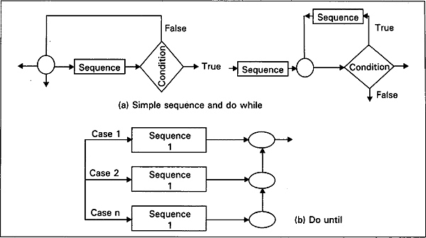
Fig. 2.14 The logic of case structure and logic of do-until
In this section, we have used ANSI standard flowcharting symbols within the structure of visualizing the program login set up within the structured programming control structures. Some feel that the structural programming is self-explanatory and need not be accompanied by flowcharts. These persons usually point out that a flowchart often fails to represent the current status of a program. To many, the use of pseudocode is a viable alternative to flowcharting. It permits the programr to express required program logic unencumbered by programming language rules and constraints.
After a structured program has been designed, it must be expressed in a programming language which supports the structured construct. The primary language statements directly analogous to the control structures we have described are available in a particular language. C language supports these constructs. In the next chapter, array as a data structure will be introduced.
E![]() X
X![]() E
E![]() R
R![]() C
C![]() I
I![]() S
S![]() E
E![]() S
S
1. A function ex can be approximated by using the following formula:
ex= 1 + x + x2 /2! + x3 /3! +…+ xk /k!
Write an algorithm for finding ex, where x is given as input.
2. What is the smallest value of n such that an algorithm whose running time is 100n2 runs faster than an algorithm whose running time is 2n on the same machine?
3. The most common computing times for algorithms are:
O (1)
O (log2n)
O (n)
O (n log2 n)
O (n2)
O (n3)
O (2n)
Draw a graph for their time complexities in the range 1≤ n ≤128 and compare their rate of growth.
4. Compare the two functions n2 and 2n/4 for various values of n. Determine when the second becomes larger than the first.
5. Given n, a positive integer, determine if n is the sum of all of its divisors; that is, if n is the sum of all t such that 1≤ t ≤ n and t divides n. Draw a flowchart for this problem.
6. Write pseudocode for the insertion sort to sort into nonincreasing instead of nondecreasing order.
7. What are the main advantages of a decision table over a flowchart?
8. Discuss the merits and demerits of top-down and bottom-up approaches to algorithm design.
9. Imagine that we have an algorithm p whose time complexity we have analyzed and found to be O [log2(log2n)]. What would be the position of that complexity function in the ordered list of functions given in Exercise 3?
10. Can we write a O(1) algorithm to determine n! for 1≤ n ≤15?