
Chapter 10
Three-dimensional Systems
10.1 INTRODUCTION
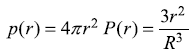
In Chapter 5, we discussed time-independent Schrodinger equation for a particle in various one-dimensional potentials. In this chapter, we shall discuss the structure of the Schrodinger equation and solve it for a particle moving in a (time-independent) three-dimensional potential V(r) for which the technique of separation of variables may be used. In such cases, the original three-dimensional problem reduces to simpler (one-dimensional) problems. We shall start our discussion with the study of a free particle in three-dimensional space. Then we shall discuss motion of a particle in spherically symmetric potentials V(r) (which depend only upon the magnitude r = |r|), like attractive Coulomb potential [V(r) = – (Ze2)/4π∊οr] and spherical harmonic potential ![]()
10.2 A PARTICLE IN A CUBIC POTENTIAL BOX
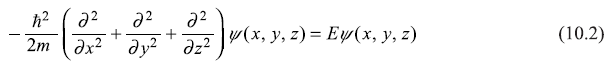
Let a particle of mass m be confined in a cubic potential box of side L. Inside the box the potential V is a constant which we may take to be zero, while at and outside the walls V is infinite. The potential box shown in Figure 10.1 is defined as
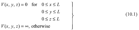
The time-independent Schrodinger equation of the particle inside the box is
The form of this equation suggests that the wave function ψ(x, y, z) may be expressed as product of three functions, each of a single variable.
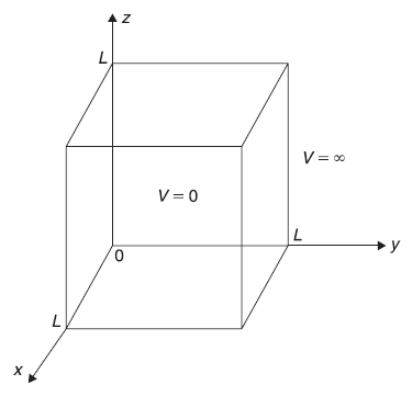
Figure 10.1 Cubic potential box
Substituting (10.3) into (10.2) and dividing both sides by ψ, one finds

Each of the expressions in the three square brackets, is a function of only one of the variables x, y, z. The sum of these expressions is equal to the constant E. Therefore, each expression should itself be equal to a constant; let three constants be E1, E2 and E3. So, we get three differential equations.
with
Each of the above differential equations (10.5) has the form of a one-dimensional Schrodinger equation (5.24) of Chapter – 5, and can be solved the way (5.24) was solved.
For the particle being confined within the box of infinite potential at the walls, the wave function ψ(x, y, z) must vanish at each of the walls and beyond. This, so called rigid boundary condition, may be expressed in the form
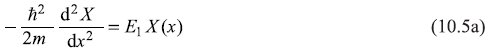
On the basis of the results of Section (5.4), the solutions of equation (10.5a) (i.e. the allowed energy eigenvalues Enx and corresponding normalised eigenstates Xnx(x) may be written as
where
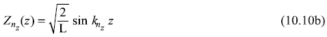
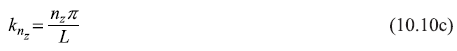
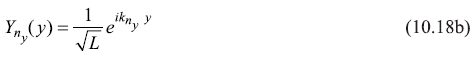
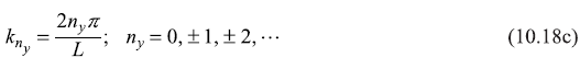
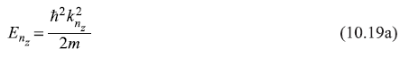
Similar expressions may be written for energy eigenvalues and eigenfunctions of equations (10.5b) and (10.5c) [i.e. for Eny, Yny (y) and for Enz, Znz (z)]
with
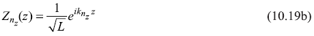
and
with
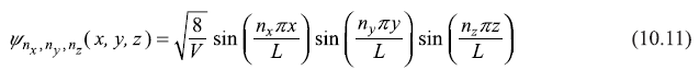
We can now write the normalised eigenfunctions of the full three-dimensional system as
and the allowed values of energy E = Ex + Ey + Ez as
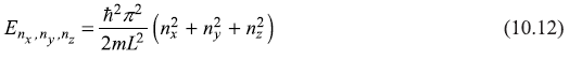
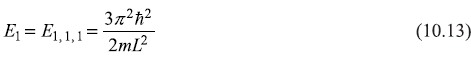
The ground state energy E1 corresponds to nx = ny = nz = 1
There is only one state ψ1, 1, 1 which has energy E1, so this level is non-degenerate. The next energy level corresponding to the set of quantum numbers nx = 2, ny = 1, nz = 1, has energy (6π2ħ2/2mL2) = 2 E1. But the set (nx, ny, nz) with values (1, 2, 1) and (1, 1, 2) also give energy 2E1. Therefore this level is three-fold degenerate: states ψ2, 1, 1, ψ1, 2, 1 and ψ1, 1, 2 have same energy 2E1. The next energy levels and the corresponding degeneracies may be obtained in a similar way. In Figure 10.2, we show first few energy levels alongwith their degeneracies.
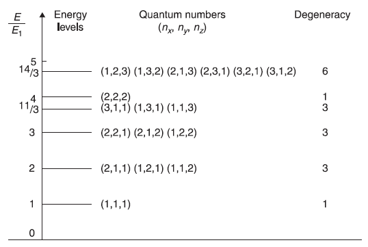
Figure 10.2 First few energy levels of a particle in a cubic potential box (under rigid boundary conditions). Also shown are the quantum numbers (nx, ny, nz) and the degeneracy of each energy level. The energy is expressed in terms of ground state energy E1 = 3ħ2π2/2mL2
10.3 CUBIC BOX WITH PERIODIC BOUNDARY CONDITIONS
In Section 10.2 we discussed the energy eigenvalues and eigenstates of a particle in a three-dimensional box under rigid boundary conditions. If we consider electrons in conduction band in a (simple) metal, we generally encounter a model called as “free electron model” of conduction band in metals (the Sommerfield Model). In this model electrons are treated as freely moving particles inside the metal. In fact, this is an approximation which may be valid in some cases. In some metals the net potential of all positive ions (sitting at lattice points) and of all other conduction electrons on a test electron is really very weakly varying (in space) which, as a first approximation may be taken to be constant (or zero). Thus with this approximation, all electrons (of conduction band) move freely inside metal. That simply means, an electron is moving in the metal as if all other electrons and positive ions are not present there. So our present study of finding energy eigenvalue and eigenfunctions of a particle in a three-dimensional box should be applicable to the electrons in metals.
In last section we considered a particle in a box under rigid boundary conditions, where eigenstates are the standing waves [given by equation (10.11)]. Now, these standing waves do not carry linear momentum i.e.
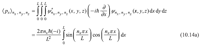
So these standing waves (which are the correct eigenstates of a particle in a box under rigid boundary conditions) are really of no help in problems of electrical conductivity in metals, for which we should require running waves of electrons or wave functions which describe the motion of an electron in a definite direction. Also when we discuss any electronic property of a metal (e.g. electrical conductivity, electronic specific heat etc.) we hardly mention shape or size of the metal. Therefore we would like to have description of electrons in a metal, which does not include surface or boundary effects. There is an elegant mathematical trick to achieve this goal. We shall have to simply get rid of the rigid boundary conditions, and shall have to use periodic boundary conditions. In fact, we had already used periodic boundary conditions in the one-dimensional potential box case (Section 5.5). And there we found the eigenstates to be propagating waves.
The periodic boundary conditions for three-dimensional box may be expressed as
So now Schrodinger equation (10.2) is to be solved with periodic boundary conditions (10.15). Expressing the wave function ψ(x, y, z) as product of three functions, each of a single variable, just like in equation (10.3), we need to solve equations (10.5) with periodic boundary conditions.
In Figure 10.3 we illustrate the periodic boundary conditions applied to one-dimensional wave function.
Based on the results of Section (5.5), the solution of equation (10.5a) for the boundary condition (10.16a) may be written as
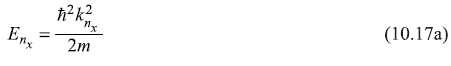
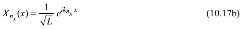
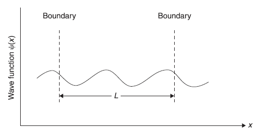
Figure 10.3 Illustration of periodic boundary conditions applied to one-dimensional wave function ψ(x) in such a way that ψ(x + L) = ψ(x)
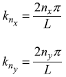
with
Similarly, expressions may be written for energy eigenvalues and eigenstates of equations (10.5b) and (10.5c).
with
and
with
The resulting (normalised) eigenstate may be written as
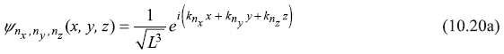
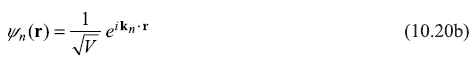
or
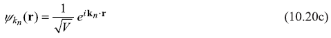
and energy eigenvalues are given as
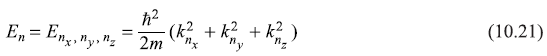
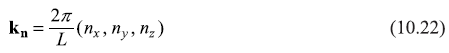
where n denotes the set of integers {nx, ny, nz}, kn is wave vector having components knx, knx, knz and r is the position vector. The allowed values of wave vector kn are
In Figure 10.4, we show first few energy levels [given by Eq. (10.21)] alongwith their degeneracies. In Figure 10.5, we show by dots the allowed k-values in k-space.
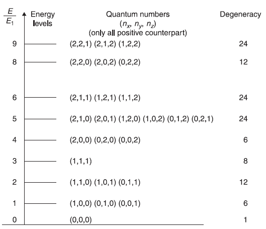
Figure 10.4 First few energy levels of a particle in a cubic potential box (under periodic boundary conditions). Also shown are the quantum numbers (nx, ny, nz) (only all positive counterpart). Last column shows the degeneracy of each energy level. The energy is expressed in terms of the energy of first excited state E1 = ħ2π2/2mL2
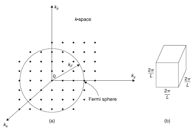
Figure 10.5 (a) Allowed k-points in three-dimensional k-space. Also shown is the spherical Fermi surface (of radius kF) with Fermi energy EF (b) The volume of k-space occupied by one k-state is [2π/L]3
10.4 DENSITY OF STATES OF FREE PARTICLES (FREE ELECTRON GAS IN METALS)
As mentioned in Section 10.3, electrons in the conduction band of some metals move almost freely inside the metal. Sommerfield model treats these electrons to be totally free and this model works very well in simple metals. We have seen that use of periodic boundary conditions for a particle in a box gives eigenstates which are plane propagating waves. Therefore we visualise the free (non-interacting) electrons in metals just like (non-interacting) particles in a potential box with periodic boundary conditions.
We know in metals, there are of the order of 1022 atoms in one cubic centimeter (c.c.). And if each atom contributes one electron to the conduction band, there are around 1022 electrons per c.c. The electrons, being fermions, follow Pauli’s exclusion principle. Therefore, 1022 electrons shall occupy 0.5 × 10²² quantum states in the ground state of metal. The energy of the highest occupied level is called as Fermi energy. It is observed experimentally that Fermi energy of simple metals is of the order of a few electron volts (eV). So there are around 1022 quantum states within an energy span of few electron volts. This implies that energy separation between two consecutive quantum levels is really very small: of the order of 10–21eV. Therefore, though the energy levels are discrete, these are very densely packed (in energy space). Naturally, it will be very relevant (and useful) to talk in terms of the density of (these quantum) states.
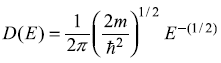
The definition of the density of states is analogous to the definition of other densities (like particle number density n being the number of particles in unit volume). So the density of states D(E) is the number of (quantum) states in unit energy interval around energy E. And therefore, D(E) dE is the number of states lying in between energies E and E + dE.
10.4.1 Density of States in One-dimensional Case
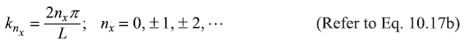
For an electron in a one-dimensional metal (i.e. an electron in a one-dimensional potential box with periodic boundary conditions), the energy eigenvalues are given by
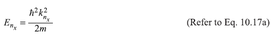
with
In Figure 10.6 we plot the relation (10.17a) and show the allowed values of energy E and wave vector k. Let us choose two points k and k + dk on k-axis. Let the corresponding energies be E and E + dE. If the density of states at energy E is D(E), the number of energy states in between E and E + dE is D(E) dE. And this number of states should be equal to the number of k-points in the interval k and k + dk plus those in the interval –k and –k –dk.
Here D(k) is the density of k-points at wave vector k, given by
From Eq. (10.23)
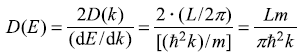
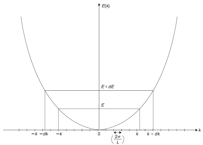
Figure 10.6 E versus k curve in one-dimensional case. Also shown are allowed k-points. Length of k-space occupied by one k-point is (2π/L).
Often one sets the length L = 1, so
10.4.2 Density of States in Two-dimensional Case
For an electron in a two-dimensional box, energy eigenvalues are given by
with knx and kny given by equations (10.17c) and (10.18c) respectively. In Figure 10.7, we show allowed k-points in the two-dimensional k-space. The number of k-points lying in the annular ring of inner radius k and outer radius k + dk is equal to D(k) 2πk dk, where D(k) is the density of k-points, given by
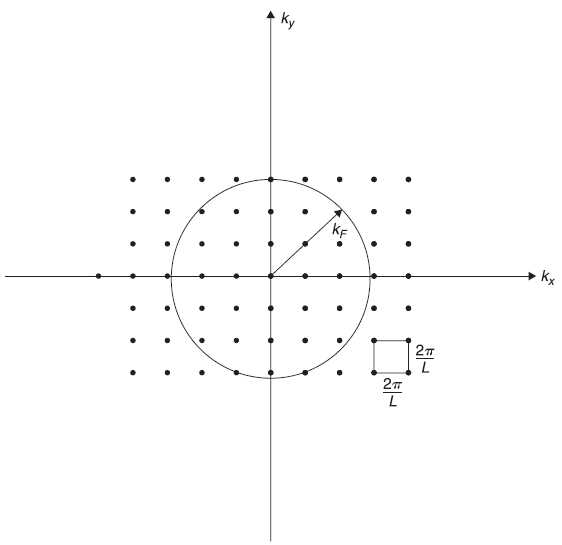
Figure 10.7 Allowed k-points in two-dimensional k-space. Area of k-space occupied byone k-point is (2π/L)2. Also shown is a circle having all k-points on it of same energy
Let E and E + dE be the energies corresponding to wave vectors k and k + dk. Then the number of states in the interval E and E + dE is equal to the number of k-points lying in the annular ring of radii k and k + dk, that is
or
For

10.4.3 Density of States in Three-dimensional Case
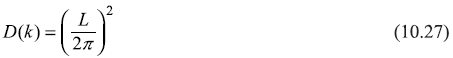
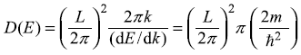
For an electron in a three-dimensional box the energy eigenvalues are given by equation (10.21) with allowed values of knx, kny, knz given by equations (10.17c), (10.18c) and (10.19c) respectively. Figure 10.5 shows allowed k-points in three-dimensional k-space. Let us consider a spherical shell centred at the origin, of inner and outer radii k and k + dk respectively. The number of k-points in this spherical shell is D(k)4πk2 dk, where the density of k-points D(k) is given by

So,
or
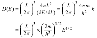
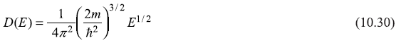
For
In Figure 10.8 we show schematic plots of density of states for one-, two-, and three-dimensional cases.
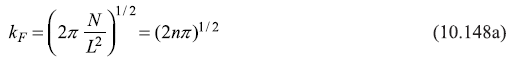
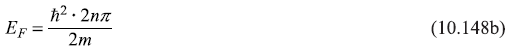
Let us now consider free electron gas in three-dimensions at temperature T = 0K. The energy levels are given by Eq. (10.21). With N electrons (in the box of volume V) we start filling states from the bottom by putting two electrons (one of spin up and one of spin down) in each state. Let the highest occupied level be of energy EF (and of wave vector kF). The energy EF and wave vector kF are known as
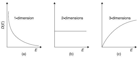
Figure 10.8 Variation of density of states (schematic) for (a) one-dimensional (b) two-dimensional and (c) three-dimensional cases
Fermi energy and Fermi wave vector, respectively. All k-states within the sphere of radius kF are occupied. This sphere is known as Fermi sphere. In Figure 10.5(a), we show Fermi sphere. Now
or
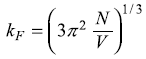
where n = N/V is the electron number density.
Using the relation
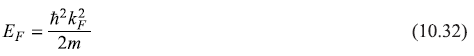
We get
It may be noted that both, the Fermi energy EF and the Fermi wave vector kF depend only on electron number density n (= N/V). Also we can easily find out the Fermi velocity vF, the velocity of electrons at the Fermi surface. It is given as
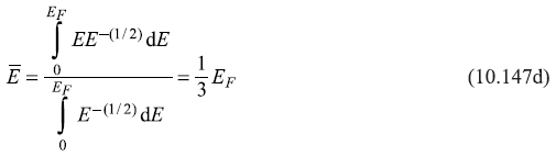
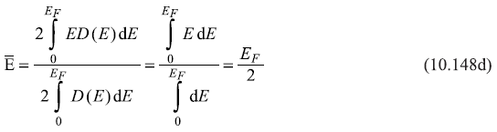
One notices here that all N electrons (in volume V) are occupying energy levels from zero to EF; two electrons in each state. We may easily calculate the average energy of an electron in the following way
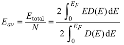
Using equation (10.30) for D(E), one gets
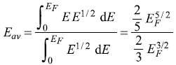
or
So even at T = 0K, the average (kinetic) energy per electron is ![]() EF. The Fermi energy in simple metals is a few electron volts. Therefore average kinetic energy of an electron in conduction band of simple metals, even at T = 0K, is a few electron volts. If electrons were behaving like classical particles and therefore there were no Pauli exclusion principle for them, all the electrons would have come to zero kinetic energy state at T = 0K. Therefore the notion that at absolute zero temperature, the kinetic energy of particles of the system shall become zero, is not correct. At least it is not true for quantum particles.
EF. The Fermi energy in simple metals is a few electron volts. Therefore average kinetic energy of an electron in conduction band of simple metals, even at T = 0K, is a few electron volts. If electrons were behaving like classical particles and therefore there were no Pauli exclusion principle for them, all the electrons would have come to zero kinetic energy state at T = 0K. Therefore the notion that at absolute zero temperature, the kinetic energy of particles of the system shall become zero, is not correct. At least it is not true for quantum particles.
10.4.4 An Alternate Method of Finding Density of States
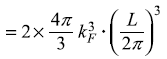
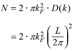
Let us revisit the case of quantum levels of three-dimensional electron gas, discussed in sub-section (10.4.3). Let us find out total number of states, N, upto energy E [or upto wave vector ![]() . The total number of states upto wave vector k, i.e. total number of states in the sphere of radius k (in k– space) are given as
. The total number of states upto wave vector k, i.e. total number of states in the sphere of radius k (in k– space) are given as
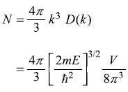
or
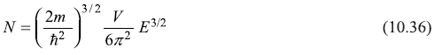
Now,
as dN = D(E) dE is nothing but the number of states in between E and E + dE.
∴
for V = 1, it is same as equation (10.30).
10.5 SPHERICALLY SYMMETRIC POTENTIALS
We now turn to the study of the motion of a particle in a potential V(r) which depends only on the magnitude r of the position vector r of the particle. Such potential may be referred to as a spherically symmetric potential. We shall see that the properties of the orbital angular momentum L = r × p studied in Chapter 9 are of particular importance in the present context.
Since the potential V(r) we are considering is spherically symmetric, it will be very convenient to use spherical polar coordinates here. Let us express the Hamiltonian operator in polar coordinates as
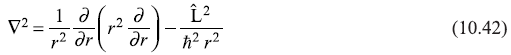
where operator ∇2 is expressed as
We know from Chapter – 9 that the orbital angular momentum operator ![]() is given by
is given by
Therefore, ∇2 may be written as
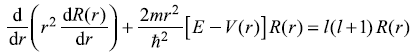
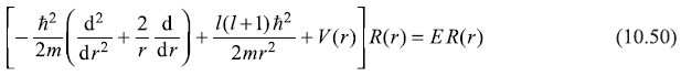
So the three-dimensional, time-independent Schrondinger equation of a particle in a potential V(r) may be written as
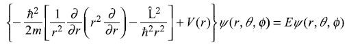
or

Let us recall from Chapter 9 that the orbital angular momentum operators ![]() and
and ![]() do not contain the radial variable r [see Eqs. (9.18) and (9.19)]. Therefore, for a spherically symmetric potential V(r), we have
do not contain the radial variable r [see Eqs. (9.18) and (9.19)]. Therefore, for a spherically symmetric potential V(r), we have
Now the kinetic energy operator ![]() is given as
is given as
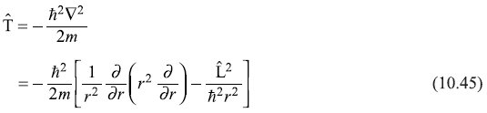
[using equation (10.42)].
It can be easily seen that the operators ![]() and
and ![]() also commute with operator
also commute with operator ![]() . Therefore
. Therefore
We know that operators ![]() do not commute among themselves but each one commutes with
do not commute among themselves but each one commutes with ![]() . Therefore a set of commuting operators may be taken as H,
. Therefore a set of commuting operators may be taken as H, ![]() and any one of
and any one of ![]() and
and ![]() . Let us take this set to be
. Let us take this set to be ![]() . As property of commuting operators, it is possible to find simultaneous eigenfunctions of these (three) operators. In other words we may say, it is possible to obtain solutions (i.e. eigenstates) of the Schrodinger equation (10.43) which are also eigenstates of operators
. As property of commuting operators, it is possible to find simultaneous eigenfunctions of these (three) operators. In other words we may say, it is possible to obtain solutions (i.e. eigenstates) of the Schrodinger equation (10.43) which are also eigenstates of operators ![]() and
and ![]() . In Chapter 9 we saw that the spherical harmonics Yl, m (θ, ϕ) are simultaneous eigenstates of
. In Chapter 9 we saw that the spherical harmonics Yl, m (θ, ϕ) are simultaneous eigenstates of ![]() and
and ![]() . Therefore the solutions of the Schrodinger equation may be expressed in the separable form
. Therefore the solutions of the Schrodinger equation may be expressed in the separable form
Substituting (10.47) in (10.43), one gets
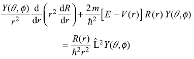
Dividing both sides by R(r)Y(θ,ϕ)/r2, we get

Here the L.H.S. depends only on r and R.H.S. depends on θ and ϕ, therefore each should be equal to a constant, say λ. The eigenvalue equation of operator ![]() becomes
becomes
and we know from the results of Chapter 9 that operator ![]() has eigenvalues as l(l + 1) ħ2 and corresponding eigenstates as spherical harmonics Yl, m (θ, ϕ). So constant λ in Eq. (10.48) is l(l + 1). Thus equation (10.48) gives the following equation for the radial part R(r):
has eigenvalues as l(l + 1) ħ2 and corresponding eigenstates as spherical harmonics Yl, m (θ, ϕ). So constant λ in Eq. (10.48) is l(l + 1). Thus equation (10.48) gives the following equation for the radial part R(r):
or
Let us introduce the new radial function
We obtain the radial equation for u(r) as

where
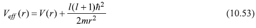
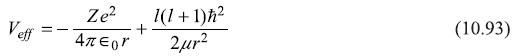
Equation (10.52) is a one-dimensional Schrodinger equation of a particle in an effective potential Veff (r) which, in addition to the interaction potential V(r), also has the repulsive centrifugal barrier term [l(l + 1)ħ2 / 2mr2].
10.6 THE FREE PARTICLE IN SPHERICAL POLAR COORDINATES
The Schrodinger equation for the radial part R(r) of the wave function of a particle in a central potential V(r) is given by Eq. (10.50). We may consider the simple case of a free particle here, for which V(r) = 0. We have already solved Schrodinger equation of a free particle in cartesian coordinate system, and obtained plane wave solutions in Section (10.3). These plane wave states are also linear momentum eigenstates as free particle Hamiltonian operator ![]() ∇2 commutes with the linear momentum operator
∇2 commutes with the linear momentum operator ![]() . Now using spherical polar coordinates, we look for the solutions of the free particle Schrodinger equation, of the form (10.47). In fact the eigenstates like (10.47) of the Hamiltonian of a particle in a central potential (or that of a free particle) are also the eigenstates of angular momentum operators
. Now using spherical polar coordinates, we look for the solutions of the free particle Schrodinger equation, of the form (10.47). In fact the eigenstates like (10.47) of the Hamiltonian of a particle in a central potential (or that of a free particle) are also the eigenstates of angular momentum operators ![]() and
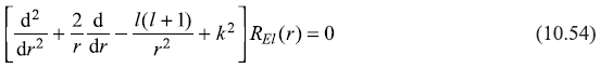
and ![]() . For a free particle the radial function REl(r) are the solutions of the radial equation (10.50) with V(r) = 0, re-written as
. For a free particle the radial function REl(r) are the solutions of the radial equation (10.50) with V(r) = 0, re-written as
where
Introducing the new radial function, just like that in Eq. (10.51), uEl(r) = rREl(r), we get the radial equation for uEl(r) as
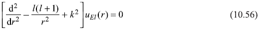
Now for the case l = 0, above equation gives the solution uEl(r) = A sin kr or A cos kr. But REl(r) = [uEl(r)]/r has to be finite at r = 0, therefore the only solution, admissible, is
which gives for l = 0,
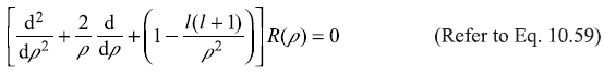
For l ≠ 0, let us rewrite Eq. (10.54) in changed variable ρ = kr as
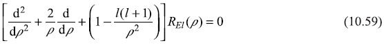
This is called the spherical Bessel Differential equation. For l = 0, 1, 2, ... the particular solutions of this equation are the spherical Bessel functions
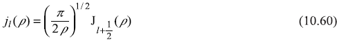
and the spherical Neumann functions
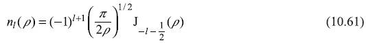
where Jv(ρ) is an ordinary Bessel function of order v.
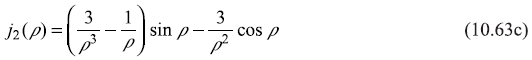
It may be checked that the following expressions of jl(ρ) and nl(ρ) satisfy Eq. (10.59).
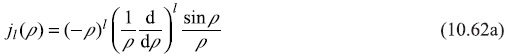
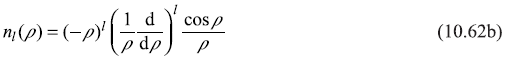
From these equations, one may easily find a few functions jl(ρ) and nl(ρ):


The asymptotic forms of jl(ρ) and nl(ρ) are
10.6.1 The Eigenstates of Free Particle
It can be noted that the spherical Bessel function jl(ρ) is finite at ρ = 0, whereas nl(ρ) diverges at ρ = 0. Therefore, jl(ρ), which is finite for all values of ρ, is a regular solution of Eq. (10.59). The Schrodinger equation (10.54), for a free particle, thus has radial eigenstate given by
As asymptotic form of jl(kr) is sin (kr – lπ/2)/kr which has the form of a spherical wave (as can be seen by adding time part of it), the wave functions (10.67) are called spherical waves.
10.6.2 Expansion of Plane Waves in Spherical Harmonics
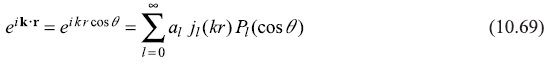
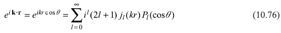
It may be mentioned here that we have two alternative complete sets of eigenstates of the free particle Hamiltonian. Firstly, we have the complete set of plane waves eik.r (Section 10.3) and secondly, there are complete set of spherical waves jl(kr) Yl, m(θ, ϕ). In fact these two sets of eigenstates are equivalent and an eigenstate of one set should be capable of expanding in terms of the other set. For example, we may have plane wave expansion as
where coefficients al,m are to be determined. Let us consider the case where k lies along z-axis. Then the left hand side of Eq. (10.68) eik.r = eikr cosθ, is independent of ϕ, so its expansion reduces to that in terms of Legendre polynomials Pl(cosθ). Therefore,
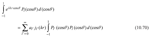
Multiplying both sides of above equation by Pl(cosθ) and integrating, we get
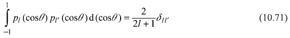
Using the orthogonality relations of the Legendre polynomials
Equation (10.70) gives
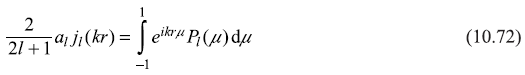
where µ = cos θ. Integrating it by parts, gives
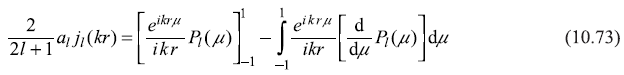
Let us consider this equation in the limit r → ∞. We get (neglecting second term on right side, which comes out to be of order 1/r2)
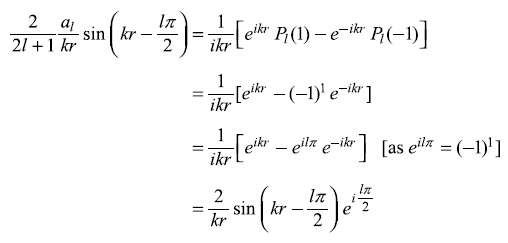
or
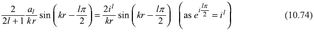
which gives
Substituting this in Eq. (10.69), one gets
10.7 SCHRODINGER EQUATION FOR A TWO-BODY SYSTEM
In the next Section we shall discuss Schrodinger equation for a hydrogen-like atom, as an example of spherically symmetric potential. In this Section we consider a general case of two particles of masses m1 and m2, interacting with a time-independent potential V(|r1 – r2|); the potential depending only on the magnitude of the distance between the two particles. We shall see that in such a case the problem always reduces to a one-body problem alongwith a uniform translational motion of the centre of mass of the two-particle system.
The Hamiltonian of the two particle system is given by
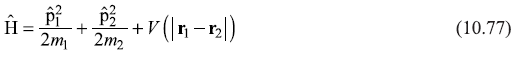
Now with the substitution of operator form ![]() and
and ![]() , the corresponding time-independent Schrodinger equation is
, the corresponding time-independent Schrodinger equation is
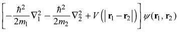
This is a six-dimensional partial differential equation. The potential energy function V(|r1 – r2|) cannot be written as the sum of two functions, one in variable r1 and the other in r2. Therefore it is not possible to write equation (10.78) as sum of functions in separate variables. However, if we introduce the relative coordinate
and the centre of mass coordinate
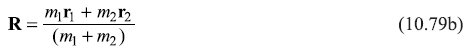
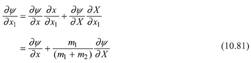
it is possible to write equation (10.78) in terms of functions in separate variables. Let us write x-components of r and R from (10.79).
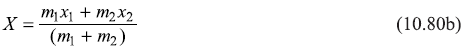
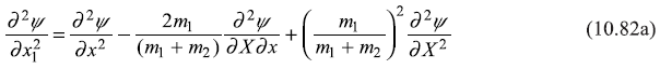
Similarly, y- and z-components may be expressed. Now
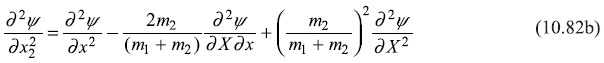
and
Similarly, one may get
Therefore,
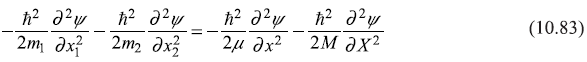
where
is the total mass of the system and
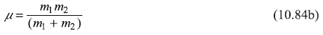
is the reduced mass of two particle system.
With the help of equation (10.83) (and with similar equations in y- and z-variables) Schrodinger equation (10.78) may be written as
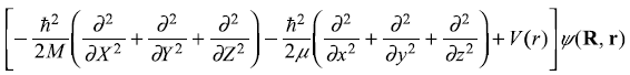
or
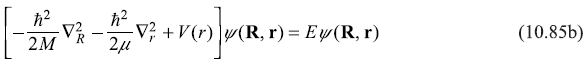
It is straightforward to check that this equation (10.85b) may be obtained, alternatively, by introducing the relative momentum.
and the total momentum
One may easily check that equations (10.86) give
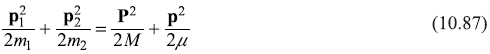
So, the Hamiltonian becomes
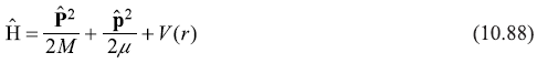
and with the substitution ![]() and
and ![]() in (10.88), one gets the Schrodinger equation (10.85b). By writing
in (10.88), one gets the Schrodinger equation (10.85b). By writing
it is easy to see that equation (10.85b) is now separable, giving following two equations
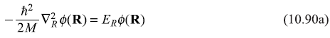
and
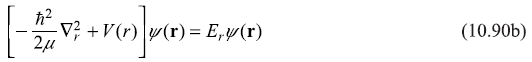
with
Equation (10.90a) describes the centre of mass as a free particle of mass M and energy ER. Equation (10.90b) describes the relative motion of two particles. In fact, (10.90b) is the equation corresponding to the motion of a particle having the (reduced) mass µ in the potential V(r). Therefore, if we work in a frame of reference in which the centre of mass is fixed, we are only left with the discussion of a single particle of (reduced) mass µ in potential V(r).
10.8 THE HYDROGENIC ATOM
As an example of spherically symmetric potential, let us consider a hydrogen – like atom i.e. one electron atom with a nucleus of charge Ze. The potential energy of electron V(r) is
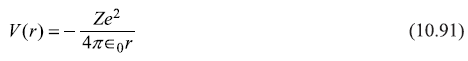
Here Z = 1 for hydrogen atom, Z = 2 for He+, Z = 3 for Li++ etc. So to find out energy eigenvalues and eigenstates of the electron we shall have to solve the radial equation (10.50) with potential V(r) given by equation (10.91). Let us re-write this equation below:
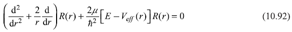
where
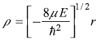
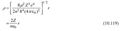
We are interested in solving equation (10.92) for bound states of electron i.e. for energy E < 0. Let us introduce the (dimensionless) quantities.
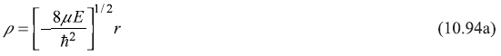
and
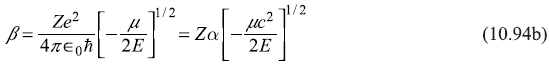
where
is the fine structure constant. Equation (10.92) now becomes
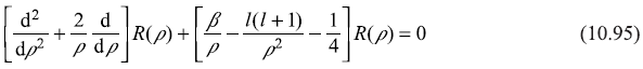
Now let us firstly look at the asymptotic behaviour of radial function R(ρ). For ρ → ∞, equation (10.95) reduces to
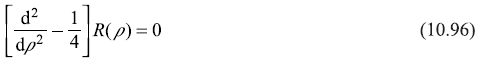
The solutions to this equation are
But as the function R(ρ) should be finite everywhere, R(ρ) should have only exponentially decreasing form. Therefore
This suggests that the radial equation (10.95) should have solutions of the form
Putting (10.98) into (10.95), we get

Let us write a series expansion for F(ρ) in the form
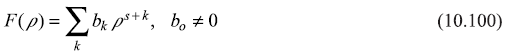
Inserting (10.100) into (10.99), we have
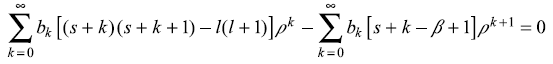
or
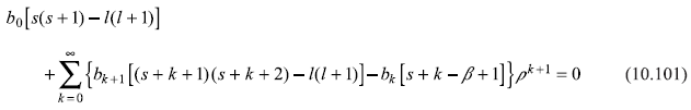
Since b0 ≠ 0, the quantity s must satisfy
so
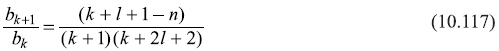
Now from equation (10.101) we obtain the recurrence relations

If we take s = –(l + 1), equation (10.103) gives
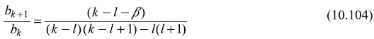
This equation indicates that one of the expansion coefficients becomes infinite (e.g. for k = 2l, the coefficient bk+1 becomes infinite) for the choice s = – (l + 1). Therefore we choose.
With this choice (10.100) and (10.103) give, respectively
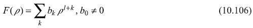
and
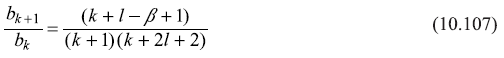
For large values of k, (10.107) gives
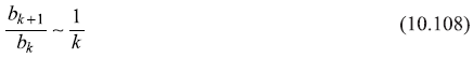
If we consider a function ϕ(ρ) = eρ, its series expansion is
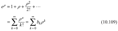
Thus the ratio of two consecutive coefficients is
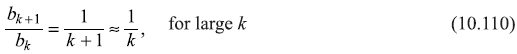
The ratio in (10.110) is same as that in (10.108). Thus, if the series (10.100) does not terminate, the asymptotic form of F(ρ) will behave as eρ. Using equation (10.98), R(ρ) will behave asymptotically like
So R(ρ) will diverge for ρ → ∞, unless the series for F(ρ), equation (10.106) terminates at some stage. The series may be terminated by requiring [in Eq. (10.107)].
With the condition (10.112), the coefficient bk+1 = 0 in (10.107). Now we know that l = 0, 1, 2, ... and also k = 0, 1, 2, ..., therefore n can have values 1, 2, 3, .... The number n is called as principle quantum number.
10.8.1 Energy Eigenvalues
From equation (10.94b) we have
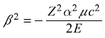
Putting β = n [Eq. (10.112)], we get

where
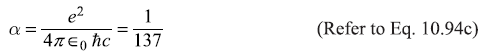
is the fine structure constant. Putting value of α in (10.113a), we get
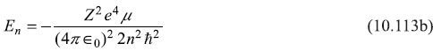
The Schrodinger equation for hydrogen atom gives energy eigenvalues (En) corresponding to various eigenstates of hydrogen atom. For hydrogen atom Z = 1, and putting values of all quantities in (10.113b), one gets
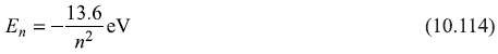
These values match exactly with the energy levels found from the Bohr model. However, the agreement of the energy spectrum based on (10.113b) does not match perfectly with the experimental spectrum. In fact, one will have to include various corrections/interactions not considered here (e.g. fine structure due to relativistic effects and due to electron spin, hyperfine structure due to nuclear effects). It may be noted from equation (10.113b) that energy eigenvalues En depend only on the principal quantum number n and not on quantum numbers l and m. In fact, it is clear from equation (10.112) that for a principal quantum number n, the orbital angular momentum quantum number l may take the values 0, 1, ... (n – 1). We also know from our study of angular momentum in Chapter-9 that for each value of l, the magnetic quantum number m may take the (2l + 1) possible values –l, –l + 1,..., l – 1, l. Therefore number of different quantum states corresponding to principal quantum number n is
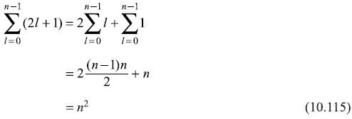
So for principal quantum number n, there are n2 different states having same energy eigenvalue En. These n2 different states are degenerate. We show energy levels of hydrogen atom in Figure 10.9.
10.8.2 The Radial Eigenfunctions
The radial eigenfunctions are generally denoted by Rnl(r) which, using equation (10.98) are expressed as
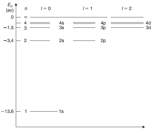
Figure 10.9 Energy levels of hydrogen atom
The expression for Fnj(ρ) is

The recursion relations for coefficients bk, with the termination requirement
become
To find out explicit expressions of Rnl(r) let us start with n = 1. For n = 1, the allowed value of quantum number l is only l = 0. From equation (10.112) we have n = k + 1. So only k = 0 term is there in the series (10.106). Therefore
which gives
We know the relation between ρ and r is
Now putting expression of energy from Eq. (10.113b), we get
where
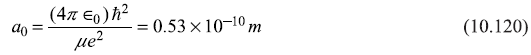
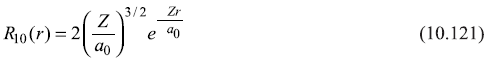
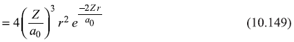
is the (first) Bohr radius of hydrogen atom. In terms of variable r, the eigenfunction (10.118) is written as
After normalizing, the eigenfunction is
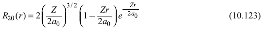
For n = 2, quantum number l has values l = 0, 1. With n = 2 and l = 0, recursion relation (10.117) suggests that b2 = 0. So only two terms with coefficients bo and b1 are there.
or
Therefore
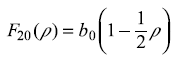
For n = 2, equation (10.119) gives ρ = (Zr/a0) and one can easily find the normalised eigenfunction R20(r) as
With n = 2 and l = 1, (10.117) suggests that b1 = 0, so the only term present there is with coefficient b0. Therefore
and normalised R21(r) may be written as
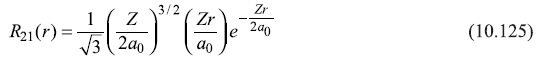
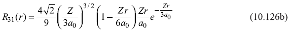
Proceeding in this way, one may easily find any required radial eigenfunction. We write below a few of these:
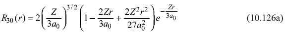
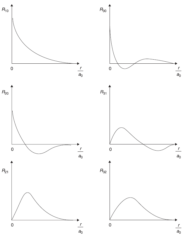
Figure 10.10 Schematic plot of Radial eigenfunctions Rnl(r) for hydrogen atom
In Figure 10.10 we illustrate these radial eigenfunctios schematically, for hydrogen atom.
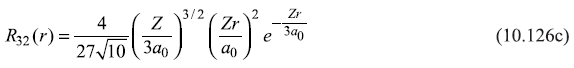
Below in Table 10.1 we write a few normalised hydrogenic wave functions ψn, m(r, θ, ϕ).
Table 10.1 The normalized hydrogenic wave functions ψnlm (r, θ, ϕ)
10.8.3 The Radial Probability Distribution Function
As discussed in Section 10.5, for spherically symmetric potentials the total wave function ψnlm(r, θ, ϕ) may be expressed as the product of the radial part Rnl(r) and the angular part (spherical harmonics) Ylm (θ, ϕ) [Eq. (10.47)]. We have displayed in Table 10.1 the normalised hydrogenic wave functions ψnlm(r, θ, ϕ) for few principal quantum numbers n = 1, 2, 3.
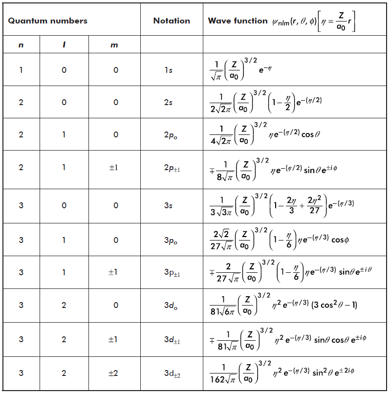
According to the Born’s statistical interpretation of the wave function ψ (discussed in detail in Chapter 3) the quantity
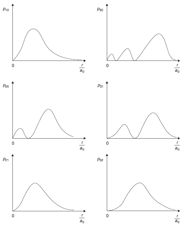
Figure 10.11 Schematic plots of few radial probability distribution function pnl(r), for hydrogen atom
represents the probability of finding the electron in the volume element dr around point r. (In spherical polar coordinates the volume element dr = r2dr sinθ dθ dϕ). When we express the wave function ψ in terms of its radial part and the angular part, we have
So |ψnlm(r, θ, ϕ)|2, describing the position propability density, does not depand on the coordinate ϕ. The position probability density is the product of the quantity |Rnl(r)|2 (which gives the electron density as a function of r along any direction) and of the angular part (1/2π)|Θlm(θ)|2. Now the probability of finding the electron in between r and r + dr irrespective of direction (θ, ϕ) (i.e. the probability of finding the electron in the spherical shell of inner and outer radii r and r + dr respectively) is
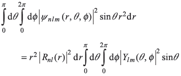
We call the quantity
as radial probability distribution function (or radial probability density). In Figure 10.11 we show schematic plots of the radial distribution functions for hydrogen atom.
EXERCISES
Exercise 10.1
The normalised wave function of an electron in a cubic potential box of side L nm is given as
Find out
- Value of side L
- wave vector components kx, ky, kz and quantum numbers nx, ny, nz
- energy of electron
- ψ(r, t)
- energy of the photon emitted when electron goes from state ψ(r, 0) to its next lower energy state.
- energy of electron when it is in ground state in this box.
The wave function of a free electron, normalised to the volume of a cubic box of side L, is given as
Find all quantities mentioned in above exercise.
Exercise 10.3
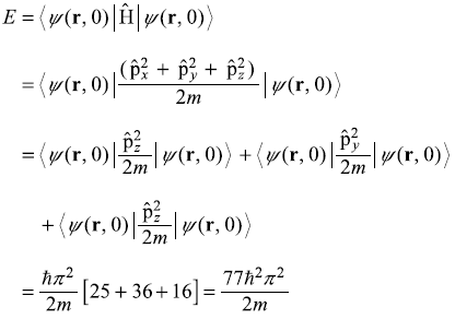
At time t = 0, a free particle is in the (normalised) state
Find out
- energy of the particle
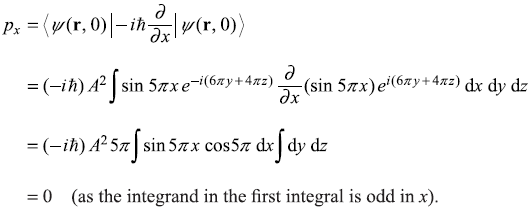
- values of linear momentum components px, py, pz of the particle.
- ψ(r, t)
- under what situations does a particle have a wave function like (10.133)?
Exercise 10.4
A particle is represented by the wave function
- Write the unit vector of the direction in which particle is moving.
- Find
- wave vector
- wavelength
- linear momentum
- angular frequency
- mass
- velocity
- (kinetic) energy
of the particle.
Exercise 10.5
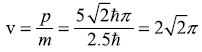
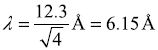
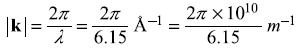
Write the time – dependent wavefunction for a beam of 4 eV electrons traveling in a direction making an angle 300 with x-axis and angle 900 with z-axis
Exercise 10.6
Find out expressions of Fermi wave vector kF, Fermi energy EF, Fermi velocity vF and average energy per electron E (at T = 0K) of a free electron gas
- in one-dimension with n as number of electrons per unit length.
- in two-dimensions with n as number of electrons per unit area.
Exercise 10.7
Find (i) Fermi wave vector kF, (ii) Fermi energy EF, (iii) Fermi velocity vF, (iv) average energy per electron E, at T = 0K of free electron gas in the following cases.
- one-dimensional electron gas with [n = (N/L)] = 108/cm
- two-dimensional electron gas with [n = (N/L2)] = 1015/cm2
- three-dimensional electron gas with [n = (N/V)] = 1023/c.c
Exercise 10.8
Find out electronic density of states of free electron gas described in (a), (b), (c) in above example at energies (i) 10–10 ev and (ii) E = EF.
Exercise 10.9
Show that the radial probability distribution function P10(r) for (ground state of) hydrogen atom has its maximum at r = ao, the Bohr radius.
Exercise 10.10
Consider a particle in a spherical potential well of radius a, described as
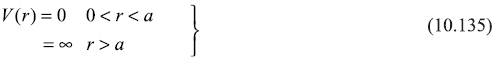
Determine the energy eigenvalue and eigenstate for l = 0 case.
Exercise 10.11
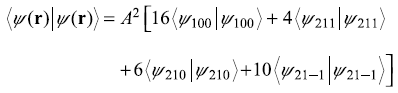
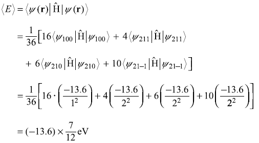
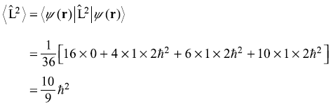
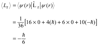
An electron in hydrogen atom is in superposition sate described by the wave function
- What is the value of normalization constant A?
- What is the expectation value of energy E of electron?
- What is the expectation value of
 ?
? - What is the expectation value of
 ?
? - What is ψ(r, t)
Exercise 10.12
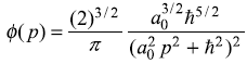
Consider an electron in the ground state of hydrogen atom ![]() . Find out its wave function in momentum space ϕ(p)
. Find out its wave function in momentum space ϕ(p)
Exercise 10.13
Consider a hypothetical case where the electron has equal finite probability of being found anywhere in a sphere of radius R, centred at r = 0, and zero outside it. Find out the radial probability density and show it graphically.
Exercise 10.14
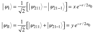
Consider the three ψ2p orbitals, that is ![]() orbitals. One knows that the orbital
orbitals. One knows that the orbital ![]() = (z / a0)e–(r / 2a0) (z = r cosθ) may be written as
= (z / a0)e–(r / 2a0) (z = r cosθ) may be written as ![]() , as it is oriented along z-axis. Write linear combinations of ψ211 and ψ21–1, which are oriented along the coordinate axis x and y.
, as it is oriented along z-axis. Write linear combinations of ψ211 and ψ21–1, which are oriented along the coordinate axis x and y.
Exercise 10.15
While considering sp3 hydridization, one forms four hybrid atomic orbitals (which are orthogonal to each other) as a linear combination of the four-fold degenerate states ![]() . Construct these four hybrid orbitals and show their geometric orientations.
. Construct these four hybrid orbitals and show their geometric orientations.
SOLUTIONS
Solution 10.1
- Normalization of ψ(r, 0) gives
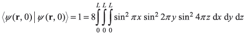
or

∴
L = 1 nm (10.137) - Comparing Eq. (10.131) with the general expression (10.11) of the wave function, we get
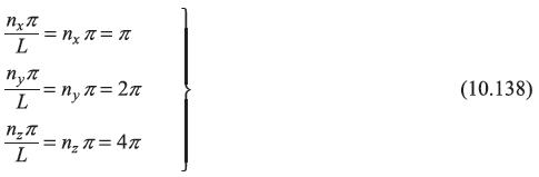
giving
nx = 1, ny = 2, nz = 4 (10.139) - Energy of the electron from Eq. (10.12) is
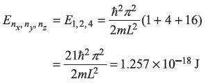
or
E1,2,4 = 7.86eV (10.140) -
ψ124(r, t) = ψ124(r, 0)e–i(E124 / ħ)t (10.141)
- The energy just lower to E1, 2, 4 is the energy of a state corresponding to quantum numbers
nx = 1, ny = 3, nz = 3 (or to nx = 3, ny= 3, nz = 1)
so
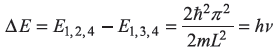
∴

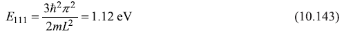
- The ground state corresponds to
nx = ny = nz= 1
Solution 10.2
- Normalization of ψ(r, 0) gives
 ∴ L = 1 nm
 -
Comparing Eq. (10.132) with the general expression (10.20a) of the wave function, we get
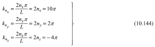
giving
nx = 5, ny = 1, nz = –2 (10.145) - Energy of the electron from Eq. (10.21) is
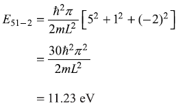
-
E51–2(r, t) = E51–2(r, 0)e–i(E51–2 / ħ)t (10.146)
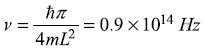
- The energy just lower to E51–2 is the energy corresponding to quantum numbers.
nx = 5, ny= 0, nz = –2 (or any permutation)
(note that in this case, which corresponds to the case of a particle in a box with periodic boundary conditions, ny = 0 is allowed).
so
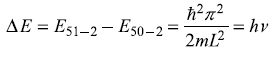
∴
- The ground state corresponds to
nx = ny = nz = 0∴ E0 = 0
Solution 10.3
-
-
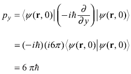
Similarly
pz = 4 πħ -
ψ(r, t) = ψ(r, 0)e–i(77ħπ2 / 2m)t
- The wave function (10.133) represents a wave in the three-dimensional space, whose x-component is stationary wave and y- and z-components are plane propagating waves. A particle confined within two parallel potential walls (in y–z plane) one at x = 0 and the other at x = a (say), shall be described by the wave function (10.133).
- Comparing the given wavefunction with the standard form:
ψ(r, t) = Aei(kx x + ky y + kz z – ωt)
we have
kx = 3ky = 4kz = 5so
Unit vector along the direction of propagation (i.e. along k) is
-
- k = 3ex + 4ey + 5ez
-
-

-
ω = 10π
-

or

or

-
-
E = ħω = 10πħ
Solution 10.5
Wavelength
wave vector
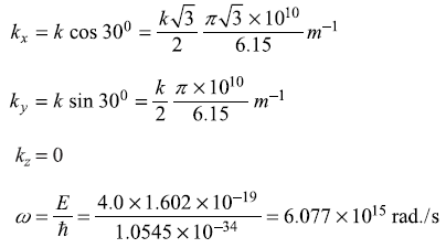
So the wave function is
where kx, ky, ω are given above.
Solution 10.6
- Let there be N free electrons in a one-dimensional solid of length L.
We know from Section (5.5) that the allowed k-values for a free particle in a one-dimensional potential box of length L, within p.b.c., are
The allowed k-values in one-dimensional k-space are shown in Figure 10.6. In ground state at T = 0K, N electrons shall occupy k-states upto Fermi energy EF (or upto Fermi wave vector kF) i.e. all k-states from –kF to +kF are occupied by two electrons (one with spin up and the other with spin down). Therefore
N = 2 × no. of occupied k-states= 2 × 2kF × density of k-points= 2 × 2kF × D(k)or
or
∴

The average energy
 of an electron is given as
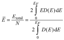
We know for one-dimensional case density of states D(E) is given as [Eq. (10.25)]
so
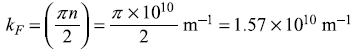
- If we consider N free electrons in a 2-dimensional solid of sides L, the allowed x- and y-components of k-vector are
The allowed k-points are shown in Figure 10.7 in x–y plane. In ground states all k-states within the circle of radius kF are doubly occupied. Therefore
or
∴

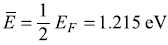
For two-dimensional case density of states D(E) is energy – independent [Eq. (10.28)], so average energy is
Solution 10.7
-
One-dimensional electron gas
-
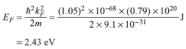
- Two-dimensional electron gas
-
kF = (2nπ)1/2 = (2 × 1019 × 3.14)1/2 m–1= 0.79 × 10¹⁰ m–1
-
-
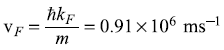
-
-
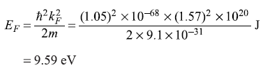
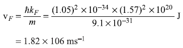
- Three-dimensional electron gas
Solution 10.8
-
Density of states of one-dimensional electron gas is given as
 D(E) at E = E1 = 10–10 eV = 1.6 × 10⁻²⁹ J is
 = 0.507 × 1033 per J= 0.81 × 10¹⁴ per eVD(E) at E = EF = 9.59 eV isD(EF) = 0.26 × 10⁹ per eV
 - For two-dimensional electron gas
 = 1.31 × 1037 per J= 2.10 × 10¹⁸ per eVD(E) at E = EF = 2.43 eV isD(EF) = 2.1 × 10¹⁸ per eV
 - For three-dimensional electron gas
 = 2.24 × 1041 per J = 3.58 × 10²² per eVD(E) at E = EF = 7.85 eV isD(EF) = 10.03 × 1027 per eV
P10(r) is given as
For maxima
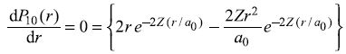
which gives
Solution 10.10
The radial part of the Schrodinger equation for a free particle in the region 0 < r < a, [Eq. (10.59)] is
where ρ = kr

and the radial wave function R(kr) should vanish at r = a, i.e.
Now for l = 0, Eq. (10.59) gives
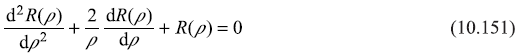
With the substitution u(ρ) = ρR(ρ), above equation gives
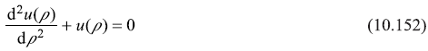
Its solutions are
Therefore the general solution of Eq. (10.151), is
The solution has to be finite at ρ = 0, so the solution remains
Now the condition (10.150) gives
So one gets energy eigenvalues as
and radial part of the wave function as
This is in fact the complete wave function (as for l = 0, Y00 spherical harmonic is angle independent)
Solution 10.11
Solution 10.12
We know from Section 4.10 that the wave function in momentum space is given as
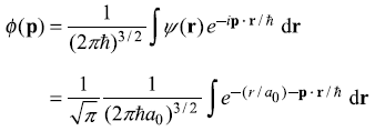
Using the result
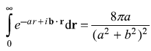
One gets
Solution 10.13
The probability density
As total probability of the electron to be found anywhere within the sphere of radius R is unity,
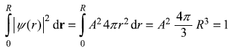
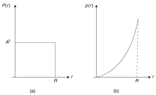
Figure 10.12 (a) Plot of probability density P(r) (b) Plot of radial probability density p(r)
so

Radial probability density p(r) is given as
Plots of probability density P(r) and radial probability density p(r) are shown in Figure 10.12 above.
Solution 10.14
We may have following two combinations giving orthonormal states
We shall denote the states ![]() and
and ![]() as
as ![]() and
and ![]() as these are oriented along x and y-axis respectively.
as these are oriented along x and y-axis respectively.
Solution 10.15
It is easy to construct following four linear combinations (which are orthonormal) out of the four degenerate orbitals ![]()
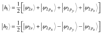
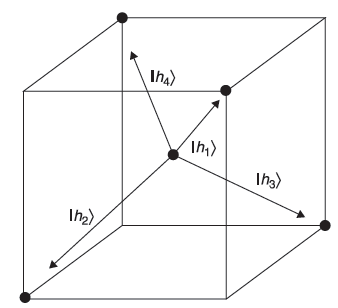
Figure 10.13 A chemical unit cell of the diamond structure. (a chemical unit cell is (1/8)th of the crystal unit cell). One Si atom (an example) is sitting at the centre with four nearest neighbor Si atoms at the four corners. The hybridized orbitals of the silicon atom at the centre have orientations along the directions of the four neighbors
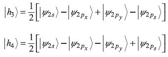
One can easily check that the hybridised wave functions are orthonormal, i.e.,
Figure 10.13 above shows orientations of the four hybrid orbitals ![]() and
and ![]() .
.
REFERENCES
- Ashroft, N.W. and Mermin, N.D. 2001. Solid State Physics. Singapore: Harcourt College Publishers.
- Kinel, C. 2005. Introduction to Solid State Physics. 7th edn., New York: John Wiley and Sons.
- Raimes, S. 1961. Wave Mechanics of Electrons in Metals. Amsterdam: North Holland Publishing Co.
- Condon, E.U. and Shortley, G.H. 1959. The Theory of Atomic Spectra. Cambridge: Cambridge University Press.
- Schiff, L.I. 1968. Quantum Mechanics. 3rd edn., New York: McGraw-Hill.
- Levi, A.F.J. 2003. Applied Quantum Mechanics. Cambridge: Cambridge University Press.
- Bransden, B.H. and Joachain, C.J. 2000. Physics of Atoms and Molecules. 2nd edn., Upper Saddle River, NJ: Prentice Hall.