
chapter 4
BASIC STATISTICAL MEASURES
Objectives:
After completing this chapter, you can understand the following:
Science fiction author H. G. Wells in 1903 stated, “Statistical thinking will one day be as necessary for efficient citizenship as the ability to read and write”. Statistics is a set of perception, procedures and rules that help to organize numerical information in any form such as graphs, tables or charts. It also helps to understand statistical techniques that primarily affect our life in decision making or make informed decisions. Simple statistical tools are available for analytical work like inspection, comparison, quality and precision of the data.
There are descriptive and inferential statistics. To organize or summarize a particular set of measurements, we can use descriptive statistics. That is, a descriptive statistic is described as a set of measurements. For example, a cricket player’s batting average is an example of a descriptive statistic. It describes the cricket player’s past ability to hit a ball at any point in time. This example has a common property that they organize, summarize and describe a set of measurements. To make inferences about the larger population from which the sample was drawn, we can use inferential statistics. For example, we could take the information gained from our service satisfaction from a set of service organizations. Another use of inferential statistics is opinion polls and television rating systems. For example, a limited number of people are polled during an election and then this information is used to describe voters as a whole.
4.1 TYPES OF SCALES
Numbers and set of numbers formulate statistical information specified qualities in the research. The type of statistics used for analysis of data in research is converted into certain types. These types have a great deal of confusion in education and social research that gives in measuring of behaviour. Scale of measure is a classification that describes the nature of information within the numbers assigned to variables. The qualities are magnitude, absolute zero and equal interval. Best statistical procedures can be selected to determine the scale of measurement. The ability to know if one score is greater than, equal to or less than another score is referred as magnitude. The absolute zero referred as a point where none of the scale exists. Here, a score of zero can be assigned. Equal interval is the possible scores that have equal distance from each other. We can determine the four scales of measurement by combining the three-scale qualities. These are nominal, ordinal, interval and ratio scales. Basically, nominal scale is a preparation of a list in an alphabetical order. Alphabetically sorted list of students in a class, list of organizational chart based on hierarchical order and list of favourite actors are the representation of nominal scales. In ordinal data, the magnitude of the data is considered and is looked as any set of data placed in order from the greatest to the lowest without absolute zero and no equal intervals. Likert scale and Thurstone technique are examples of nominal scale types. The interval scale is processed with magnitude and equal intervals without absolute zero. Temperature is an example of interval scale. Since temperature has no absolute zero because it does not exist in the temperature measurement. Ratio scale is the highest scale of measurement. The ratio scale contains three qualities and offers preference to statisticians because ease of analysis. For example age, height and score on a 100-point test are ratio scales. Table 4.1 gives a comparison of each scale.
4.1.1 Nominal Scale
From a statistical point of view, nominal scale is the lowest measurement. It simply places the data into categories without any order or structure. A yes/no is a nominal scale in research activities. For example, in a survey of research answer from the participants can be managed through yes/no scale in order to ease the evaluation. In statistics, the nominal scales are in non-parametric group. Modes and cross tabulation with chi-square are statistical measurement that uses nominal scale.
4.1.2 Ordinal Scale
An ordinal scale is important in terms of power of measurement. For example, consider ranking of beer based on the quality and demand. When a market study for ranking five types of beer from most flavourful to least flavourful is conducted, an ordinal scale of preference can be created. There is no objective distance between any two points on the subjective scale. To one respondent, the brand of the beer may be far superior to the second prefered beer, then another beer is the selection from a respondent. But to another respondant with the same top and second beer, the distance may be subjectively small. An ordinal scale interprets gross order and not the relative positional distances. In statistics, ordinal data would use non-parametric statistics. Median and mode rank order correlation and non-parametric analysis of variance are the statistical techniques.
4.1.3 Interval Scale
One of the standard survey ratings is an interval scale. Suppose the rate of satisfaction of a car service is 10-point scale from dissatisfied to most satisfied by an interval of 1. It is called an interval scale because it is assumed as equidistant points between each of the scale elements; that is, interpretation of differences in the distance along the scale, because we can take the differences in order, not differences in the degree of order. Interval scales are defined by metrics such as logarithms. In logarithms, the distance is not equal but they are strictly definable based on the metric used. Usually in statistics, interval scale data would use parametric statistical techniques such as correlation, regression analysis of variance and factor analysis.
4.1.4 Ratio Scale
It is a top level of measurement and is not frequently on hand in social research. A true zero point is the factor which clearly defines a ratio scale. Measurement of length is the simplest example of the ratio scale. The temperature measurement is the best way to contrast interval and ratio scales. The Centigrade scale has a zero point but it is an arbitrary one. The Fahrenheit scale has its equivalent point at −32°. This way the ratio scale interprets the data.
The fundamental difference between the four scales of measurement is given in Table 4.1.
Table 4.1 Sample database for calculation

4.2 MEASURES OF CENTRAL TENDENCY
A central tendency or measure of central tendency is a typical value for a probability distribution. It is also called centre or location of the distribution. Typically, variability or dispersion is the excellence of the central tendency. Normal distribution set is the key of calculation of the central tendency. Most common measure of central tendency is arithmetic mean and median.
In one-dimensional data, the following techniques may be applied. Before calculating a central tendency to transform the data, the circumstances should be identified.
Mean (arithmetic mean): It is the sum of all measurements divided by the number of observations in the dataset.
Median: It is the middle value that separates the higher half from the lower half of the dataset. The ordinal dataset is used for identification of the median and the mode because values are ranked relative to each other but are not measured absolutely.
Mode: It is the most frequent value in the dataset. In nominal data, this central tendency measure is used because of purely qualitative category assignments.
Geometric mean: For n items in the dataset, it is the nth root of the product of the data values. This measure is valid only for data that are measured absolutely on a strictly positive scale.
Harmonic mean: It is the reciprocal of arithmetic mean of the reciprocals of data values. This measure is valid only for data that are used absolutely on a strictly positive scale.
Weighted mean: It is the arithmetic mean that incorporates weighting to certain data elements.
Truncated mean (or trimmed mean): It is the arithmetic mean of data values after a certain number or proportion of the highest and lowest data values that have been discarded.
Interquartile mean: It is the truncated mean based on data within the interquartile range.
Midrange: It is the arithmetic mean of the maximum and minimum values of a dataset.
Midhinge: It is the arithmetic mean of two quartiles.
Trimean: It is the weighted arithmetic mean of the median and two quartiles.
Winsorized mean: It is the arithmetic mean in which extreme values are replaced by values closer to the median. These techniques are applied to each dimension of multi-dimensional data, but the results may not be invariant to rotations of the multi-dimensional space.
Another set of measurement used in multi-dimensional data are as follows:
Geometric median: It minimizes the sum of distances to the data points. Identification of geometric mean is same as median when applied to one-dimensional data but calculates the median of each dimension independently.
Quadratic mean: It is also known as root mean square, used in engineering, not commonly used in statistics. Major reason of the usage is not a good indicator of the centre of the distribution when the distribution includes negative values.
Parameter: It is a measure concerning a population (e.g., population mean).
4.2.1 Mean, Median and Mode
Simply mean is the average of data, median is the middle value of the ordered data and mode is the value that occurs most often in the data. The measure of central tendency from a population is illustrated in Fig. 4.1.
Due to cost and time factors in most research experimental situations, examination of all members of a population is not typically conducted but examines a random sample, that is, considering representative subset of the population. Parameters are descriptive measures of population. For example, a sample mean is a statistic measure and a population mean is a parameter. The sample mean is usually denoted by x̄ :

Fig. 4.1 Measures of central tendency
where N is the sample size and xi are the measurements.
For example,
Consider the dataset, −1, 1, 2, 3, 13
Here, mean = 4, median = 2, mode = 1
How we arrived at these results?
Steps for finding the median for a set of data:
- Arrange the data in increasing order
- Find the location of median in the ordered data by (n + 1)/2
- The value that represents the location found in Step 2 is the median
For example, consider the aptitude test scores of 10 students,
91, 76, 69, 95, 82, 76, 78, 80, 88, 86
Mean = (91 + 76 + 69 + 95 + 82 + 76 + 78 + 80 + 88 + 86)/10 = 82.1
If the entry 91 is mistakenly recorded as 9, the mean would be 73.9, which is very different from 82.1.
On the other hand, let us see the effect of the mistake on the median value:
The original dataset in increasing order is follows:
69, 76, 76, 78, 80, 82, 86, 88, 91, 95
With n = 10, the median position is found by (10 + 1)/2 = 5.5. Thus, the median is the average of the fifth (80) and sixth (82) ordered value and the median is 81.
The dataset (with 91 coded as 9) in increasing order is as follows:
9, 69, 76, 76, 78, 80, 82, 86, 88, 95
where the median is 79.
Note that the medians of the two sets are different. Therefore, the median is not affected by the extreme value 9.
4.2.2 Geometric and Harmonic Mean
Geometric mean is a particular type of average where we multiply the numbers together and then take the square root (for two numbers), cube root (for three numbers), etc. For example, what is the geometric mean of 2 and 18?
Multiply them: 2 × 18 = 36, the square root: √36 = 6
Geometric mean indicates the central tendency or typical value of a set of numbers by using product of their values. That is, for a set of numbers x1, x2, …, xn, the geometric mean is given as follows:
For example, the geometric mean of the three numbers 4, 1 and 1/32 is the cube root of their product, which is equal to 1/2.
Harmonic mean is a type of average that represents the central tendency of a set of numbers. The harmonic mean of x1, x2, x3, …, xn is

For example, for two numbers 4 and 9 the harmonic mean is 5.54.
4.3 SKEWNESS
It is a measure of degree of asymmetry of distribution. That is, skewness is a measure of symmetry, or more precisely, the lack of symmetry. A distribution of dataset is symmetric if it looks the same to the left and right of the centre point. There are symmetric, left and right skewness. The qualitative interpretation of the skew is complicated. The skewness does not determine the relationship of mean and median. Skewness in a data series may be observed by simple inspection of the values instead of graphical figures. Consider the numeric sequence (99, 100, 101), whose values are evenly distributed around a central value (100). A negative skewed distribution can be obtained by transforming this sequence by adding a value far below the mean. That is, (90, 99, 100, 101). In positive skew, the sequence is by adding a value far above the mean. That is, (99, 100, 101, 110).
- Symmetric: Distribution of mean, median and mode is mound shaped, and no skewness is apparent; such a distribution is described as symmetric (Fig. 4.2).

Fig. 4.2 Symmetric distribution
- Skewed left: In this situation, mean is to the left of the median, long tail on the left (Fig. 4.3). In unimodal distribution, negative skew indicates that the tail on the left side of the probability density function is longer or fatter than the right side. In negative skew, the left tail is longer. That is, the mass of the distribution is concentrated on the right. The distribution is said to be left-skewed, left-tailed or skewed to the left.
- Skewed right: In this situation, mean is to the right of the median, long tail on the right (Fig. 4.4). The positive skew indicates that the tail on the right side is longer or fatter than the left side. In the positive skew, the right tail is longer. That is, mass of the distribution is concentrated on the left. The distribution is said to be right-skewed, right-tailed or skewed to the right.

Fig. 4.4 Right-skewed distribution

4.3.1 Measuring Skewness
For univariate data X1, X2, …, XN, the formula for skewness is:
where x̄ is the mean, S is the standard deviation, and N is the number of data points. This is referred to as the Fisher–Pearson coefficient of skewness.
In normal distribution for any symmetric data, skewness is zero or near to zero. The negative values indicate that data is left-skewed and the positive values indicate that data is right-skewed.
Another formula of skewness is defined by Galton (also known as Bowley’s skewness) is
where Q1 is the lower quartile, Q3 is the upper quartile, and Q2 is the median.
The Pearson 2 skewness coefficient is defined as
4.3.2 Relationship of Mean and Median
The skewness has no strict connection with relationship between mean and median. Negative skew have a mean greater than the median and positive skew in likewise. The mean is equal to the median; if the distribution is symmetric, then the skewness is zero. If the distribution is unimodal, then mean = median = mode. For example, a coin is tossed many times; the series converse is not true in general. That is, zero skewness does not imply that the mean is equal to the median. What happens to the mean and median if we add or multiply each inspection in a dataset by a constant? For example, if a teacher prepares a dataset for an examination by adding five points to each student’s score. What effect does this have on the mean and the median? Altering the mean and median by the constant, the result of adding a constant to each value resulted in an intended effect. Consider that the teacher conducted 10 aptitude scores and the original mean is 82.1 with the median of 81. If 5 is added to each score, the mean of this new dataset would be 87.1 and the new median would be 86. Similarity can be seen by multiplication by a constant; the new mean and median would change by a factor of this constant.
4.3.3 Kurtosis
It is a measure of whether the data are heavy-tailed or light-tailed relative to a normal distribution. The datasets with high kurtosis tend to have heavy tails and the datasets with low kurtosis tend to have light tails. A uniform distribution would be the intense case. Histogram is an effective graphical technique that shows effectiveness of skewness and kurtosis of dataset.
For univariate data X1, X2, …, XN, the formula for kurtosis is given as follows:

where x̄ is the mean, S is the standard deviation, and N is the number of data points.
Selected normal assumptions are made for the classical statistical techniques. Significant skewness and kurtosis clearly indicate that data are not normal.
4.4 MEASURE OF VARIATION
John asked his classmates how many glasses of water they drink on a typical day? From this question, an average measurement or consumption of water for his six friends are marked (Fig. 4.5).
From the analysis of data, one-fourth of the data lie below the Lower Quartile (LQ) and one-fourth of the data lie above the Upper Quartile (UQ). Figure 4.6 gives the placement of data. Measures of variation are used to describe the distribution of the data. The range is the difference between the greatest and the least data values. Quartiles are values that divide the dataset into four equal parts. From these data, questions have been formulated.
- What is the median of the dataset?
- Organize the data into two groups: the top half and the bottom half. How many data values are in each group?
- What is the median of each group?


Fig. 4.6 Data distribution from observation of consuming water
For dataset, measures of average such as mean, mode and median are typical. Within the dataset, the actual values usually differ from one another and from the average value itself. The dataset with high dispersion contains values considerably higher and lower than the mean value. Measures of variation have certain techniques, which describes the distribution of data.
4.4.1 Range
One of the simplest measures of variation is range and calculated by the highest value minus the lowest value.
It is not resistant to change because range only uses the largest and the smallest values and affected by extreme values. In descriptive statistics, the range is the size of the smallest interval which contains all the data that provides a signal of statistical scattering. Representation is most useful in small dataset because it depends on two of the observations.
For example, consider the set A = 4, 6, 9, 3, 7; the lowest value is 3, and the highest value is 9. So the range is 9 − 3 = 6 (Fig. 4.7).

Fig. 4.7 Range
The range can be misleading due to the elements in the set. For example, A = 7, 11, 5, 9, 12, 8, 3600.
Here, the lowest value is 5 and the highest is 3616. Then the range is 3600 − 5 = 3595.
The single value of 3595 makes the range large, but most values are around 10. This can be solved by applying interquartile range or standard deviation.
For example, find the measures of variation for the data (Table 4.2) Range = 70 − 1 or 69 mph Quartile is order the numbers from least to greatest.

Interquartile range is 50 − 8 or 42 UQ − LQ
The range is 69, the median is 27.5, the lower quartile is 8, the upper quartile is 50, and the interquartile range is 42. Median preparation is shown in Fig. 4.8.

Fig. 4.8 Calculation of median
4.4.2 Absolute Deviation
Normal way of calculation of deviation from the mean is to take each score and minus the mean score. For example, the mean score for the group of 100 students we used earlier was 48.75 out of 100. If we take a student who scored 50 out of 100, the deviation of a score from the mean is 50 − 48.75 = 1.25. We can perform same calculation in the dataset to find the total variability of 100 student’s records. This problem may have positive and negative scores, summing up, total deviation becomes zero. How we can analyze the data? By taking the absolute value by avoiding the sign gives absolute deviation. Summing up the total number of scores divided by the total number gives mean absolute deviation. In our example,

where µ is the mean, X is the score, ∑ is the sum of, N is the number of scores, takes the absolute value.
4.4.3 Standard Deviation
Standard deviation is a useful measure of variation. If we observe a small dispersion of a set of data or values are closely bunched about the mean, then standard deviation performs. If a set of numbers x1, x2, x3, …, xn constitute a sample with the mean x̄, then the differences are called the deviation from the mean.
are called the deviation from the mean.
Since all x̄ are not equal, some mean will be negative and some mean will be positive. But Σ(x−(x̄))= 0. the sum of deviations from the mean is Here, the magnitude of mean deviations is considered and simply leave out the signs and define a measure of variation in terms of the absolute values of the deviations from the mean. For n elements in a dataset, we have a statistical measure called mean deviation.
If we work with squares of deviations from mean, the signs are eliminated because square of a real number cannot be negative. So the values after squaring become positive and take the average from the mean and then take the square root of the result. That is,
This is the traditional calculation of the standard deviation. Literally speaking, this is mathematically derived formula, and it is also called root-mean-square deviation. The formula may have some deviations from the mean by n − 1 instead of n. That is, from a sample population, we have sample standard deviation(s)
The population standard deviation is,
where µ is the population mean and N is the number of elements in the population.
What is the purpose of calculating mean, standard deviation and variance? Literally, these statistics estimates corresponding to population parameter give relations between data and dataset. If we draw from many samples from a population that has the mean µ, calculated mean x̄ estimated average of the mean µ, then we can see that the average is close to µ. Even we can calculate the variance of each sample by the formula
Then take the average of estimates and if the average is less then σ2, theoretically we can compensate for this by dividing by n − 1 instead of n in the formula s2.
Example: A biologist found 7, 13, 9, 11, 10, 11, 8 and 7 microorganisms of a certain kind in eight cultures. Calculate S.
Solution: Calculating the mean, we get x̄ = (7 + 13 + 9 + 11 + 10 + 11 + 8 + 7)/8. Now find Σ(x−x̄)2, and it may be arranged as in Table 4.3

By dividing 32.00 by (8 − 1) = 7 and taking the square root, we will get S = 2.14.
In this example, it is very easy to calculate S, because the data are whole numbers and the mean is exact to one decimal. Otherwise, the calculations required by the formula defining S can be quite tedious. We can get S directly with a statistical calculator or a computer by the use of the formula,

4.4.4 Average Deviation
Average deviation or mean absolute deviation of a dataset is the average of the absolute from the central point. First, compute the mean and identify the distance between each score and whether the score is above or below the mean. The average deviation is defined as the mean of these absolute values. The mean absolute deviation of a set x1, x2, …, xn is
The measure of central tendency, m(X), has a marked effect on the value of the mean deviation. For example, for the dataset {2, 2, 3, 4, 14}, see Table 4.4:
Table 4.4 Central tendency and absolute deviation

Mean absolute deviation is calculated by the formula,

4.4.5 Quartile Deviation
Quartile deviation is based on the lower quartile Q1 and the upper quartile Q3. The quartile range is difference Q3 − Q1, which is called the inter quartile range. The difference Q3 − Q1 divided by 2 is called semi-interquartile range or the quartile deviation. That is, QD = (Q3 − Q1)/2.
Comparing range and absolute dispersion, the quartile deviation is a slightly better measure but it ignores the observation on the tails. Values are quite likely to be sufficiently different in the obtained samples from a population by calculation.
Coefficient of quartile deviation
It is a relative measure of dispersion based on the quartile deviation and is given as
It is pure number free of any units of measurement that can be used for comparing the dispersion in two or more than two sets of data.
Example: Calculate the quartile deviation and coefficient of quartile deviation from the data given in Table 4.5.
Table 4.5 Sample database for calculation

Solution: The necessary calculations are given in Table 4.6:
Q1 = Value of (n/4)th item = Value of (60/4)th item = 15th item
Q1 lies in the class 10.25 − 10.75, therefore Q1 = l + h/f(n/4 − c)
where l = 10.25, h = 0.5, f = 12, n/4 = 15 and c = 7, therefore

Q3 lies in the class 11.25 − 11.75, therefore Q3 = l + h/f(3n/4 − c)
where l = 11.25, h = 0.5, f = 14, 3n/4 = 45 and c = 36, therefore
4.4.6 Coefficient Deviation
Coefficient of Variation (CV) or Relative Standard Deviation (RSD) is a standard measure of dispersion of a probability distribution or frequency distribution. Let the standard deviation be σ to the mean µ, then the coefficient of variation is defined as
It shows the extent of variability in relation to the mean of the population.
For example, calculate the coefficient of standard deviation (Fig. 4.9) and the coefficient of variation for the following sample data: 2, 4, 8, 6, 10, and 12.


4.5 PROBABILITY DISTRIBUTION
The outcome of a statistical experiment with its probability of occurrence can be distributed in a table. This is probability distribution that deals variables, random variables and notations. Random variables are subjected to variations by random chances. It is obtained by random experiments such as tossing a coin, rolling a die, selection of card from a pack and picking a number from a given interval. These variables perform unevenness in a function. Probability function is a function that assigns probabilities to the values of a random variable between 0 and 1 inclusive and the sum of the probabilities of the outcomes must be 1. If these conditions are not satisfied by a function, then function is not a probability function. A probability distribution is a function that describes how likely to obtain the different possible values of the random variable.
A discrete variable is obtained from a discrete set of values. Consider rolling of a six- sided die; then the values lie in 1, 2, 3, 4, 5 and 6. For a discrete random variable X and any number x, we can form a probability distribution function P(x). That is, P(x) is the probability that the random variable X equals the given number x which is given by
The random variable must take on some value in the set of possible values with probability 1, so we have P(x) with sum to 1. In equations, the requirements are P(x) ≥ 0 for all x∑x P(x) = 1, where the sum is implicitly over all possible values of X.
For the example of rolling a six-sided die, the probability mass function is
A continuous random variable is a random variable such as a real number or an interval. We cannot make a probability distribution function for a continuous random variable, X by directly assigning a probability. So, a probability distribution function called Probability Density Function (PDF) assigns the probability that X is near each value.
Given the probability density function p(x) for X, we determine the probability that X is in any set A (i.e., X in A) by integrating p(x) over the set A
For a random variable, probability density function with a subscript can be written as
4.5.1 Binomial Distribution
A binomial testing is an experiment that satisfies a fixed number of trials with two outcomes. Each of these trails is independent and probability of each outcome remains constant. Simply binomial tests are experiments with a fixed number of independent trials, each of which can only have two possible outcomes. For example, tossing a coin 20 times to see how many tails occur, asking 200 people if they watch ABC news and rolling a die to see if a 5 appears. The binomial distribution describes the behaviour of a count variable X with the following conditions:
- The number of observations n is fixed.
- Each observation is independent.
- Each observation represents one of two outcomes (“success” or “failure”).
- The probability of success (p) is the same for each outcome.
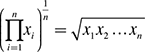
For example, suppose a coin is tossed twice and its outcome is in Table 4.7. These four outcomes are probability of 1/4. Note that the tosses are independent. Hence, the probability of a head on Flip 1 and a head on Flip 2 is the product of P(H) and P(H), which is 1/2 × 1/2 = 1/4. The same calculation applies to the probability of a head on Flip 1 and a tail on Flip 2. Each is 1/2 × 1/2 = 1/4.
Table 4.7 Possible outcomes

Based on the number of occurrence of heads, the four possible outcomes can be classified. The number could be 2 (Outcome 1), 1 (Outcomes 2 and 3) or 0 (Outcome 4). Table 4.7 furnishes the probabilities of these possibilities. Graphically we can represent the probabilities in Fig. 4.10. Since two of the outcomes represent the case in which just one head appears in the two tosses, the probability of this event is equal to 1/4 + 1/4 = 1/2. The situation is summarized in Table 4.8.
Table 4.8 Probabilities of getting 0, 1 or 2 heads

Figure 4.10 shows the probability for each of the values on the x-axis. The head represented as a “success” gives the probability of 0, 1 and 2 successes for two trials. An event has a probability 0.5 of being a success on each trial. This makes Fig. 4.9 an example of a binomial distribution.
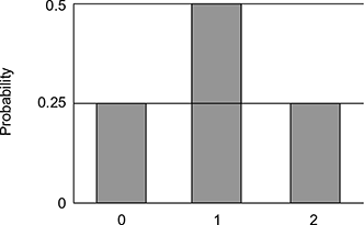
Fig. 4.10 Probabilities of 0, 1 and 2 heads
For N trails, binomial distribution consists of the probabilities for independent events. Each one has a probability of occurring. For the coin tossing example, N = 2 and π = 0.5. Hence, the formula of binomial distribution is
where N is the number of trials, P(x) is the probability of x successes out of N trials, and π is the probability of success on a given trial.
Applying this to the coin tossing example,

Notations
The following notations are helpful while dealing with binomial distribution:
x: The number of successes that result from the binomial experiment.
n: The number of trials in the binomial experiment.
P: The probability of success on an individual trial.
Q: The probability of failure on an individual trial. (This is equal to 1 − P.)
n!: The factorial of n.
b(x; n, P): Binomial probability − the probability that an n-trial binomial experiment results for x successes, when the probability of success on an individual trial is P.
nCr: The number of combinations of n things, taken r at a time.
Example: Suppose a die is tossed 5 times. What is the probability of getting exactly 2 fours?
Solution: In this binomial experiment, the number of trials is equal to 5, the number of successes is equal to 2, and the probability of success on a single trial is 1/6 or 0.167. Therefore, the binomial probability is
4.5.2 Poisson Distribution
Poisson distribution is a discrete probability distribution to model the number of events occurring within a given time interval. The average number of events in the given time interval is represented by λ, which is the shape parameter. Let X is the number of events in a given interval and e is a mathematical constant with e ≈ 2.718282. Poisson probability mass function is
Example: Average rates of 1.8 births per hour in a hospital occur randomly. What is the probability of observing 4 births in a given hour at the hospital?
Solution: X = No. of births in a given hour
Randomly occurred event with a mean rate, λ = 1.8
Using the Poisson distribution formula, calculate the probability of observing exactly 4 births in a given hour.
What about the probability of observing more than or equal to 2 births in a given hour at the hospital?

Figure 4.11 gives the Poisson probability density function for four values of λ.

Fig. 4.11 Poisson probability distribution function for (λ = 5, λ = 15, λ = 25 and λ = 35)
Sum of Two Poisson Variables
Consider the previous example, birth rate in a hospital.
Example: Suppose there are two hospitals A and B. In hospital A, births occur randomly at an average rate of 2.3 births per hour and in hospital B births occur randomly at an average rate of 3.1 births per hour. What is the probability that observed 7 births from both the hospitals in a 1-hour period?
Solution: The following rules have been formed:
If X ∼ Po(λ1) on 1 unit interval and Y ∼ Po(λ2) on 1 unit interval, then X + Y ∼ Po(λ1 + λ2) on 1 unit interval. Let X = No. of births in a given hour at hospital A and Y = No. of births in a given hour at hospital B
Then, X ∼ Po(2.3), Y ∼ Po(3.1) and X + Y ∼ Po(5.4)
4.5.3 Uniform Distribution
A uniform distribution or a rectangular distribution is a distribution with constant probability. The uniform or rectangular distribution has random variable X restricted to a finite interval [a, b] and has f(x) has constant density over the interval. An illustration is given in Fig. 4.12. There are discrete and continuous uniform distributions. The outcome of throwing a fair dice is a simple example of the discrete uniform distribution. The probability of each outcome is 1/6 from the possible values 1, 2, 3, 4, 5 and 6. While adding each probability resulting distribution is no longer uniform since not all sums have equal probability.
Fig. 4.12 Rectangular distribution
The function F(x) is defined by

The expectation and variance are given by the formulae

Example: The electric current (in mA) measured in a piece of copper wire is known as uniform distribution over the interval [0, 25]. Write down the formula for the probability density function P(x) of the random variable X representing the current. Calculate the mean and variance of the distribution and find the cumulative distribution function F(x).
Solution: Over the interval [0, 25], the probability density function f(x) is given by the formula

Using the formulae developed for the mean and variance gives

The cumulative distribution function is obtained by integrating the probability density function by
![]()
Hence, choosing the three distinct regions, x < 0, 0 ≤ x ≤ 25 and x ≥ 25, gives

4.5.4 Exponential Distribution
The exponential distribution is the probability distribution that describes the time between events in a Poisson process. Figure 4.13 illustrates the different exponential distribution. It gives plot of the exponential probability density function and exponential cumulative distribution function. That is a process in which events occur continuously and separately at a constant average rate. The equation for the standard exponential distribution is f(x) = e x for x ≥ 0.

Fig. 4.13 Exponential distribution
The formula for the cumulative distribution function of the exponential distribution is
Example: The number of kilometres that a particular car can run before its battery wears out is exponentially distributed with an average of 15,000 km. The owner of the car needs to take a 7500-km trip. What is the probability that he will be able to complete the trip without having to replace the car battery?
Solution: Let X denotes the number of kilometres that the car can run before its battery wears out. Consider that the following is true:
It is noticed that the probability that the car battery wears out in more than y = 7,500 km does not subject if the car battery was already running for x = 0 km or x = 1,500 km or x = 22,500 km. Given that X is exponentially distributed because of the above true statement for the exponential distribution.
That is, if X is exponentially distributed with mean θ, then
Therefore, the probability in question is simply
From this, we can decide that the probability is large enough to give him comfort that he won’t be stranded somewhere along a remote desert highway.
4.5.5 Normal Distribution
The normal distribution or Gaussian distribution is a very common continuous probability distribution. This is highly applicable in social and natural science.
A normal distribution formula is
where µ is the mean and σ2 is the variance.
Empirical rule
For bell-shaped distributions, about 68% of the data will be within one standard deviation of the mean, about 95% will be within two standard deviations of the mean, and about 99.7% will be within three standard deviations of the mean (Fig. 4.14)
Example: An IT company that has employees hired during the last 5 years is normally distributed. Within this curve, 95.4% of the ages, centred about the mean, are between 24.6 and 37.4 years. Find the mean age and the standard deviation of the data.
Solution: The mean age is symmetrically located between −2 standard deviations (24.6) and + 2 standard deviations (37.4).
The mean age is 31 years of age.
From 31 to 37.4, (a distance of 6.4 years) is 2 standard deviations. Therefore, 1 standard deviation is (6.4)/2 = 3.2 years.

EXERCISES
- What is the best measure of central tendency?
- In a strongly skewed distribution, what is the best indicator of central tendency?
- Does all data have a median, mode and mean?
- When is the mean the best measure of central tendency?
- When is the mode the best measure of central tendency?
- When is the median the best measure of central tendency?
- What is the most appropriate measure of central tendency when the data have outliers?
- In a normally distributed dataset, which is greatest: mode, median or mean?
- For any dataset, which measures of central tendency have only one value?
- Table 4.9 shows a set of scores on science test in two different classrooms. Compare and contrast their measures of variation.
Table 4.9 Database

- The normal monthly rainfalls in inches for a city are given in Table 4.10. What are outlier values of the following table?
Table 4.10

- Suppose a die is tossed. What is the probability that the die will land on 5?
- Data on the number of minutes that a particular train service was late have been summarised in Table 4.11
(Times are given to the nearest minute.)
Table 4.11 Database

- How many journeys have been included?
- What is the modal group?
- Estimate the mean number of minutes the train is late for these journeys.
- Which of the two averages, mode and mean, would the train company like to use in advertising its service? Why does this give a false impression of the likelihood of being late?
- Estimate the probability of a train being more than 20 minutes late on this service.
- What is the Geometric Mean of 10, 51.2 and 8?
- The amount of time that John plays video games in any given week is normally distributed. If John plays video games an average of 15 hours per week, with a standard deviation of 3 hours, what is the probability of John playing video games between 15 and 18 hours a week?