
chapter 5
DATA ANALYSIS
Objectives:
After completing this chapter, you can understand the following:
- The definition of statistical analysis and its types
- The description of multivariate analysis
- The definition of correlation analysis and its limitations
- The definition of regression analysis and its case study
- The detailed explanation of principle component analysis
- The definition of sampling and its various types
- The description of SPSS (a statistical analysis tool) and its file types and analysis functions
What is the human development index (HDI) value of India in 2013? Who is analyzing HDI? What is the scale rating of HDI? Is there any role for stock market in the development of HDI? What is the health rate score in India?
These questions have common elements. The answers may have some data part that helps in determining facts. Data analysis is a method or procedure that helps to describe facts, detect patterns, provide explanations and test hypothesis. It is highly used in scientific research, business and policy administration.
The output of data analysis may be numeric results, graphs, etc. For numerical results, values such as average income of a group or temperature difference from year to year, etc. may be taken into consideration. For example, between 2001 and 2011, the population of India has increased by 181 million people, out of which 91 million are males and 90 million are females. This is a fact and can interpret that there is a growth of 18 million people per year. From these, can we conclude that, after 30 years a growth of 543 million people from the present population status will occur? This interpretation may be wrong. The Indian population cannot be predicted in such an approximate way.
Different data analysis techniques are given in Fig. 5.1. The techniques include statistical analysis, multivariate analysis (MVA), regression analysis, etc. Using these analyses, a researcher finds facts, relations and outputs from the collected data.

5.1 STATISTICAL ANALYSIS
How will we collect, explore and present large amount of data? To discover patterns and trends in a large amount of data, we can use the statistical data analysis. In our day-to-day life, statistics plays a significant role in decision making. The use of statistics helped to research, industry, business and government to make important decisions.
Statistical analysis is a component of data analytics that involves collecting and scrutinizing every data sample in a set of items from which samples can be drawn. Trends identification is one of the goals of statistical analysis, which identify patterns in unstructured and semi-structured data for business analysis. In statistical analysis, two important terms are required to notice – population and sampling. Population is a total inclusion of all people or items with similar characteristics or wishes. Sampling is central to the discipline of statistics. From the population, samples are made in order to obtain selected observations. This is a feasible approach that saves cost and time because sampling gives a snapshot of a particular moment. When the population is uniform, a perfect representation is possible in the sampling. Sampling errors occur when a difference in the measured value for an attribute in a sample from the “true value” in the population. A detailed explanation of population and sampling is given in Section 5.6.
Figure 5.2 gives steps involved in statistical analysis. Hypothesis testing plays major role in the statistical analysis. Chapter 6 gives detailed account of statistical test procedures.
Qualitative and quantitative data are two types of data in statistical analysis. Qualitative data is a categorical measurement expressed not in terms of numbers, but described by means of a natural language. For example, “height = tall”, “colour = white”. Quantitative data is a numerical measurement expressed in terms of number, not in natural language. For example, “length = 450 m”, “height = 1.8 m”.
Inferential statistics and descriptive statistics are two types of statistical analysis. Inferential statistics (confirmatory data analysis) used information from a sample to draw conclusions about the population from which it was drawn. Descriptive statistics (exploratory data analysis) investigates the measurements of the variables in a dataset. In descriptive statistics, the attributes of a set of measurements are characterized. To explore patterns of variation, and describe changes over time, summarized data are used. The inferential statistics are designed to allow inference from a statistic measure on sample of cases to a population parameter. A hypothesis test to the population is used in data analysis. Figure 5.3 shows different types of statistical methods.


Fig. 5.3 Types of statistical methods
Different types of descriptive and inferential statistical methods are given in Figs. 5.4 and 5.5, respectively.

Fig. 5.4 Types of descriptive methods

The details of these methods are given in Chapter 7. The examples of some commonly used statistical tests are given in Fig. 5.6. These tests are based on level of measurements. Most of the tests are covered in this book.

Fig. 5.6 Examples of some commonly used statistical tests
5.2 MULTIVARIATE ANALYSIS
How can we analyze two sets of data in a simultaneous statistical process? When more than two variables involved, how statistical analysis is being done? A MVA technique is a statistical process that allows more than two variables to be analyzed at once. Otherwise, we can define as multivariate data analysis is a statistical technique used to analyze data that arises from more than one variable. There are basically two general types of MVA technique – analysis of dependence and analysis of interdependence. With respect to analysis of dependence, one or more variables are dependent to be explained or predicted by others. Multiple regression, Partial Least Squares (PLS) regression and Multiple Discriminant Analysis (MDA) are various methods of dependence MVA. In analysis of interdependence, we will not choose any variables that are thought of as “dependent” and look at the relationships among variables, objects or cases. Cluster analysis and factor analysis are certain interdependence MVA techniques. The MVA technique is useful where each situation, product or decision involves more than a single variable.
The MVA is used in the following areas:
- Market and consumer research
- Across a range of industries, quality control and quality assurance. The industries such as food and beverage, pharmaceuticals, telecommunications, paint, chemicals, energy and so on are used MVA technique for information formulation.
- Process control and optimization
- Research and development
The MVA technique depends upon the question: Are some variables dependent upon others? We can use dependence methods, if the answer is “yes”. Otherwise, we can use interdependence methods. To select a classification technology, two more questions are required to understand the nature of multivariate techniques. First, if the variables are dependent, how many variables are dependent? Another question is, whether the data are metric or non-metric? This is about collected quantitative data on an interval or ratio scale. We can say whether the data are qualitative, collected on nominal or ordinal scale. Figure 5.7 gives the flow chart that explains how to arrive multivariate techniques from a variable. Various MVA techniques are given in the following.
Factor analysis
Consider a research design with many variables, which reduces the variables to a smaller set of factors. There is no dependent variable used in this technique. A researcher looked into the underlying structure of the data matrix, for a sample size. Normally, the independent variables are normal and continuous. Common factor analysis and principle component analysis are two major factor analysis methods. The first one is used to look into underlying factors, while the second one is used to find the fewest number of variables that explain the variance.
Cluster analysis
To reduce a large dataset to meaningful subgroups of individuals or objects, we can use cluster analysis. Based on similarity of the objects across a set of specified characteristics, the division is made. The correlation of the data in the population gives clusters. Hierarchical and non-hierarchical clustering are two clustering techniques used in data analysis. For smaller datasets, hierarchical technique is used. The non-hierarchical technique is used in larger dataset with priorities.
Multiple regression analysis
Relationship between a single metric dependent variable and two or more metric independent variables is examined by this technique. This technique determines linear relationship with the lowest sum of squared variances. The assumptions are carefully observed. Weights are the minor impacts of each variable and the size of the weight can be interpreted directly.
Logistic regression analysis
It is a choice model that allows in prediction of an event. The objective is to arrive at a probabilistic assessment of a binary choice. The variable chosen is either discrete or continuous. An event match is seen in the classification of observations for observed and predicted events. These matches are plotted into a table and used in data analytics.

Discriminant analysis
For correct classification of observations or people into homogeneous groups, we can use this technique. The independent variables have a high degree of normality and are seen as metric. To classify the observations, the discriminant analysis builds a linear discriminant function. A partial value is calculated to determine variables that have the most impact on the discriminant function. The higher the partial value, the more impact the variable has on the discriminant function.
Multivariate Analysis of Variance (MANOVA)
To examine the relationship between two or more metric dependent variables and several categorical independent variables, we can use MANOVA. Across a set of groups, this technique examines the dependence relationship between a set of dependent measures. The MANOVA analysis is useful in experimental design. MANOVA uses the hypothesis tests in problem domains which can be practically solved.
Multi-dimensional Scaling (MDS)
It is useful in visualizing the level of similarity of individual cases of a dataset. An MDS algorithm identifies between-object-distances that are preserved as well as possible. Each object is then assigned coordinates in each of the N dimensions.
Correspondence analysis
This technique provides a dimensional reduction of objects by examining the independent variables and dependent variables at the same time. When we have many companies and attributes, this technique is useful.
Conjoint analysis
It is a trade-off analysis method used in market research to determine how people value different attributes. It is a particular application of regression analysis. The objective of conjoint analysis is to determine what combination of a limited number of attributes is most influential on respondent choice. A controlled set of potential products or services is shown to respondents, and by analyzing how they make preferences between these products, the implicit valuation of the individual elements making up the product is determined.
Figure 5.8 shows the various attributes and levels of attributes in a typical conjoint analysis technique. The figure explains the various variables that a customer typically uses while buying a television.
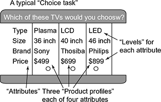
Fig. 5.8 Conjoint analysis
The various steps in conjoint analysis are as follows:
- Choose product attribute
- Choose values for each attribute
- Define products as a combination of attribute options
- A value of relative utility is assigned to each level of an attribute called part-worth utility
- The combination with the highest utilities should be the one that is most preferred.
There are basically two methods by which conjoint analysis can be done: one is Paired comparison and the other one is Full profile comparison. In paired, just two attributes/features will be selected while multiple attributes are selected in full profiling. Paired makes the respondents easy to comment on, but it can be sometimes unrealistic inputs.
Limitation to conjoint analysis
- Assumes that important attributes can be identified
- Assumes that consumers evaluate choice alternatives based on these attributes
- Assumes that consumers make trade-offs (compensatory model)
- Trade-off model may not represent choice process (non-compensatory models)
- Data collection can be difficult and complex
Canonical correlation
Suppose there are two vectors X = (X1, …, Xn) and Y = (Y1, …, Ym) of random variables, and there exists a correlation among these variables. Canonical-correlation analysis is used to find linear combinations of Xi and Yj which have maximum correlation with each other. A typical use for canonical correlation in the experimental context is to take two sets of variables and see what is common amongst the two sets.
Structural Equation Modelling (SEM)
To identify multiple relationships between sets of variables simultaneously, we can use SEM. For example, human intelligence cannot be measured directly by a measure of height or weight. A psychologist develops theories to measure intelligence by executing the use of variables. The SEM technique is used to test with data gathered from people who took their intelligence test.
5.3 CORRELATION ANALYSIS
Correlation and regression analysis are related measures because both of them deal with relationship of variables. Correlation is a measure of linear association between two variables. The correlation value is always between −1 and +1. If two variables are perfectly related in a positive linear sense, then the correlation co-efficient is +1. Similarly when correlation co-efficient is −1, it indicates two variables which are perfectly related in a negative linear sense. If there is no relation between two variables, then the correlation co-efficient is 0.
Suppose a random variable X is distributed with a series of n measurement and Y = X2. Here, Y is perfectly depended on X. The two variables X and Y are written as Xi and Yi where i = 1, 2, …, n.
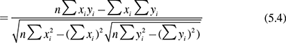
Sample correlation co-efficient can be estimated as Pearson correlation R between X and Y as shown in Eqs. 5.1 and 5.2:


where x̄ and ȳ are sample means of X and Y, respectively. Sx and Sy are sample standard deviations of X and Y. Equations 5.3 and 5.4 summarize this process

The correlation co-efficient is between −1 and +1. The degree of correlation is shown in Fig. 5.9. Strong positives and strong negatives tend to +1 and −1, respectively. When weak positives or weak negatives occur, the points plotted are scattered across. A pure scatter diagram is obtained for a zero correlation.
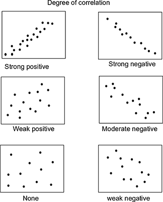
Fig. 5.9 Degree of correlation
In positive correlation, high values of X are associated with high values of Y and in negative correlation high values are associated with low values of Y. For a null correlation, the values of X cannot predict the values of Y. That is, they are independent of each other. Figure 5.10 shows positive, negative and null correlation.
When all points fall directly on a downward line, then r = −1. Similarly, when the scatter plot falls directly on an upward line slope, then r = ±1. These are called perfectly negative and perfectly positive correlation (Fig. 5.11).
Strong correlations are associated closely to the imaginary tied line. When value of r is closer to +1, stronger positive correlation occurs and when it is closer to −1 stronger negative correlation happens. Figure 5.12 shows the stronger and weaker correlation subjective to certain points plotted. However, visually correlation strength can never be qualified as it is a subjective measurement.


Fig. 5.11 Perfect correlation
Based on the Pearson correlation co-efficient, we can identify correlation strength by the value of r.
0.0 ≤ |r| ≤ 0.3 Weak correlation
0.3 ≤ |r| ≤ 0.7 Medium correlation
0.7 ≤ |r| ≤ 1.0 Strong correlation
For example, +0.881 is a strong positive correlation.

The one discussed here is the Pearson correlation co-efficient. Do you know any other correlation co-efficient? Another such correlation co-efficient is Spearman’s rank correlation co-efficient. This correlation co-efficient is used in a population parameter and as rs for sample statistic. This is used when one or both variables are skewed, when extreme values are there. Consider X and Y as variables and the formula for Spearman’s correlation co-efficient is shown in Eq. 5.5. rs shows the difference in ranks for X and Y.

Difference between correlation and regression
We can understand that correlation and regression are two measures of dependency of variables. How can we discriminate one from the other? In order to understand the difference, take an example of two variables, crop yield and rain. These variables can be measured at different places and scale. One is used in farmer’s scale and the other is at weather forecasting station. Correlation analysis shows a high degree of association between these two variables. The regression analysis shows the dependence of crop yield on rain. But careless data collection demonstrates that rain is dependent on crop yield. This type of analysis concludes that in a heavy rainy season there is guaranteed big crop yield. This may be an error conclusion.
Limitations of correlation
One major disadvantage of correlation co-efficient is that it is computationally intensive. The correlation co-efficient is sensitive to imaging systems. It measures linear relationship between X and Y; therefore, change in X will proportionally change Y. If the relationship is non-linear, the result is inaccurate. It is meaningless for categorical data such as colour or gender.
5.4 REGRESSION ANALYSIS
Regression is one of the powerful statistical analysis techniques used to predict continuous dependent variable from a number of independent variables. Or in other words, regression is a technique to determine linear relationship between two or more variables. Primary use of regression technique is prediction analysis of naturally occurring variables to extremely manipulated variables. A natural terminology is used for predicting Y from the known variable, X. The variables used in regression analysis can be either continuous or discrete. The simplest form of regression shows a relationship between the above said variables X and Y formulated as
where i = 1, 2, … n, Ui is the random error associated with an ith observation, W0 is the intercept parameter and W1 is the slope parameter. The slope parameter gives magnitude and direction of the relation. Linear regression computes W1 from a dataset to minimize the error to fit the data (Fig. 5.13).

Fig. 5.13 Linear regression
For example, let “income” and “educational level” be two dataset whose relationship needs to be analyzed. This will create a normal distribution of independent volumes. Consider another example, in which a researcher has a set of collected data on home sales prices and the actual sales prices. Table 5.1 furnishes the data from a collected resource useful in regression analysis.
Table 5.1 Home sales
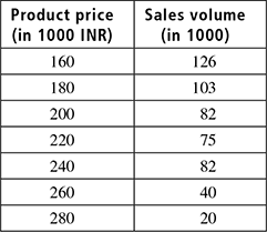
The data are collected for a month from a particular geographical area. We want to know the relationship between X and Y. Figure 5.14 shows the relationship plotted in a graph by using the formula
where Y is the observed random variable (response variable), X is the observed non-random variable (prediction value), W0 is the population parameter – intercept, W1 is the population parameter – slope co-efficient, U is the unobserved random variable.

Fig. 5.14 Graph plotted
Here no straight line can be exactly plotted through the points. In each observation, the line that fits “best” is one of the vertical distance measures. This is called residual error. How will you calculate W0 and W1 here? The answer is by Ordinary Least Squares (OLS) regression procedure. Using OLS, one can calculate the values of W0 and W1 (intercept and slope) that shows best fit observation. In order to calculate OLS, certain assumptions are made in a linear regression technique as mentioned in the following:
- Selected linear model is correct.
- Non-liner effects are omitted (e.g., area of circle = πr2, r is the radius).
- The mean of unobservable variable not depends on observed variable.
- No independent variable predicts another one exactly.
- In repeated sampling, independent variables are fixed or random.
By unvarying these assumptions, we need to identify a best fit associated with n points. In the two-dimensional space points (x1, y1), (x2, y2), …, (xn, ym) has the form
In our example (home sales collected data, Table 5.2), the values of slope and intercept are as follows:
Table 5.2 Home sales


Now y = mx + b, becomes
and it is our least square line.
Conclusion
For every one unit increase in the price of house hold items, 0.7929 fewer house hold items are sold. This is our co-efficient. If the regression were performed repeatedly with the same variable on a different dataset, there may be a standard error in the estimated co-efficient. In this regression analysis, we have to consider only W1 and U due to its linearity. Figure 5.15 shows how the curve is exactly fitted with respect to the points by its slope and interception.
Case Study
The human Body Mass Index (BMI) is calculated by ratio of weight (kg) and square of height (m2).
A data collection contains 10 people’s height and weight in the tabular form. Can you plot these values on a graph with weight on x-axis and height on y-axis? How will you calculate the linear relationship between the height and the weight? How will you fit a straight line linearly in the graph? Figure 5.16 shows the points plotted on the graph. You should cluster points and find a slope upwards on the graph. Then find out taller people with more weight. The regression analysis may have an equation of a line that fits in the identified cluster of points with minimum deviation. This deviation is called error. In your regression equation, if a person’s weight is known, then the height can be predicted.


Fig. 5.16 BMI plot
Let us take the case of a researcher who likes to study the elephant’s details from its foot prints. Samples of leg lengths and skull size from a population of elephants are collected. The two variables selected in the study are “leg length” and “skull size” that are associated in some way. The elephants with short legs may have big heads. So, an association may be found in these variables. Regression is an appropriate bag to describe a relationship between head size and leg length. Is it correct? If the skull size increases, the length of leg increases? Does size is a cause for small skull? The answers to these questions can be concluded by the regression analysis of two variables.
Failures of linear regression
Linear regression may fail when false assumptions are made. For example, when you consider more independent variables than the observations, false assumptions are made. Another failure of linear equation is it only looks a linear relationships between dependent and independent variables. That is, when a straight line relationship is between two variables (e.g., income and age), there may be a curve that can be fitted and is incorrect because of the income.
5.5 PRINCIPLE COMPONENT ANALYSIS
Principle Component Analysis (PCA) is a widely used mathematical procedure in exploratory data analysis, signal processing, etc. It was introduced by Pearson (1901) and Hotelling (1933) to describe the variation in a set of multivariate data in terms of uncorrelated variable sets. It is widely used as a mathematical tool for high dimensional data analysis. However, it is often considered as a black box operation whose results and procedures are difficult to understand. PCA has been used for face recognition, motion analysis, clustering, dimension reduction, etc. It provides a guideline for how to reduce a complex dataset to a lower dimensional one to reveal the underlying hidden and simplified structures. There are a lot of mathematical proofs and theories involved in PCA, but here we are not discussing them, we are just outlining how the analysis is carried out.
The following are the various steps involved in PCA:
- Get the data
The aim of our study is to analyze the data; so the primary requirement is to get the dataset. We have already mentioned the various methods of data collection schemes. Any of those approaches may be used for collecting the data. In case of result comparisons, already processed datasets will be available in the logs and data bank. Anyhow, acquiring the dataset is the primary step in PCA.
- Data adjustment
For the analysis to carry out smoothly, the data need to be polished. For this process, you have to subtract the mean from each data dimension. That is, all x values will have x̄ subtracted and all y value will have ȳ subtracted from it respectively (if the selected data is a 2D dataset). This produce a dataset with zero mean.
- Covariance matrix is calculated
Covariance is usually measured between two dimensions. But whenever we have more dimensions, more covariant values need to be calculated. In general, for n-dimensional dataset, we need to calculate play style
 . When we are having more dimensions, what we do is, calculate the covariance between two different dimensions. For example, in an “n” dimension matrix, the entry on row 2, column 3 is the covariance value calculated between the second and third dimensions.
 - Calculate the eigen vectors and eigen values of the covariance matrix
To do this, we find the values of λ which satisfy the characteristic equation of the particular matrix. If A is the matrix, we find A − λI, then find the determinant of (A − λI). Now solve the equation we obtained and the result gives you the eigen values. Once the eigen values of a matrix (A) have been found, just find the eigen vectors by Gaussian elimination.
- Project and derive the new dataset
Once we have chosen the components (eigen vectors) that need to be incorporated in our data, we find the new feature by taking the transpose of the vector and multiply it on the left of the original dataset. That is,
Final Data = Row Feature Vector × Row data Adjust.Principle component analysis accounts for the total variance of the observed variables. If you want to see the arrangement of points across many correlated variables, you can use PCA to show the most prominent directions of the high-dimensional data. Using PCA, the dimensionality of a set of data can be reduced. Principle component representation is important in visualizing multivariate data by reducing it to two dimensions. Principle component is a way to picture the structure of the data as completely as possible by using as few variables as possible.
5.6 SAMPLING
Suppose we need to collect the names of all developed countries in the world. How we are going to do this? What are the criteria for this selection?
How will you collect a group of zoology scholars from a large scholar’s group? These are the generation of subset from a larger set. So, sampling is a technique of subset creation from a population. A population can be defined as total inclusion of all people or items with similar characteristics or wishes. Researchers who are interested in the study of a selected population group are called target population. Researchers make conclusions from the target population. For example, in a social research conducted for the survey regarding heart attack of men aged between 35 and 40 years. The purpose of this study is to compare the effectiveness of certain drugs in order to delay or prevent the future heart attacks. All men who meet some general criteria are selected in the target group and is included in the actual study.
Samples are subset of population (Fig. 5.17a) obtained by subgroups (Fig. 5.17b). Sample selection is important when it comes to reality. Suppose our population is unmanageably large (geographically scattered), studies on this group may be considerably expensive and consume more effort. So, sample selection is important too when the population size increases. Sampling steps include population identification, sample size identification and sample selection.
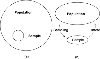
Fig. 5.17 Population and sample
5.6.1 Important Terms
Universe: The entire items or units in any study of enquiry.
Population: Information-oriented items that possess some information or common characteristics. This may be real or hypothetical.
Elementary units: A selected unit that possess relevant characteristics of a population. These constitute the attributes in the object of study.
Sampling frame: Frame is constructed by a researcher or using some existing common population used in the study. This frame must satisfy completeness, accurateness, adequateness and should be up to date.
Sample design: The target population selection needs a plan from a sampling frame. There are many techniques that provide good sample design.
Parameters: Certain characteristics of a population.
Statistics: Characteristics of a sampling frame with specific objectives achieved by analysis.
Sampling errors: Errors that occur at the time of sampling. The errors can be measured as
Precision and accuracy: Precision and accuracy are measurements of a system in the degree of closeness.
Confidence level: Expected percentage of times that actual result falls in the fixed precision range.
Significance level: Predicted results fall outside the range.
5.6.2 Characteristics of Good Sample Design
In order to select good samples from a population, there are certain characteristics.
A representative sample: Suppose a researcher selects a small number of closely matched samples from a population, it will help to generalize the results for a large universe being studied.
Sampling error should be minimized: Sampling error is caused in small samples obtained from a population. It is a discrepancy in the original and obtained values. Efficient design and estimation strategies will reduce such errors.
Economically viable: If the sample collection is expensive, it will not fit to the research budget. Ensure that the sampling must be within the budget and reduce its expenses.
Marginal systematic bias: A systematic approach gives less error in the sampling procedure that will not reduce the sample size.
Generalized samples: Population may be larger and geographically distributed. When sample creation for the research is carried out, it must be generalized; then the errors will come down and the sample covers the whole universe.
Applicable to population: When we select a sample, it should be noticed that it covers the entire population of the study. The sample selection should not be limited to a part so that the entire population is satisfied.
5.6.3 Types of Sampling
Basically, there are two sampling techniques, probability sampling and non-probability sampling (Fig. 5.18).

Fig. 5.18 Types of sampling
Probability sampling
In this type of sampling, the samples are based on probability theory. A non-zero chance of selection is made in every sample unit.
- Simple random sampling
This is one of the most widely known types of sampling characterized by same probability selection for every sample in the population. Simple random sampling selects n items from a population of size N such that every possible sample size has an equal chance. For example, if we want to conduct a survey regarding the next municipal election, we have to select 1,000 voters in a small town with population of 1,00,000 eligible voters. The survey is conducted with the help of paper slips. There are 1,000 slip samples selected by random locations in the town. We have a random selection procedure for each people in the location of the town.
Case Study
Suppose a social researcher wants to conduct a survey in a medium town of population 1.5 million people regarding the waste management and disposal system of the municipal corporation. For this, the researcher should collect the telephone numbers from the directory that contains 3 lakh entries. Then the researcher may select 1,000 numbers in various locations using random sampling technique. He/She may start between 1 and N/n and take every 300th name.
- 2. Stratified random sampling
As we have seen that in sampling the entire population is divided into two or more mutually exclusive segments based on research interest. In the population, data may be scattered so that homogeneous subsets are required before sampling. Each subunit in the subgroup is called “strata”. The researcher systematically divides the groups into subgroups based on his/her interest. For example, an institute in South India needs to take sample students who are from south region of the country as well as foreign origin. The population contains 10,000 students and its strata contain 6,000 – Tamil Nadu, 2,000 – Kerala, 1,000 – Karnataka, 500 – other regions and 500 – foreign students. Suppose the researcher is interested in the sample from Kerala students, then ensure that for further study percentage of students in each group must be selected by random sampling method. This is nearly same as stratified random sampling. Stratification sampling is a popular technique and can be chosen for wide applications, because
- Sampling is done independently in each status so that each subgroup has precision.
- Management by stratification from a large population is conveniently high. Example: Branch Officers conduct surveys from the main population.
- Sampling is inherent in certain subpopulation. Example: Students in a college living in hostels.
- Characteristics of the entire population may improve by stratification.
- Division of homogeneous and heterogeneous subpopulation is possible.
- Statistical advantage in the method with small variance with parameters of interest.
- 3. Systematic random sampling
This sampling method is same as simple random sampling but subgroups are not selected randomly. For example, you have a population with 10,000 records and you want a sample of 1,000. We can create systematic random samples by
- Number of cases in the population is divided by the number of required size. In the above example, it is 10,000/1,000 gives a value 10.
- Value has been selected between 1 and the attained value in the previous step of the above example: the value should be between 1 and 10 (e.g., 5)
- A step factor should be added to the selected value for the successive records. In the above example, we are selecting the record numbers 6, 15, 25, …
There are many advantages of systematic sampling over simple random sampling. One of them is lesser mistakes while sample designing. We can expect precise samples within one stratum. Bias sources can be eliminated by this sampling technique.
- 4. Cluster sampling
Cluster is a group of item with similar nature. In certain instance, the sampling units need to be grouped into smaller units. For example, general election opinion in South India, North India, Southwest India, etc. is collected for total election results. The states can be grouped together or clustered at the time of sampling. When cluster sampling is chosen, certain points should be noted.
- Clustering is done in large scale surveys.
- The other type of random sampling can be combined with random sampling (clustering with strata).
- Generally, for a given sample size and cluster, clustering sampling is less accurate than the other type of sampling.
In cluster sampling, all items are included in the study; each of them may be focussed in any of the groups or clusters. Figure 5.19 shows cluster sampling.

Fig. 5.19 Cluster sampling
Case Study
Suppose the agriculture department, Government of India, wishes to investigate the use of pesticides by the farmers in India. Different states in India can form clusters. For example, South Indian States (Kerala, Tamil Nadu, Karnataka and Andhra Pradesh) produce more rice than other clusters like Central India (Cluster contains Madhya Pradesh, Chhattisgarh, Maharashtra). A sample of other clusters (states) would be chosen at random so that farmers are included in the sample. It is easy to visit several farmers (even they are different in crop plantation) to understand the use of pesticides. The group who visited may have good idea about what the farmers produced with their interest.
Non-probability Sampling
Large-scale surveys are conducted in social researches. For example, say we want to study problems related to homeless people. Here, the information gathering is a tedious task. In such cases, non-probability methods are adapted for the sampling purpose. Primary difference between probabilistic and non-probability methods of sampling is the element of population selected for the study. Four major non-probability sampling methods are discussed here.
- Availability sampling
Availability sampling is otherwise stated as convenience sampling. The researcher selects units that are accidental or close at hand. Primary advantage of such a sampling is the usage of handout surveys. For example, before designing, all students have to complete their survey regarding the introductory course. This is particularly audience specific and gives more attention like interviews. We are using this sampling method without the knowledge of availability of the population in the study represent. In convenience sampling, we will try to find some people that are easy to find. For example, conducting a survey of popularity of a Minister. We will try to have SMS or web-based poll. Is it the correct way? Many people may vote more. Some important people may not. Such a survey is based on our convenience.
- Quota sampling
Quota sampling determines what the population looks like in terms of certain qualities. This sampling technique overcomes the disadvantages of availability sampling. In availability sampling, we have to select certain representatives. Similarly in quota sampling, the participation of selected represents with pre-defined population should be ensured. Quota samples are the representatives of a particular characteristic, which has been previously set. This is one of the major disadvantages. For example, we need to conduct a survey amongst youth aged 20–35 years. How will you divide its subrange like age group of 20–25, 25–30, 30–35, etc. How many people are required in each quota? How many females are required in the study? Such practical issues are difficult to address.
- Purpose sampling
Based on a purpose, we have to select population in our study. It may be limited in certain groups. For example, if we want to conduct education growth of Nagaland people, purposive sampling does not produce a larger representative sample of the population but limited to certain group.
- Theoretical sampling
How will you select a sample with keen interest group? Certain studies need theoretical background like researches in algorithms. There we have to apply selected sampling methods theoretically. Figure 5.20 shows steps involved in the theoretical sample selection.
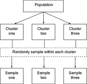
Fig. 5.20 Theoretical sample selection
5.6.4 Steps in Sampling Process
The major steps involved in sampling process are as follows:
- Define the population
- Sample frame identification
- Choose a sampling design or procedure
- Identify sample size
- Draw the sample
The major steps involved in the sampling process are discussed in Fig. 5.21.

Fig. 5.21 Sampling process
A quick comparison of random and non-random sampling is given in Table 5.3.
Table 5.3 Comparison of random and non-random sampling

Case Study
A survey is conducted to study “the communication behaviour of users in different educational levels”. Parameters selected in this study are as follows (Tables 5.4 and 5.5):
- People with UG, PG and PhD degree
- Males and females
- Sample size
Distribution matrix shows the particulars of population in percentage.

Table 5.5 Qualification table 2

We have to design quota sample in numbers as per the parameters which are
That is,
UG:PG:Phd = 4:7:9
Now Gender ratio ÷ Population
That is,
5.7 SPSS: A STATISTICAL ANALYSIS TOOL
SPSS is a software package released by IBM for statistical analysis of data. It is most commonly used in social science researches. Survey companies, marketing organizations and even government institutions make use of this package for efficient and fast data analysis. If we look the history of SPSS, it can be traced to 1968, where the SPSS Version 1 was released. Originally, SPSS stood for Statistical Package for the Social Sciences, but later it was modified to Statistical Product and Service Solutions. The first developers of SPSS were Norman H. Nie, Dale H. Bent and C. Hadlai Hull. It nearly took 15 years to have the next updated version, SPSSx-2. IBM acquired the SPSS package during the year 2009, and from there on six updated releases were made in the span of four years.
In general, we can express SPSS as a Windows-based program which is used to perform data entry and analysis. It handles large volume of data and can perform all sort of analysis in a very narrow time gap. SPSS looks like a spreadsheet similar to that of Microsoft Excel. All commands and options of SPSS can be accessed by the pull-down menus at the top of the SPSS editor window. This means, once you have learned the basic steps, it is very easy to figure out and extend your knowledge in SPSS through the help files. So, now let us look in detail how SPSS does the data analysis.
5.7.1 Opening SPSS
After installing the software, SPSS will be included in the IBM SPSS Statistics folder. There will normally be a shortcut on the desktop or we can access the software from the Start menu. Figure 5.22 shows the entire layout of SPSS.
Start Menu → All programs → IBM SPSS Statistics → IBM SPSS

Fig. 5.22 Layout of SPSS
Editor window of SPSS basically has two views, which can be selected from the lower left-hand side of the screen: the Data view and the Variable view. Data view is where you see the data that you are using. Variable view is where you can specify the format of your data when you are creating a file or while you load a pre-existing file. The default saving extension is .sav. But we can also import data through the Microsoft Excel. SPSS also has a SPSS Viewer window, which displays the output from any analyses that have been run. It also displays the error messages. Information from the Output Viewer is saved in a file with the extension .spo.
When prompted to open the software, you will see a pop-up window with a bunch of options. If you are new to SPSS, you can select the “Run the Tutorial” radio button on the right half of the dialogue box. If you want to analyze a dataset, you can choose either “type in data” or “open an existing data source” to select data from your computer. If your data file is shown in the list “More Files”, click the corresponding item and get it loaded. You can also add data files from the file menu, without disturbing the current data session. However, SPSS can only have one data file open at a time, so it is best to save the already opened data file before you try to open another one. Figure 5.23 details the screen shot while SPSS is being opened.
Now let us look how data is being loaded into the SPSS (Fig. 5.24). From the beginners’ point of view, we can load the data through Excel. Go to Files → Open → Data → Browse for the file. Once the data is loaded, the Editor window shows the loaded data and the output window will show the log details of the recently loaded data (Fig. 5.25).


Fig. 5.24 Loading data to SPSS

Fig. 5.25 SPSS after loading the data
After loading the data, if we want to see the details of the variables (Fig. 5.26) and its properties, we can go to the variable view in the Editor window. In our example, the variable view will be as shown in Fig. 5.27.
We can alter or add more variables from this variable view (Fig. 5.26). We need to double click the particular variable and a new dialogue box will be opened showing the various actions that can be performed at that particular step. The screenshot (Fig. 5.27) shows the variable properties of Name. The variable view of data always allows the user to understand the current statistics of the data snap-short.
5.7.2 File Types
Data files: A file with an extension of .sav is assumed to be a data file in SPSS for Windows format. A file with an extension of .por is a portable SPSS data file. The contents of a data file are displayed in the Data Editor window.
Viewer (Output) file: A file with an extension of .spo is assumed to be a Viewer file containing statistical results and graphs.
Syntax (Command) files: A file with an extension of .sps is assumed to be a Syntax file containing SPSS syntax and commands.


Fig. 5.27 Variable property
5.7.3 Analysis of Functions
There are more than 200 analysis functions available in the IBM SPSS-V21. All the analysis functions are very much user friendly and each output can be easily stored and exported. This makes SPSS globally acceptable. In this section, you are guided through two analysis processes: one sample T test (Fig. 5.28) and graph plotting. While you are working with the software, please try each data analysis option and see how quickly the process is taking place.

Fig. 5.28 Sample T test
One-sample t test
The one-sample t-test is used to determine whether a sample comes from a population with a specific mean. This population mean is not always known, but is sometimes hypothesized. So whenever this test is being done, the sample mean, variance, etc. could be easily calculated and the output is viewed in the output window. The steps for doing t test are explained in the figures. After loading the data to SPSS, you can select the t test from the Analysis tab. Figure 5.29 shows the output of one-sample t test.
Once the process is being run, it takes up to five seconds (depending on the bulkiness of data) to print the results in the output screen. The output can be saved in .spv format.
Graph representation
Now we can have another dataset for drawing/plotting the graph. There are various options to have pie chart, line graph, bar graph, scatter plotting, line plotting, etc. In this section, we are including how to get a scatter plot graph. The primary steps are the same as that of T testing. We need to open the data and load it. Now we need to take the option graphs from the menu bar and need to select the required type of graph, such as scatter, bar or histogram. Now select the x- and y-axis and then click on the start button. The out graph in .spv format will be available on the output screen. Figure 5.30 shows the output of the graph which was plotted. You can save or directly use the graph from the output screen.

Fig. 5.29 Output
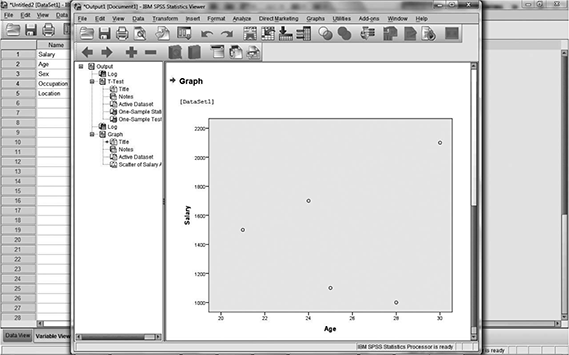
Fig. 5.30 Plotted graph
The aforementioned are two sample analyses that could be done with SPSS. For knowing the tool better, take a hands-on experience with IBM-SPSS Statistics.
EXERCISES
- What are the differences between Pearson correlation co-efficient and Spearman’s correlation co-efficient? At what condition a researcher select any one correlation co-efficient for the data analysis?
- Suggest an appropriate sampling design and sample size.
- Number of officials wants to estimate number of babies who are infected polio.
- Number of offices required support “Kissan Centre” by Government of India.
- The economic developer analyst wants to know educational bank loan and failure of loan recovery.
- Number of women scientists whose area of interest in marine science and its data collection.
- What do you mean by data analysis? Explain the various techniques used in data analysis.
- Define and differentiate regression analysis to correlation analysis.
- What do you mean by degree of correlation?
- How is PCA significant in data analysis?
- Explain in detail, strong–weak correlation.
- Explain the concept of population and sample in terms of sampling.
- What are sampling errors?
- What are the characteristics of a good sample design?
- In detail, explain the various types of sampling.
- Differentiate stratified and systematic random sampling.
- What are the various steps involved in sampling process?
- In detail, explain the various data analysis tools available.
- What are the various file types available in SPSS?
- Define one-sample t test.