Last week, Taila was carrying out a survey on the consumer demand for her tailoring shop, the Tailorie. Her boss wanted to know the spending habits of their customers. The customers would be classified by different age groups. She interviewed a dozen customers and came to the determination that middle-aged customers spent more money on fashionable clothes than young customers. However, her friend, who also interviewed a different dozen customers on the same issue, came up with the complete opposite results, that young customers spent more money on fashionable clothes than older ones. Today, she asked Prof. Metric to help explain the results. Prof. Metric responds that both of them might have selection-bias problems that caused the results to become unreliable. He says that this chapter will help us to solve the problem and once we finish the chapter, we will be able to:
1. Identify the selection bias problems.
2. Discuss the law of large numbers and balanced data in randomizedtrial experiments.
3. Explain the application of regression techniques into selection-bias correction.
4. Perform data analyses and interpret the results using Excel.
Identifying Selection Bias
Comparing Apples to Oranges
Prof. Metric tells us that Vu (2011) carried out a research on the difference between the income of graduates from public universities versus the income of graduates from private universities in the West Coast. We join him in looking at the survey results on 476 residents displayed in Table 10.1 and seeing that Panel 10.1 (a) displays the mean income of private-university graduates versus that of public-university graduates and their difference. The standard errors of the data analysis tell us that the private-university graduates earn more than the public-university graduates, and this difference is statistically significant.
Invo exclaims, “Oh, Panel 10.1 (b) tells us that most of the demographic characteristics are also statistically significant.” Prof. Metric says cheerfully,
Yes, the statistical significances of these characteristics imply that the high pay enjoyed by private university graduates might be due to their family backgrounds or their initial abilities in high school, instead of being the results of the better education they received at a private university. Hence there is evidence of a selection bias problem. In other words, we are going through a process of comparing apples to oranges instead of an apple-to-apple comparing process, which requires that only individuals from the same demographic group be compared to each other.
Table 10.1 Public versus private universities: Income and demographic characteristics
Variables |
Income |
||
Private University |
Public University |
Difference |
|
(1) |
(2) |
(3) |
|
Panel 10.1 (a) Income |
|||
Mean income |
$66,000 |
$46,000 |
$18,000 |
[12,340] |
[10,034] |
(3,132) |
|
Panel 10.1 (b) Demographic Characteristics |
|||
Parent years of education |
14.37 |
12.02 |
2.35 |
[1.24] |
[0.98] |
(0.34) |
|
Mean household income |
95,000 |
64,000 |
$31,000 |
[2,423] |
[1,870] |
(1,057) |
|
GPA in high school |
3.52 |
2.81 |
0.71 |
[0.38] |
[0.24] |
(0.13) |
|
Mean SAT score |
1,694 |
1,456 |
238 |
[182] |
[156] |
(29) |
|
Sample size: 476 |
|||
Note: The standard deviations are in the brackets, and standard errors are in parentheses.
Prof. Metric then tell us to look at Table 10.2, where an example of a two-student scenario is presented. The first student, Alpho, had a Grade Point Average (GPA) in high school of 3.41 and decided to attend a private university. He then had a cumulative GPA of 3.32 while completing his Bachelor of Business Administration (BBA) degree. The second student, Betal, had a GPA in high school of 2.51 and then decided to attend a public university. She had a cumulative GPA of 3.08 while completing her BBA. Assuming that a higher GPA at graduation represents a better education, we might be compelled to conclude that Alpho made a better choice by attending a private university.
However, it is misleading to say that Alpho is better off by attending a private university. From the table, Betal’s GPA increased 0.57 points from her high-school graduation to college graduation; whereas, Alpho’s GPA decreased by 0.09 points. Who knows what Alpho’s GPA could have become had he decided to attend a public university? Again, we are not comparing students from the same group. From the terminology of earlier chapters, we fail to hold other variables constant when we are comparing their GPA at the graduation, so there is a selection-bias problem.
Table 10.2 Public versus private universities: Two-student scenario
Students |
GPA |
||
Private University |
Public University |
Difference |
|
(1) |
(2) |
(3) |
|
Alpho |
GPA in high school |
3.41 |
|
GPA at graduation |
3.32 |
−0.09 |
|
Betal |
GPA in high school |
2.5 |
|
GPA at graduation |
3.08 |
0.57 |
|
Prof. Metric states that we will learn two techniques to correct the selection bias problem in this section. The first is to perform randomized-trial experiments, and the second is to use group dummies in multiple regressions.
Randomized-Trial Experiments
A randomized trial starts with a sample of the same group. In the preceding example, we can start with a group of high-school graduates of similar characteristics. A randomly chosen subset of this sample is then admitted to private schools (the treatment group) and let the rest go to public schools (control or comparison group). Later, the outcomes of the two groups can be compared.
Law of Large Numbers
Taila asks, “My friend and I did pick the survey list randomly. How is it that we still ended up with such different results?” Prof. metric praises her for a good question and says that a sample is only truly comparable if the group is large enough. In Table 10.2, there will be selection bias even if the two students are randomly picked among all students. In the previous example for a two-student comparison, Alpho is male and Betal is female. In this example, it is assumed that given the same amount of free or spare time, female students will usually spend a longer time working on their homework than their male counterparts. A sample of a dozen customers cannot be considered large enough, either. Hence, Taila and her friend should have interviewed dozens, if not hundreds, of customers each. That is, two randomly chosen groups, when large enough, are indeed comparable.
Booka asks, “Is the rule called the Law of Large Number (LLN)?” Prof. Metric says that she has picked the correct terminology. The LLN is a statistical property that characterizes the sample averages in relation to the sample size. For example, if you have roughly 300 customers, but you only calculate the average sale value of 10 customers, then the outcome will be very far from the true number. However, if we randomly pick sale values from 180 customers, then the average value will be much closer to the true sale value for 300 customers.
Checking for Balance
Prof. Metric emphasized that the sample not only needs to be large, but also should contain groups of similar characteristics to guarantee that we are comparing apples with apples. In the preceding example, the two subsets should bear similar demographic characteristics, except for the private or public university status. For example, we might want to pick a random sample from students with full scholarships to eliminate the income effect, or we might wish to pick a random sample from students that have similar GPA and SAT scores in high school to eliminate the initial-ability effect.
To make sure that the treatment and control groups are similar, a checking for balance process is performed. This comprises comparing the sample means as shown in Panel 10.1(b) of Table 10.1. From this table, the data are not balanced, that is, the characteristics are not the same, as evidenced by the mean differences between groups which are statistically different from zero. In other words, the data are considered balanced when there is no difference between the mean characteristics of the two groups.
Randomized Results
Prof. Metric tells us that Vu (2011) also carried out a randomized trial on the difference between income of graduates from public universities versus income of graduates from private universities in the West coast. He asks us to look at the survey results of 1,086 residents displayed in Table 10.3.
Panel 10.3 (b) shows the process of checking for balance of the data, including many groups with various demographic characteristics. From this table, the data are balanced because most of the differences are not significantly different from zero.
Panel 10.3 (a) shows the treatment effect of the random trial. Touro exclaims, “Oh, now the difference between income of the private university graduates and that of the public university graduates is no longer statistically significant.” Prof. Metric says that his observation is true. Hence, once the selection bias problem is corrected by a random trial, attending private universities does not improve a person’s income.
Table 10.3 Public versus private universities: Balanced data
Variables |
Income |
||
Private University |
Public University |
Difference |
|
(1) |
(2) |
(3) |
|
Panel 10.3 (a) Income |
|||
Mean income |
$55,000 |
$48,000 |
$4,000 |
[8,324] |
[6,647] |
(3,785) |
|
Panel 10.3 (b) Demographic Characteristics |
|||
Parent years of education |
13.37 |
12.23 |
1.14 |
[1.05] |
[0.78] |
(1.02) |
|
Mean household income |
75,000 |
69,000 |
$6,000 |
[2,103] |
[1,645] |
(3,257) |
|
GPA in high school |
3.06 |
2.94 |
0.12 |
[0.36] |
[0.28] |
(0.11) |
|
Mean SAT score |
1,595 |
1,532 |
63 |
[173] |
[164] |
(48) |
|
Sample size: 1,086 |
|||
Note: The standard deviations are in the brackets, and standard errors are in parentheses.
Group Dummies in Multiple Regression
In causal analysis, when randomized trials are not possible, either because LLN is not guaranteed or because the datasets are not balanced, multiple-regression inference is a reliable alternative. As emphasized in the previous chapters, the multiple regression method itself guarantees that we only make an interpretation of the change in the dependent variable due to a unit change in one explanatory variable, holding other variables constant. This is one step closer to obtaining equal means across other variables and partially solving the problem of selection bias. In addition, group dummies can be used in the manners similar to the ones in Chapters 4 and 6 to control for different characteristics among the groups.
Community College Versus University
Before discussing the regression method, Prof. Metric provides us with an example of Vu and Im (2015), who carried out research on the income of community college graduates versus four-year university graduates. The authors provide Table 10.4, which shows the distribution of average earning by education attainment in the United States. It appears that four-year university graduates earn substantially more than the community college graduates. However, is this observation true, once the opportunity cost of the two-year salary forgone while attending a university plus the financial costs incurred, for example, tuition, fees, room, and board, are accounted for?
To answer this question, authors first follow a nonregression approach of calculating the financial costs of attending two more years of university and the opportunity cost of the income foregone during those same two years is employed. Data for financial costs of attending a four-year university versus those accrued by attending a community college come from the College Board Annual Survey of Colleges website. In calculating the financial costs, they follow a conservative approach of assuming a low interest rate for student loans of 6 percent although the current rate is 7 to 8 percent. Students who do not have to borrow still face the same costs because the money paid toward the tuition, fees, room, and board can be invested somewhere else. The total difference for the time-horizon period is divided by the number of years to obtain the average per year difference between a four-year university and a community college.
Table 10.4 Mean earning by education attainment for U.S. residents (in U.S. dollars)
Education attainment |
2002–2004 |
2005–2007 |
2008–2010 |
|||
Level of highest degree |
Mean |
STDEV |
Mean |
STDEV |
Mean |
STDEV |
Not a high school graduate |
18,784 |
47 |
19,986 |
854 |
20,916 |
628 |
High school graduate |
27,330 |
562 |
29,721 |
1,236 |
31,065 |
380 |
Associate’s |
34,960 |
910 |
37,915 |
1,847 |
39,674 |
146 |
Bachelor’s |
51,008 |
333 |
54,344 |
2,634 |
57,486 |
1,009 |
Note: “mean” denotes average income per year, and “STDEV” is the standard deviation.
Source: U.S. Census Bureau.
In calculating the income foregone, they once again follow a conservative approach of using the past and current level of income, instead of expected future income. For example, the five-year horizon utilizes the average per year value of the past five years, instead of the expected income of the sixth year. The average per year income is then multiplied by the cost of attending two years of school, adjusted for the average return rate of investment, which again is chosen at 6 percent, and divided by the time horizon. The total sum of the financial and opportunity costs are then subtracted from the average per capita income.
The results are reported in Table 10.5. Prof. Metric reminds us to notice that for bachelor’s degree holders, the values in bold face denote those that are statistically lower than those of the associate’s degree holders, and the values in italics denote those that are statistically higher than those of the associate’s degree holders. The table reveals that the adjusted per capita incomes for the two levels of education are indeed not statistically different from each other for any time horizon between 9 to 12 years. For the time horizon less than nine years, the adjusted per capita income of a bachelor’s degree holder is statistically lower than that of an associate’s degree holder.
Table 10.5 Earning comparison for U.S. residents: Per capita income (in U.S. dollars)
Panel (a). Unadjusted earning |
||||||
Time horizon |
5-year |
8-year |
9-year |
12-year |
13-year |
14-year |
Associate’s |
36,143 |
37,632 |
37,867 |
38,286 |
38,798 |
38,798 |
Bachelor’s |
52,347 |
53,797 |
54,087 |
56,370 |
57,132 |
58,597 |
Panel (b). Adjusted earning |
||||||
Time horizon |
5-year |
8-year |
9-year |
12-year |
13-year |
14-year |
Associate’s |
36,143 |
37,632 |
37,867 |
38,286 |
38,798 |
38,798 |
Bachelor’s |
30,295 |
34,291 |
37,979 |
38,722 |
42,350 |
44,258 |
Difference |
−5,847* |
3,341* |
112 |
436 |
3,552* |
5,460* |
Note: * denotes 5 percent statistically significant.
From this table, it can be observed that not until the 13th year and after, do bachelor’s degree holders start to make statistically higher income than those of the associate’s degree holders, after adjusting for the costs of the two additional years in school.
Next, the authors used multiple regression analysis with a group of control variables. They employ an augmented Cobb–Douglas production function in logarithmic form similar to a “new growth model” in Barro (1991) or Romer (2006):
where PERCA denotes per capita income, ASPER is the ratio of the associate’s degree holders to the population, BAPER is the ratio of bachelor’s degree holders to the population. C is a vector of control variables that might affect the per capita income or employment rate, such as investment in physical capital, infrastructure, and so on. The error term ui is the fixed effect disturbance for state i, and the error term eit is the idiosyncratic disturbance.
Data on the numbers of associate’s and bachelor’s degrees conferred for all 50 states and Washington, District of Columbia, during the school years 2002 to 2010 are from the National Center for Education Statistics (NCES) website (https://nces.ed.gov/). Data for the school years 2002 to 2006 are from Table 301 on this website, “Number of degrees conferred in Title IV institutions, by award level, gender, and state.” Data for the school years 2006 to 2008 are from Table 335 on this website, “Degrees conferred by degree-granting institutions, by level of degree and state or jurisdiction.” Data for the school year 2008 to 2009 are from Table 332 on this website, “Degrees conferred by degree-granting institutions, by control, level of degree, and state or jurisdiction.” Data for 2009 to 2010 are from the “State Education Data Profiles,” also published by the NCES.
Data on the gross state products, employment, federal government expenditures on education, investment on physical capital, expenditures on medical facilities (as a proxy for health care), domestic trade, expenditures on transportation and warehousing (as a proxy for infrastructure), state and local government expenditures, household expenditures on education, information technology, and expenditures on social assistances for all 50 states and Washington, District of Columbia, during 2002 to 2010 are from the Bureau of Economic Analysis (BEA). All measures are in current dollars and therefore data on the price indices for GDP (implicit GDP deflators) from the BEA are used to convert them to real values. There are missing observations in the remaining data, so the authors have an unbalanced panel.
They start with all available variables to avoid omitted variables and performing the Variance Inflation Factors (VIF) tests on the possible multicollinearity as discussed by Kennedy (2006). After several rounds of the VIF tests to eliminate variables with VIF > 10, we end up with seven variables for analysis: LnASPER, LnBAPER, log of expenditures on social assistances (SOASI), log of infrastructure (INFRAS), log of information technology (INFOR), log of federal government expenditures on education (FEDAID), and log of investment on physical capital (INVEST).
The authors then performed the modified Hauman test and found that the variable LnBAPER had an endogenous problem: the p-value of the residual collected from regressing LnBAPER on all exogenous variables is 0.001, so a two stage least squares estimation is needed. Invo says, “I remember we discussed endogeneity in Chapter 7, and we used lagged variables as IVs.” Prof. Metric praised him for having a good memory and says that the authors regressed LnBAPER on all exogenous variables using the Blundell-Bond System Generalized Method of Moments (GMM) procedure as described in Bond (2002) to control for the lagged dependent variable problem. In the second stage, the predicted value of this regression (LnBAHAT) is used in lieu of LnBAPER in Equation (10.1).
Table 10.6 reports the estimation results for the fixed effect multiple regression without selective-group dummies. The authors also reported that an F-test performed on the null hypothesis showed that the difference of the estimated coefficients is zero, which yields a p-value of 0.1582. Invo says, “Oh, does that imply that the difference between LnASPER and LNBAHAT is not statistically different from zero?” Prof. Metric says that Invo’s remark is true and so two levels of education seem to affect per capita income with equal magnitude. He also reminds us that Equation (10.1) has the logarithm of earnings instead of earnings in levels. As explained earlier in this class, this allows the coefficient estimates to be interpreted as a percentage difference. For example, an estimated β = 0.1108 implies that a university school graduate earns 11.08 percent more than a high-school graduate.
Table 10.6 Results for estimations without selective-group dummies
Dependent variable: Log of Per Capita Income |
||||||
Variable |
Coefficient |
Standard Error |
t |
p-value |
[95% Conf. Interval] |
|
LnASPER |
.1594** |
.0338 |
4.72 |
.000 |
.0929 |
.2258 |
LnBAHAT |
.1108** |
.0245 |
4.52 |
.000 |
.0625 |
.1582 |
FEDAID |
.0043** |
.0016 |
2.62 |
.009 |
.0010 |
.0075 |
SOASI |
.0065 |
.0155 |
0.42 |
.673 |
.0369 |
.0239 |
INFRAS |
.0039** |
.0011 |
3.51 |
.001 |
.0017 |
.0061 |
INFOR |
.2457 |
.3248 |
0.76 |
.450 |
.3930 |
.8845 |
INVEST |
.0776** |
.0235 |
3.30 |
.001 |
.0313 |
.1239 |
Number of observations = 408
F( 59, 348) = 1184
Prob > F = .0000
RMSE = .0301
Note: ** denotes 1 percent statistically significant.
Since there is no difference in earning between community college and four-year university graduates, is it worth to spend that much more on obtaining a university education? The answer may not be that simple due to a variety of circumstances. The recent economic recession has caused high unemployment in many sectors of the U.S. economy and the resulting deterioration of household incomes. In the meantime, facing constraints in financial means, many firms are looking for job candidates with practical skills instead of possessing a deep knowledge in the liberal arts. The federal government and many state governments also seem to have shifted their attention and plans to give more favorable consideration in their distribution of financial aid to community colleges. For example, President Obama and many state governments were pursuing plans to finance free education to any student who decides to attend a community college. This raises the question of whether or not a four-year college education is still the staple of investment in human capital for most households in the United States.
Table 10.7 Total number of associate’s versus bachelor’s degree holders in the United States
Period |
2002–2004 |
2005–2007 |
2008–2010 |
|||
Region |
Associate |
Bachelor |
Associate |
Bachelor |
Associate |
Bachelor |
United States |
1894890 |
4040253 |
2160124 |
4487575 |
2524708 |
4649679 |
New England |
81084 |
262904 |
81125 |
285170 |
89356 |
294575 |
Mideast |
303661 |
734036 |
335245 |
805483 |
375972 |
827693 |
Great Lakes |
277937 |
685294 |
331640 |
742903 |
367297 |
760277 |
Plains |
153839 |
344630 |
180139 |
376616 |
198238 |
391666 |
Southeast |
444613 |
887434 |
513275 |
988830 |
596150 |
1032946 |
Southwest |
181629 |
390257 |
239885 |
458863 |
332486 |
484929 |
Rocky Mountain |
79297 |
167768 |
83190 |
190086 |
105757 |
195398 |
Far West |
372830 |
567930 |
395625 |
635936 |
427951 |
654991 |
Source: National Center for Education Statistics.
The authors also provide Table 10.7, which shows the descriptive statistics of the data on these two levels of education for the eight economic regions. The table reveals that the number of bachelor degree holders is more than twice that of associate degree holders. Hence, another question is: Does the United States really need so many university graduates to improve its living standard?
All aforementioned questions inspired the authors to perform another regression, in which they added eight group dummies to the estimated equation to control for the different characteristics among the U.S. eight regions:
where G is the group dummy variable. Prof. Metric offers further explanation: Giz indicates state i which belongs to region z. For example, i = 1 for Alabama, and z = 5 for the Southeast region, then Giz = G15 for this particular state.
Touro asks, “I forgot why we can use eight dummies for eight regions instead of just seven dummies.” Booka reminds him, “Equation (10.2) does not have a constant term, so we do not have to worry about a perfect collinearity between the sum of the dummies and the intercept.” We are all thankful to her for the reminder.
Table 10.8 Results for estimation with selective-group dummies
Dependent Variable: Log of Per Capita Income |
||||||
Variable |
Coefficient |
Standard error |
t |
p-value |
[95% Conf. Interval] |
|
LnASPER |
.1769*** |
.0403 |
4.39 |
.000 |
.0985 |
.2365 |
LnBAHAT |
.1102*** |
.0288 |
2.61 |
.010 |
.0601 |
.1497 |
FEDAID |
.0041*** |
.0014 |
2.93 |
.006 |
.0009 |
.0068 |
SOASI |
.0262* |
.0140 |
1.87 |
.062 |
.0247 |
.0438 |
INFRAS |
.0041*** |
.0015 |
2.73 |
.008 |
.0017 |
.0061 |
INFOR |
.2425** |
.1023 |
2.37 |
.018 |
.3724 |
.7853 |
INVEST |
.1537** |
.0462 |
3.05 |
.004 |
.9465 |
1.146 |
Number of observations = 408
F(59, 348) = 1012
Prob > F = .0000
RMSE = .0462
Note: *, **, and *** denotes 10, 5, and 1 percents statistically significant, respectively.
Table 10.8 reports the results for the model with this selection-control variable Giz. The authors again reported an F-test performed on the null hypothesis that the difference of the estimated coefficients is positive with the difference defined as D = LnASPER – LnBAHAT. The test result yields a p-value of 0.048 this time.
Taila exclaims, “Oh, so a community college graduate makes more money than a university graduate on average after the selective bias is controlled for.” Prof. Metric says that her remark is true at least for the first 10 years after they graduate. He also informs us that Vu, Hammes, and Im (2012) estimated a system of equation for 65 countries that also found that vocational education has a larger effect on economic growth than university education.
Data Analyses
Checking for Balance
Prof. Empirie tells us to go to the Data Analysis folder and click on the file Ch10.xls, Fig. 10.1, which provides data on household income as one of pretreatment demographic characteristics of the California residents, who participate in an experiment on the possible difference in health care expenditures as a percentage of income between construction workers and textile workers. The variable INCCON is Household Income of the Construction Workers, in thousands of dollars, and INCTEX is Household Income, of the Textile Workers, also in thousands of dollars. We are going to see if the pretreatment datasets are well balanced by performing a test on whether the mean of INCCON is equal to the mean of INCTEX.
Go to Data then Data Analysis.
Select “t-Test: Paired Two Sample for Means” then click OK.
In the box Variable 1 Range, enter B1:B31.
In the box Variable 2 Range, enter C1:C31.
In the box Hypothesized Mean Difference, enter 0.
Check the box Labels.
Check the button Output Range and enter E1 then click OK.
Click OK again to overwrite the data.
Figure 10.1 shows the results. Invo asks, “Is the t-statistic value in Cell F10?” Prof. Empirie says that he is correct and asks us to look for the t-critical in Cell F14. Touro says, “I think we do not need the t-critical value in Cell F12, because we are testing for equal means instead of greater or smaller, so only the two-tail value is relevant.” Prof. Empirie commends him for a keen observation and asks whether we can provide an interpretation of the results.
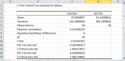
Figure 10.1 Testing for balanced data
Booka says, “Since the t-statistic is smaller than the t-critical, we fail to reject the null of equal means, so the datasets are well balanced.” Prof. Empirie praises her for the correct answer and directs us to the next empirical exercise.
Performing Multiple Regressions
Touro tells us that over the past nine years, his company has expanded its market to all 50 states and Washington, District of Columbia. Recently, his boss wanted to know how the profit (PROFIT) and the employment (EMP) of the company determine the investment (INV) level of the company. Touro tells us to click on the file Ch10.xls, Fig. 10.2-10.3. We notice that he also has two control variables, real interest rate (RINT) and stock of capital (CAP). We first perform a multiple regression without the selective-group dummies:
Go to Data then Data Analysis, select Regression then click OK.
The input Y range is E1:E460, the input X range is F1:I460.
Check the boxes Labels.
Check the button Output Range and enter R1 then click OK.
A dialogue box will appear, click OK to overwrite the data.
The results are displayed in Figure 10.2. From this table, EMP appears to have a much larger effect on the company’s investment than PROFIT.
Prof. Empirie then tells us to add seven dummies for seven economic regions so that we can perform a second regression with these selective-group dummies. Invo asks, “Since we have eight economic regions. Why do we need to only add seven dummies?” Booka answers, “I think we could add the eighth dummy if we suppress the constant term, which was not suppressed in the first regression.” Prof. Empirie praises her and says that we want to keep the constant term in this case for easy comparison between the two regressions. Here is what we do next:
Go to Data then Data Analysis, select Regression then click OK.
The input Y range is E1:E460, the input X range is F1:P460.
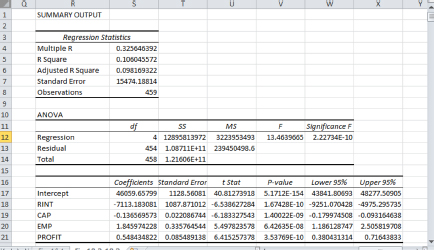
Figure 10.2 Results for regression without selective-group dummies
Check the boxes Labels.
Check the button Output Range and enter R25 then click OK.
A dialogue box will appear, click OK to overwrite the data.
The results are displayed in Figure 10.3. From this table, the coefficient estimate of EMP is much lower and not even statistically significant. Hence, there was a selection bias problem if the selective-group dummies were not added, and it turns out that EMP is not a determination of the investment level in Touro’s company.
Prof. Empirie then concludes that selection bias is a serious problem in econometrics, but one that can be corrected, with either randomized trials or multiple regressions with selective dummies added. Most of the time, the regression method is used because certain conditions for randomized trials are very difficult to satisfy.
Exercises
1. The file Income.xls provides data on household income as one of pretreatment demographic characteristics of South Carolina residents, who participated in an experiment on productivity disparity between community college graduates and four-year college (university) graduates. The variable HINC is Household Income of the Community-College Graduates in thousands of dollars, and HINU is Household Income of the University Graduates in thousands of dollars. Perform a test on the balance of the data.
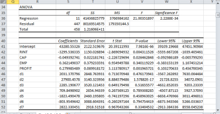
Figure 10.3 Results for regression with selective-group dummies
2. Table 10.9 provides the estimation results of an experiment in productivity mentioned in Question 1. Productivity is measured in thousands of dollars per worker.
a. Panel B shows the demographic characteristics of the dataset used for second estimation. Are the data in good balance? How do you know?
b. Give an interpretation of the first and the second estimation results concerning the difference between productivity of the university graduates and community college graduates, including the magnitudes, significance levels, and the implication of the results.
3. Continue with the same study in Exercises 1 and 2 on productivity comparison between community college graduates and university graduates. Equation (10.3) provides the regression results for a data analysis involving two groups of graduates. Group H includes five students from highly competitive schools of both levels (university and community college) and Group C includes four students from competitive schools also of both levels.
![]()
Table 10.9 Community college versus university: Randomized trials
Variables |
Means |
Difference between groups |
University |
(University–community college) |
|
Panel A. Productivity |
||
First estimation |
37.600 |
3.576 |
|
(1.002) |
|
Second estimation |
34.600 |
0.576 |
|
(0.548) |
|
Panel B. Demographic Characteristics |
||
Parent years of education |
11.55 |
0.82 |
|
(0.79) |
|
Household income |
50.89 |
3.89 |
|
(3.67) |
|
Sample size for first estimation: 15 |
||
Sample size for second estimation: 3,000 |
||
Note: The standard errors are in parentheses.
Table 10.10 Community college versus university: Regressions
Variables |
Column (1) |
Column (2) |
||
Coefficient |
p-value |
Coefficient |
p-value |
|
UNIV |
1.72 |
0.029 |
0.76 |
0.315 |
Log of household income |
0.198 |
0.043 |
0.192 |
0.046 |
Log of GPA |
0.102 |
0.032 |
0.099 |
0.039 |
Group dummies |
no |
no |
yes |
yes |
where PROD is productivity, the measured growth rate in percentage of output per worker, UNIV is a dummy variable, with UNIV = 1 for university graduates and UNIV = 0 otherwise.
a. What is the difference between the productivity of the community college and the university graduates concerning the magnitude and the significance level?
b. What could be the problem?
4. Table 10.10 provides results of the same study using the whole dataset of 867 graduates. Column (1) displays the estimated results with control variables added. Column (2) displays the estimated results with control variables and 29 group dummies.
a. What are the similarities and disparities between the results in the two columns regarding the magnitude and significant levels?