Appendix A

Basic Definition, Hysteresis and Eddy Current Losses

A.1 RESISTANCE AND RESISTIVITY

Resistance is the property of a substance due to which it opposes the flow of current through it. The unit of resistance is ohm (Ω).

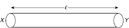
A conductor shown in Figure A.1 is taken length = l m and area of cross-section = a m².

If R is its resistance, we have

R ∝ l when a is constant.

R ∝ when l is constant.

R ∝ when both l and a are not constant.

Figure A.1

In Equation (A.1) ρ is a constant of proportionality, which is known as resistivity of the material.

If l = 1 m and a = 1 m², from Equation (A.1), we have R = ρ.

From Equation (A.1), we have

The unit of resistivity (ρ) is Ω–m.

A.2 INDUCTANCE

Usually, inductors are made of many turns of fine wire often wounded on a magnetic material that is capable of storing more energy, and it is property of one of the circuit elements by which energy is capable of being stored in magnetic flux field.

A.2.1 Self-inductance

The flux linked with the coil changes when the current in a coil is changing. In this case, an emf is produced in the coil. Let the permeability of the coil be taken as constant. The induced emf of the coil is proportional to the rate of change of current:

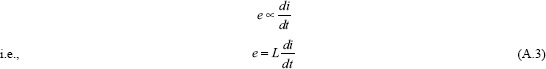
In Equation (A.3), L is the constant of proportionality, which is known as self-inductance of the coil. As per Faraday's law of electromagnetic induction, the induced emf in a coil is expressed by

where N is the number of turns of the coil.

From Equations (A.3) and (A.4), we get

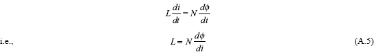
If Φ versus i graph is taken as linear, we have from Equation (A.5)

Since

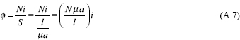
'S’ is the reluctance of the coil that is equal to

From Equation (A.7), we have

Using Equation (A.8), we have from Equation (A.6)

From Equation (A.9), we can conclude that inductance of any coil is dependent on its length and area of cross-section.

From Equation (A.6), self-inductance can also be defined as the flux linkage of the coil per ampere current flow through it. The unit of self-inductance is henry (H).

A.2.2 Mutual Coupling

Circuits become mutually coupled when the interchanging of energy takes place from one circuit to other. The coupling between the two circuits may be conductive, electromagnetic, or electrostatic.

A.2.3 Magnetic Coupling

The magnetic coupling has been shown in Figure A.2 in which a portion of magnetic flux established by one coil interlinks with the other. Hence, energy may be transferred from one circuit to the other through the medium of magnetic flux, which is common to both.

Figure A.2 Magnetic Coupling

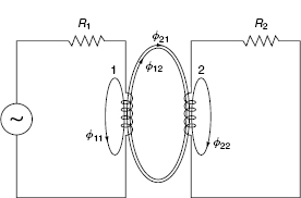
In Figure A.2, let Φ₁ and Φ₂ be the total flux established by V₁ and V₂, respectively.

Φ ₁ and Φ ₂ can be expressed as follows:

Φ₁ =Φ₁₁ +Φ₁₂     (A.10)

Φ₂ =Φ₂₁ +Φ₂₂     (A.11)

In Equations (A.10) and (A.11), Φ₁₁ and Φ₂₂ are the only fluxes that are linked to coil 1 and coil 2, respectively, whereas Φ₁₂ and Φ₂₁ in these two equations are the mutual fluxes that are linked to the turns of coil 2 and coil 1, respectively.

A.2.4 Mutual Inductance

The induced voltage in coil 2 due to a change in flux Φ₁₂ can be expressed by

Since Φ₁₂ is related to i₁, e₂ is proportional to the rate of change of i₁:

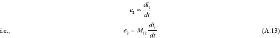
In Equation (A.13), M₁₂ is the constant of proportionality. It is known as mutual inductance between two coils, which is dimensionally equivalent to self-inductance L. The unit of mutual inductance is henry (H).

From Equations (A.12) and (A.13), we have

Also,

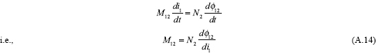
For linear variation of flux and current, we have the following from Equations (A.14) and (A.15):

and

Let the permeability of the mutual flux path be constant. We have M₁₂ = M₂₁ = M.

Therefore, the mutual inductance between two coils is defined as the weber-turns in one coil due to current through the other coil.

A.3 COEFFICIENT OF COUPLING

Coefficient of coupling gives an idea of how much of the flux produced by one coil is linking with the other; i.e., it indicates the extent to which the two inductors are coupled independently of the size of the inductor concerned.

Let the two inductive coupled coils 1 and 2 shown in Figure A.2 be the number of turns N₁ and N₂, respectively. The expression for inductance of coil 1 and coil 2 becomes

and

In Figure A.2, Φ₁ is the total flux established in coil 1 due to flow of current i₁ through it. If a part of it, i.e., Φ₁₂ = k₁Φ₁, is linked with coil 2, we have

where k₁ ≤ 1.

From Equations (A.20) and (A.21), we have

In Figure A.2, Φ₂ is the total flux established in coil 2 due to flow of current i₂ through it. If a part of it, i.e., Φ₂₁ = k₂Φ₂, is linked with coil 1, we have

If a fraction, k₂ ≤ 1, of this flux is linked with coil 1, then

From Equations (A.22) and (A.24), we have

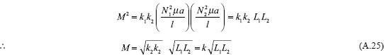
where k =

From Equation (A.25),

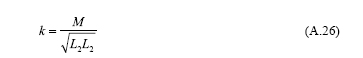
The constant k is known as the coefficient of coupling which has been expressed in Equation (A.26). The ratio of mutual inductance M to the square root of the product of inductance of coil 1 and coil 2 determines the value of k.

The coils are called tightly coupled or closely coupled, when the flux due to one coil is fully linked with the other. The value of k is unity in this case. If the flux in one coil does not link with the other coil, k = 0. The coils in this case are said to be magnetically isolated from each other or loosely coupled.

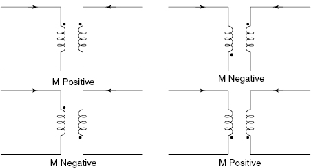
A.4 DOT CONVENTION

The emf induced due to mutual inductance may be aiding or opposing the emf induced due to self-inductance in a circuit, which totally depends on the relative directions of currents, i.e., the relative modes of windings of the coils as well as physical placement of one winding with respect to other. Using dot convention, the nature of mutually induced emf can be determined very easily. The actual mode of the winding is not required to show. Figure A.3 shows the sign of mutually induced emf.

Figure A.3 Dot Convention

A.5 INDUCTIVE COUPLING IN SERIES

If two inductors are coupled in series and mutual inductance exists between them, the equivalent inductance of this series coupling can be determined for series aiding and series opposing. This is explained below.

(i) Series Aiding

The connection of two coils in series aiding is shown in Figure A.4 when the flux produced by the two coils is additive in nature as per dot convention.

Let

• L₁ be the self-inductance of coil 1.
• L₂ be the self-inductance of coil 2.
• M is the mutual inductance between coil 1 and coil 2.

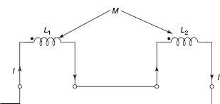
Figure A.4 Inductive Coupling in Series (Flux Aiding)

For Coil 1:

Mutually induced emf

[This is due to change of current in coil 2]

For Coil 2:

Mutually induced emf

[This is due to change of current in coil 1]

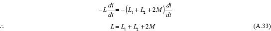
Therefore, the total induced emf of the above combination can be written as

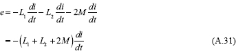
If L is the equivalent inductance of the coil, it can be written as

From Equations (7.31) and (7.32), we have

(ii)Series Opposing

Figure A.5 shows the coils which are connected in series. The fluxes or emfs are in opposite direction as per dot convention. Hence, the coils are said to be in series opposing.

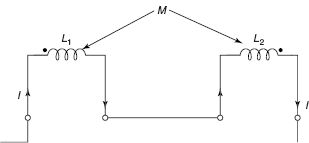
Figure A.5 Inductive Coupling in Series (Flux Opposing)

For Coil 1:

Mutually induced emf in coil 1 due to change of current in coil 2 can be written as

For Coil 2:

Mutually induced emf in coil 2 due to change of current in coil 1 can be written as

The total emf induced in the combination can be expressed as

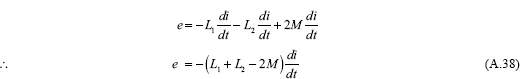
If L is the equivalent inductance of the combination, it can be written as

From Equations (A.38) and (A.39), we have

Therefore,

A.6 INDUCTIVE COUPLING IN PARALLEL

When two coils are coupled in parallel and mutual inductance exists, the equivalent inductance of the parallel combination can be determined for parallel aiding and parallel opposing as discussed below.

1. Parallel Aiding

   

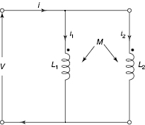
   Figure A.6 Inductive Coupling in Parallel (Flux Aiding)

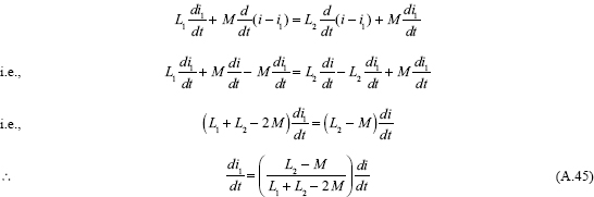
   The parallel connection of two coils is shown in Figure A.6. The flux is additive as per dot convention. Using KVL, we have

   

   and

   

   From Equations (A.41) and (A.42), we have

   

   Here, i = i₁ + i₂
   ∴  i₂ = i – i₁                                                                                                                (A.44)

   Using Equation (A.44), we have from Equation (A.43)

   

   Similarly,

   

   Using Equations (A.45) and (A.46), we have from Equation (A.41)

   

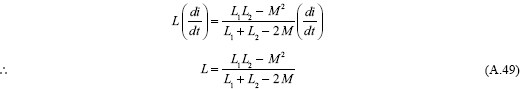
   Let L be the equivalent inductance of the parallel combination. We have

   

   From Equations (A.47) and (A.48), we have

   

   Equation (A.49) shows the equivalent inductance of Figure A.6.

   ii. Parallel Opposing

   

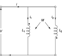
   Figure A.7 Inductive Coupling in Parallel (Flux Opposing)

   Figure A.7 shows the parallel connections of two coils when the mutually induced emf in one coil due to variation of current in other coil is negative.

   Using KVL, from Figure A.7, we have

   

   and

   

   From Equations (A.50) and (A.51), we have

   

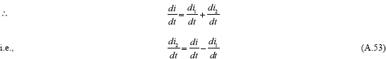
   Since  i = i₁ + i₂

   

   Using Equation (A.53), we have from Equation (A.52):

   

   Similarly, we have

   

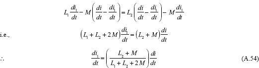
   Using Equations (A.54) and (A.55), we have from Equation (A.50):

   

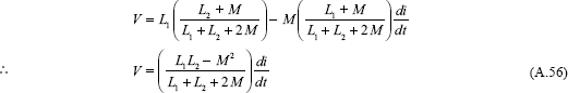
   If L is the equivalent inductance of Figure A.7, we have

   

   From Equations (A.56) and (A.57), we hav

   

A.7 AC OPERATION OF MAGNETIC CIRCUIT

DC sources are not used for excitation of magnetic circuit of transformers and other AC machines. AC sources are used. The steady-state current is calculated by the applied voltage and resistance of the circuit when DC excitation is applied. The inductance in this case plays the role only for the transient part. The adjustment of the magnetic flux takes place as per the value of current to satisfy the relationship of B–H curve or magnetization curve. For the case of AC excitation, inductance comes into picture for steady-state performance. The flux is determined by the impressed voltage and frequency. The adjustment of magnetization current takes place as per the value of this flux to maintain the relationship imposed by the magnetization curve.

Sometimes it is required to preserve the linear relationship of magnetization curve. Usually, the normal flux density in the magnetic circuit is out beyond the magnetization curve for the partial saturating circuit. Hence, it is difficult to get the accurate analysis on the basis of constant self-inductance. The equivalent parameters which remain substantially constant are used. From Faraday's law, we have

An iron core is considered which is excited by a winding having N turns carrying a current i. Let the magnetic flux (Φ) vary sinusoidally with time t as shown by the following relation:

In Equation (A.60), Φ_max and f are the maximum value of flux in the cycle and the supply frequency. The induced emf is expressed by

The rms or effective value of induced voltage is expressed by

The polarity of this induced emf is as per Lenz's law which opposes the change in flux. The induced emf leads the flux by an angle 90°. The applied voltage is opposed by the induced emf and the resistance drop. Usually, the resistance drop does not exceed a few per cent of the applied voltage in case of AC machines. Hence, resistance drop may be neglected. Therefore, the induced emf and the applied voltage are considered equal in magnitude. The value of Φ_max is determined from Equation (A.62).

A.8 HYSTERESIS AND EDDY CURRENT LOSSES

There are types of power losses in the form of heat in iron core when the magnetic circuits are subjected to time-varying flux densities. Theses losses cannot be neglected and have significance for determining heating, rating and efficiency of rotating machines, transformers and other AC-operated devices. The first loss is termed as hysteresis loss, which is associated with the phenomenon of hysteresis. Due to removal of the mmf, all the energy of the magnetic field is not returned to the circuit when the ferromagnetic materials are involved. The hysteresis loss is proportional to the area of the hysteresis loop and to the number of loops traversed per second when the variation of flux density is from +B_max to –B_max at the frequency f.

A.8.1 Determination of Hysteresis Loss

A ring of circumference l m and area of cross-section a m² having number of turns N of an insulated wire is considered here. The current through the wire is taken as I amperes. The magnetizing force is expressed by

If the magnetic flux density at this instant is B, the total flux through the ring is expressed by

If the current through the solenoid is alternating in nature, the emf induced is expressed by

The emf expressed by Equation (A.66) opposes the flow of current as per Lenz's law. If the source supply has an equal and opposite emf, it is possible to maintain the constant flow of current (I). Therefore, the applied voltage becomes

Figure A.8 Plot of B vs H

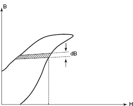
Figure A.8 shows the plot of flux density (B) and magnetizing force (H). A short interval dt is considered here, and the change of flux density at this time is also shown. Therefore, the energy consumed in this short interval is expressed by

Therefore, the total energy consumed during one complete cycle of magnetization is expressed by

In Equation (A.68), al represents the volume of the ring and H dB represents the area of elementary strip of B – H curve. ∫H dB is the total area of the hysteresis loop. Energy consumed per cycle is the product of volume of the ring and the area of the hysteresis loop.

The area of the loop is measured in units of H and B, i.e., ATΩm and WbΩm², to determine the hysteresis loss. The area of the loop is measured in square metre which is multiplied by the scales of H and B during measurement the area of the loop in units of H and B.

If 1 m represents p ATΩm on the H–axis and q WbΩm² on the B-axis, the hysteresis loss is expressed by

Using Steinmetz method, it is possible to determine the hysteresis loss. As per this method, the hysteresis loss per cubic metre per cycle of magnetization of a magnetic material is dependent on (i) the maximum value of flux density and (ii) magnetic quality of the material. Therefore,

where η is known as Steinmetz hysteresis coefficient which is a constant for each specimen, f is the frequency of reversal of magnetization and v is the volume of magnetic material in m³.

A.8.2 Determination of Eddy Current Loss

Because the core itself is composed of conducting material, voltage is induced in it due to the variation of flux. This induced voltage causes the circulating current in the iron known as eddy current. This current creates i²r loss which is known as eddy current loss. This loss is dependent on the rate of change of flux and the resistance of the path. Therefore, it can be taken as this loss varies as the square of the maximum flux density and the frequency and it is expressed by

where the constant K_e is known as eddy current coefficient and it is dependent on the type of core material, f is the number of complete magnetization cycles per second, B_max is the maximum flux density (WbΩm²), t is the thickness of laminations in metres, and v is the volume of core material in m³.

The core resistance must be increased to reduce the eddy currents. The magnetic cores are made of laminated thin sheets with an insulating layer (surface oxide or varnish) between successive laminations. Because eddy currents have magnetic effect, this makes the flux density at the centre lower compared to the surface which is known as screening effect. If the cores are properly laminated, this effect can be neglected at power frequencies. At high power frequencies, this effect may be significant.

These two losses altogether are known as iron loss or core loss. Core loss is present both in DC and AC machines.