Introduction

In the study of electrical machines the fundamentals of electromagnetism and single- and three-phase circuits play the most important role. The main aim of this introductory chapter is to introduce the basics, which are the cornerstones of electrical machines.

ELECTROMAGNETISM

When an electric current passes through a conductor, a magnetic field immediately builds up due to the motion of electrons. When a magnetic field encompasses a conductor and moves relative to the conductor, the electrons come in motion. This is the converse of the previous phenomenon. Electromagnetism is the study of electromagnetic force (emf) induced in the conductor when it cuts the magnetic flux or is cut by the magnetic flux.

DIRECTION OF CURRENT IN A CONDUCTOR

Figure 1(a) shows that there is no current through the conductor. Figure 1(b) shows that the conductor carries current away from the observer, that is, in a downward direction, while Figure 1(c) indicates that the conductor carries current towards the observer, that is, in an upward direction.

DIRECTION OF MAGNETIC FLUX IN A CONDUCTOR

The direction of magnetic flux can be easily found out by using either the right-hand rule or the corkscrew rule.

• Right-hand rule: If the conductor is graphed by the right hand in such a way that the thumb points in the direction of the current, then the closed fingers give the direction of flux, as shown in Figure 2.
• Corkscrew rule: Imagine a corkscrew is pointed in the direction of a current. The direction of magnetic field is in the direction in which the screw is to be turned to move it in a forward direction. The application of the corkscrew rule is shown in Figure 3.

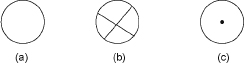
Figure 1 Direction of Current in a Conductor

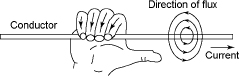
Figure 2 Right-hand Rule

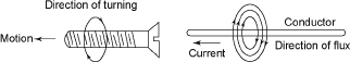
Figure 3 Corkscrew Rule

FLUX DISTRIBUTION OF AN ISOLATED CURRENT-CARRYING CONDUCTOR

The distribution of flux when a conductor carries current downwards, that is, away from the observer, is shown in Figure 4(a). The flux distribution when a conductor carries current upwards, that is, towards the observer, is shown in Figure 4(b).

FORCE BETWEEN TWO CURRENT-CARRYING CONDUCTORS

Figures 5(a) and 5(b) show the two conductors A and B, carrying current in the same and the opposite directions, respectively. The flux distribution when they carry current in the same direction is shown in Figure 5(a). The magnetic fields set up by the two conductors are in opposite directions. Hence, they attract each other. The flux distribution when they carry current in opposite directions is shown in Figure 5(b). The magnetic fields set up by the two conductors are in the same direction. Hence, they repel each other.

FORCE ON A CONDUCTOR IN A MAGNETIC FIELD

The force experienced by a current-carrying conductor placed in a magnetic field, shown in Figure 6, is expressed as

F = BIL

where F is the force on the conductor (N), B is the magnetic flux density (Wb/m²), I is the current in the conductor (A) and L is the effective length of the conductor to the field (m).

If F = 1N, I = 1A and L = 1 m, B = 1 T.

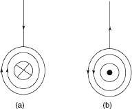
Figure 4 Isolated Current carrying Conductors

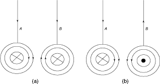
Figure 5 Two Current-carrying Conductors

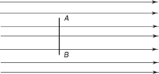
Figure 6 Conductor at an Angle of 90° to a Magnetic Field

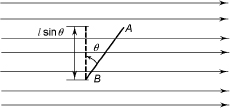
Figure 7 Conductor at an Angle θ to a Magnetic Field

If the conductor is placed at an angle θ to the field, as shown in Figure 7, the effective length will be L sin θ and the force on the conductor will be F = BIL sin θ.

The effective length is the length of the conductor lying within the magnetic field.

If θ = 0, that is, the conductor is placed parallel to the field, F = 0.

The basic principle of an electric motor is that the armature conductor carrying the current is placed in a magnetic field. So, it is also called the motor principle. The direction of rotation of the armature is defined by Fleming’s left-hand rule, as shown in Figure 8.

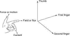
Figure 8 Fleming’s Left-hand Rule

Spread the thumb, forefinger and second finger of the left hand so that they are mutually perpendicular to each other. If the forefinger indicates the direction of flux and the second finger indicates the direction of current, the thumb will indicate the direction of rotation of the armature. Please see Appendix A for basic terminologies and losses.

GENERATION OF INDUCED EMF AND CURRENT

Figure 9 shows an insulated coil whose terminals are connected to a sensitive galvanometer (G). There is a bar magnet, AB, close to the coil. When the bar magnet is suddenly moved towards the coil to position A ‘B’, there is a deflection in the galvanometer. This deflection in the galvanometer lasts so long as there are relative motions of the magnet with respect to the coil; that is, the flux linking with the coil changes.

Figure 10 shows that when the magnet is withdrawn, the deflection of the galvanometer is in the direction opposite to the above case. This deflection exists so long as the bar magnet is in relative motion to the coil; that is, the flux linking with the coil changes.

Figure 9 Generation of Induced emf

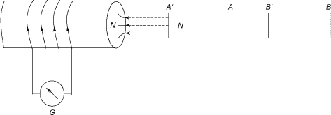
Figure 10 Magnet Withdrawn

In both the cases, the deflection is reduced to zero when the bar magnet becomes stationary. The flux linked with the coil increases as the bar magnet approaches the coil in the first case, while in the second case, the flux linked with the coil decreases when the bar magnet is withdrawn.

It is clear from above that deflections in the two cases are in different directions. The deflection in the galvanometer indicates that there is an induced current produced in the coil. In the first case, the induced current flows through the coil in an anticlockwise direction as seen from the bar magnet. This indicates that the face of the coil is the N pole. To move the bar magnet towards the coil, a force from outside must be given to the bar magnet. When the magnet is withdrawn, the current flows in a clockwise direction, as seen from the bar magnet. This indicates that the face of the coil is the S pole. So once again force must be supplied to the bar magnet from outside to take it away from the coil. Here, the principle of conservation of energy is fully satisfied.

From the above results, Faraday proposed two laws known as Faraday’s first and second laws.

FARADAY’S LAWS

• First law: Whenever there is variation of magnetic flux linked with a coil, an emf is induced in it. Or an emf is induced in a conductor whenever it cuts the magnetic flux.
• Second law: The magnitude of this induced emf is the rate of change of flux linkage.

Let the initial flux be Φ₁ and the final flux be Φ₂ in time t. Let the turns of the coil be N. Therefore, the initial flux linkage is NΦ₁ and the final flux linkage is NΦ₂.

In differential form, we can put Equation (1) as

LENZ’S LAW

The law states that the induced current will flow in such a direction that it will oppose the cause that produces it. It is explained as follows:

The current through the coil 1 is varied by the rheostat, as shown in Figure 11. An emf is induced in coil 2 due to variation of flux in coil 1. The induced emf between P and Q will be such that the current will flow from P to Q via the resistance R so that it will oppose the flux that is linked with it. In this case P will have a positive polarity and Q will have a negative polarity. The induced emf is given by .

Figure 11 Example of Lenz’s Law

INDUCED EMF

An emf is induced in the conductor either (i) dynamically or (ii) statically. In the first case, the conductor will move in the magnetic field and the flux will be non-varying. In the second case, the conductor will be stationary and the flux will be varying.

Dynamically Induced emf

In Figure 12(a), conductor A is shown by the cross-section within the uniform magnetic field. It moves at the right angle to the magnetic field of flux density B Wb/m². If the conductor moves a length dx in time dt, the area swept by it is equal to Idx, where l is the length of the conductor lying within the magnetic field. Here, change in flux is equal to Bldx in time dt. According to Faraday’s law, the induced emf (also known as dynamically induced emf) is expressed as

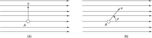
Figure 12 Dynamically Induced emf

where = the velocity of the conductor if the conductor moves at an angle Φ with the magnetic field shown in Figure 12(b). The component of its velocity in the direction perpendicular to the field is u sin Φ. The induced emf (e) becomes

If the conductor moves parallel to the field, the value of Φ will be 0°. The induced emf becomes zero; i.e., e = 0.

The direction of the induced emf can be found out by Fleming’s right-hand rule as shown in Figure 13. This rule states that if anyone spreads the thumb, forefinger and second finger of the right hand so that they are mutually perpendicular to each other, the thumb indicates the direction of rotation of the conductor in the magnetic field, the forefinger shows the direction of the magnetic field and the second finger indicates the direction of the flow of the induced current in the conductor.

Figure 13 Fleming’s Right-hand Rule

DC generators work on the principle of production of dynamically induced emf in the conductors, which are housed in a revolving armature lying within the magnetic field.

Statically Induced emf

If the flux in coil A varies by varying current with the help of the rheostat, the flux linked with coil B also changes and emf is induced in coil B, and its direction will be obtained by Lenz’s law.

Coil A is connected to a battery (E) via a rheostat (Rh) as shown in Figure 14. Coil B is connected to a voltmeter (V). When the current in coil A is established, the flux will be produced in coil A, and it varies by varying the current in the coil with the help of the rheostat. This varying flux links with coil B and emf is induced in the coil. This emf is also called mutually induced emf. In this case there is no movement of coil B. Similarly, if the connection is reversed, that is, a voltmeter is connected to coil A and the battery and the rheostat to coil B, the emf will be produced in coil A.

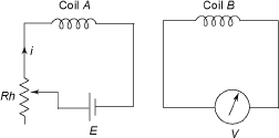
Figure 14 Statically Induced emf in Coil B due to Variation of Flux in Coil A

Another type of statically induced emf in a coil is the self-induced emf in a coil, which is produced due to the changes of flux in the coil itself by changing the current through it. In Figure 15, the current through the coil is changed by the rheostat (Rh). The flux linked with the coil also changes producing self-induced emf in the coil. The direction of the induced emf in the coil is obtained by Lenz’s law that opposes any change of flux in it. This emf is also known as opposing emf or counter emf.

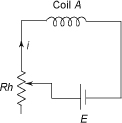
Figure 15 Statically Induced emf in a Single Coil

MAGNETIC CIRCUITS

Magnetic flux lines form closed loops. A magnetic circuit is defined as the closed path followed by flux lines. An electric circuit provides a path for electric current, whereas a magnetic circuit provides a path for magnetic flux. The knowledge of magnetic circuits is of utmost importance in the design, analysis and applications of electromagnetic devices such as transformers, rotating electrical machines and electromagnetic relays. The basics of magnetic circuits are introduced in the following sections.

MAGNETOMOTIVE FORCE

A current-carrying conductor produces a magnetic field around it. The coil should have the correct number of turns in order to produce the required flux density. Magnetomotive force (mmf) is defined as the product of current and number of turns.

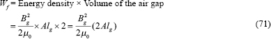
Magnetomotive force = Current × Turns

Let I be the current through the coil (A) and N be the number of turns in the coil.

The unit of mmf is ampere-turns (AT). Since N is dimensionless, its unit is ampere (A) also.

MAGNETIC FIELD INTENSITY

Magnetomotive force per unit length of magnetic flux path is called magnetic field intensity (H).

where l is the mean length of the magnetic circuit in metres. Magnetic field intensity is also called magnetic field strength or magnetizing force.

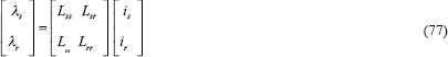
From Equation (5),

MAGNETIC FLUX

A current-carrying conductor produces a magnetic field around it. The magnetic field is measured in terms of flux lines (or simply flux) Φ and flux density B, the number of flux lines per unit area.

The density of flux is greatest near the conductor and tapers off inversely with distance.

The unit of flux Φ is webers (Wb) and the unit of magnetic intensity (B) is webers per metre square (Wb/ m²) or tesla (T).

1 weber = 10⁸

1 gauss = 1 Wb/cm² = 10^-4 Wb/m²

1 tesla = 10⁴ gausses

These units are in rationalized MKS system.

By Ampere’s law, the line integral of the field intensity around a closed path is equal to the current enclosed by that path.

The line integral of the closed path dl is the circumference of the circle 2πr.

From Equation (8),

From Equation (9) and (10),

i.e.,

For medium other than free space,

μ = μ₀μ_r

where μ_r is the relative permeability.

Flux is produced by current

Φ∝I.

If there are N turns instead of single conductor,

where NI, called ampere-turns (AT), is the flux-producing ability of the current-carrying circuit.

We can visualize NI or AT as the force that produces flux and hence is called the magnetomotive force, mmf (F).

Thus, we have arrived at a magnetic circuit similar to an electric circuit.

The medium surrounding the conductor causes resistance to the creation of flux. In the magnetic circuit, this resistance is called reluctance (S).

where S is the reluctance.

As in the case of an electric circuit, reluctance is directly proportional to length, l and inversely to area, A, and the property of the material called permeability, μ.

So, higher the permeability, lesser the reluctance and greater the flux.

We have seen that permeability of free space is very low, 4π × 10^-7 H/m. Ferromagnetic materials, that is, alloys of iron with cobalt, tungsten, nickel and aluminum, have very high permeability (μ_r), ranging from 2,000 to 80,000. High-permeability materials have the property of confining the flux within their cross-sectional area instead of spreading out as in space.

SINGLE-PHASE CIRCUITS

In AC circuits, voltage and current vary sinusoidally. The passive parameters of AC circuits are resistance (R), inductance (L) and capacitance (C).

Series R-L Circuit

Figure 16(a) shows an R-L series circuit.

Let

The current lags behind the voltage by an angle shown in Figure 16(b).

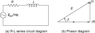
Figure 16 R-L Series Circuit

Here,

where X = ωL

Series R-C Circuit

Figure 17(a) shows an R-C series circuit.

Let

where I_m is the maximum value of current.

Where

where Z is called the impedance of the circuit.

The phasor diagram is shown in Figure 17(b). From Figure 17(b), the power factor of the circuit is given by .

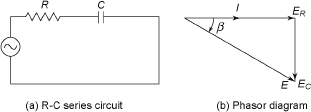
Figure 17 R-C Series Circuit and Its Phasor Diagram

Series L-C-R Circuit

Figure 18 shows a series R–L–C circuit.

Let

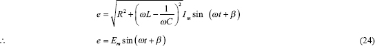
where

From Equation (25), the following conclusions can be drawn:

1. If β is positive. In this case the voltage leads the current by an angle β. The phasor diagram is shown in Figure 19(a).
2. If β is negative. In this case the current leads the voltage by an angle β. The phasor diagram is shown in Figure 19(b).
3. If In this case the voltage and the current are in phase. The phasor diagram is shown in Figure 19(c).

When β = 0, Z = R. The impedance is purely resistive and minimum. Whereas the current is maximum. This is the condition of resonance for a series resonance circuit.

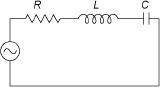
Figure 18 Schematic Diagram of Series R-L-C Circuit

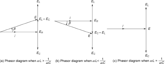
Figure 20 Phasor Diagrams of Series R-L-C Circuit for Three Different Cases

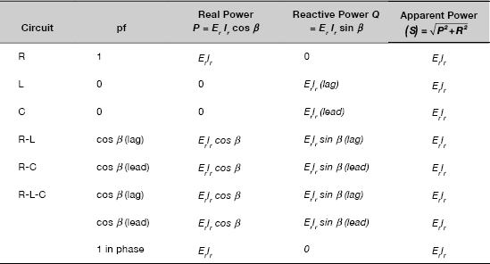
POWER TRIANGLE

The geometrical representation of apparent power, average power (true power or real power) and reactive power is called the power triangle. Figures 20(a) and 20(b) show power triangles for an inductive load and a capacitive load, respectively.

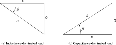
Figure 20 Power Triangles

COMPLEX POWER

S, P and Q of a power triangle can be obtained from the product VI. It is called complex power (S).

For a capacitive load, let

V = V_re^jθ and I = I_re^+j(θ+β)

i.e., S = VI* = V_re^jθ · I_re^-j(θ+β) = V_rI_re^-jβ = V_rI_r (cosβ – jsinβ)

= V_rI_r cosβ – j V_rI_r sinβ

i.e., S = P – jQ

Similarly, for an inductive load, let V = V_re^jθ and I = I_re^j(θ-β)

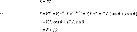
By convention, +Q indicates lagging reactive power while -Q indicates leading reactive power. The inductive load absorbs lagging reactive power and capacitive load supplies lagging reactive power. Table 1 shows the P, Q and S for different types of circuits.

Table 1 P, Q and S for Different Types of Circuits

THREE-PHASE CIRCUITS

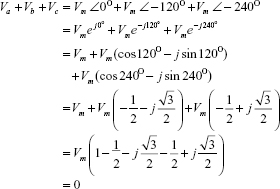
The generation of electrical power takes place in three phases in practice; these three phases are represented by a, b and c in Figure 21. The field rotates with synchronous speed. The three phases a, b and c are the armature conductors displaced from each other by 120° in a clockwise direction. With the position of the rotor shown in Figure 21 and the clockwise rotation of the pole, the emf induced in coil aa’ is maximum. The emf in conductor b of coil bb´ will be maximum when the pole turns through an angle 120° clockwise direction. Therefore, conductor b attains its maximum emf 120° later than the maximum emf in conductor a. Similarly, conductor c attains its maximum emf 120° later than the maximum emf in conductor b; in other words, 240° later than the maximum value in conductor a.

In this case the emfs induced in conductors a, b and c are equal in magnitude but 120° apart. The waveform and phasor diagrams are shown in Figures 22 and 23, respectively.

From Figure 23, we have

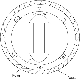
Figure 21 Generation of 3-phase Voltage

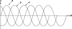
Figure 22 Waveform Diagram of Figure 21

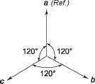
Figure 23 Phasor Diagram of Figure 21

The sum of Equation (26), (27) and (28) becomes

ADVANTAGES OF THREE-PHASE SYSTEM

The three-phase system has the following advantages compared to a single-phase system:

1. It is more economical as it requires less conductor material compared to a single-phase system.
2. A three-phase machine gives more output compared to a single-phase machine of the same size.
3. Three-phase motors have uniform torque, whereas most of the single-phase motors have pulsating torque.
4. Domestic power and industrial or commercial power can be supplied from the same source.
5. A three-phase motor produces more torque as compared to a single-phase motor.
6. Three-phase induction motors are self-starting, whereas single-phase motors are not self-starting.
7. Voltage regulation is better in a three-phase system.

PHASE SEQUENCE

The three phases may be denoted by a, b and c or R, Y and B where R, Y and B indicate red, yellow and blue, respectively. RYB has commercial usage. abc or RYB is taken as a positive sequence, whereas acb or RBY is taken as a negative sequence.

INTERCONNECTION OF THREE PHASES

The three separate armature coils of the three-phase alternator are shown in Figure 24.

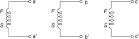
Figure 24 Three separate armature coils

STAR AND DELTA CONNECTIONS

The three armature conductors in a three-phase generator are not generally interconnected. They may be connected in the star (Y) or delta (A) form. The star connection of the three-armature conductors is shown in Figure 25 where all the similar ends a’, b’ and c’ are at the starting point. The terminals a’, b’ and c’ are joined to form the neutral terminal (N). In a star connection, similar ends are connected (the ‘s’ in star indicates similar ends). The neutral conductor may or may not be present. If it is present, it is called a three-phase four-wire system. Otherwise, it is a three-phase three-wire system. The delta connection of the three-armature conductor is shown in Figure 26. In a delta connection (the ’d’ in delta indicates dissimilar ends), dissimilar ends are interconnected.

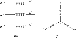
Figure 25 Star Connection

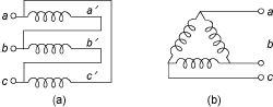
Figure 26 Delta Connection

VOLTAGES, CURRENTS AND POWER IN STAR CONNECTIONS

Figure 27 shows the three-phase three-wire system. The voltages V, V_b and V are called phase voltages, whereas the voltages V_ab, V_bc and V_ca are called line voltages, and the phase current (I_P) in each phase is equal to the line current in each line because each line is in series with its individual phase winding.

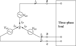
Figure 27 Star Connection of the Circuit

Let

V_P indicates the magnitude of phase voltage.

Now,

Similarly,

and,

Figure 28 shows the phasor diagram.

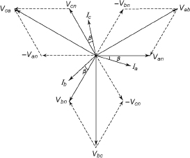
Figure 28 Phasor Diagram

So the magnitude of line voltage is times the magnitude of phase voltage. In this case, I_P = I_L. The active or true power in each phase of the circuit is given by V_p I_p cos β, where β is the angle between each phase voltage and its corresponding phase current. The total three-phase power (P) is expressed as

i.e.,

Similarly, total reactive power (Q) is expressed as

i.e.,

Q is positive when the load is of the inductive type, and it is negative when the load is of the capacitive type.

The total apparent power of the three phases

VOLTAGES, CURRENTS AND POWER IN DELTA CONNECTIONS

Figure 29 shows three voltage sources connected in delta. In Figure 29, the phase voltages and line voltages are identical, but the line currents and phase currents are not identical.

Here, taking I_ab as reference, we have

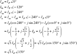
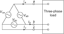
Figure 29 Delta Connection of the Circuit

Similarly,

and

The phasor diagram is shown in Figure 30.

From Figures 29 and 30, it can be seen that phase voltages are equal to line voltages. If I_P is the magnitude of phase current and I_L is that of line current,

then the total three-phase true or real power (P) is expressed as follows:

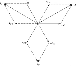
Figure 30 Phasor Diagram

The total three-phase reactive power (Q) becomes

Apparent power

For Star Connections

1. Phase voltage line voltage; delta connection phase voltage = line voltage. Thus, for a given phase voltage, Y, the connected alternator gives more line voltage and the insulation of the armature winding will not be costly.
2. As the star point is available in a star-connected alternator, the star point is connected to the ground. From the point of view of protection, it is advantageous.

   A practical connection is shown in Figure 31. The load is normally distributed among the phases in order to keep the system as balanced as possible.

   Here, suppose the line voltage is 400 V. The phase voltage to each domestic consumer will be Figure 31 shows that the domestic consumer (single-phase) as well as the industrial consumer (three-phase) can be supplied.

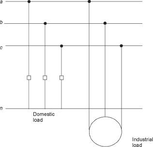
Figure 31 Connection of Domestic and Industrial Load

MEASUREMENT OF THREE-PHASE POWER

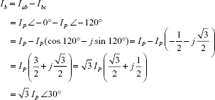
In this method, wattmeter W₁ is inserted in phase a and wattmeter W₂ is inserted in phase c. Their pressure coils are connected in phase b shown in Figure 32. Figure 33 shows the phasor diagram.

The sum of instantaneous power measured by W ₁ and W₂ is expressed as

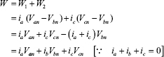
Therefore, W is the total instantaneous power of a three-phase circuit.

Figure 33 depicts a balanced load, and the currents in each phase lag behind the corresponding phase voltages by an angle θ from the phasor diagram; the current passing through the current coil of W₁ lags behind the line voltage V_ab by an angle 30° + θ. Similarly, the current passing through the pressure coil of W₂ lags behind the line voltage V_cb by an angle 30° – θ

Now, the magnitude of line voltage (V_L) is times the phase voltage V_P; that is, (V_L) = Let the value of current in each phase be I_P. So, the line current (I_L) = I_P. The line voltage magnitude V_L and line current I_L, are the rms values.

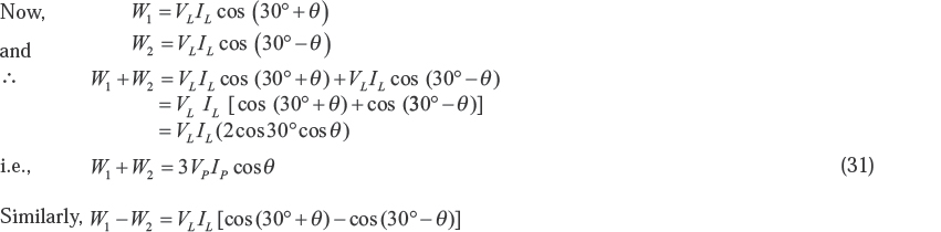
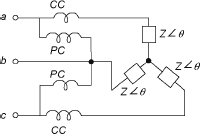
Figure 32 Two-wattmeter Connection

Figure 33 Phasor Diagram

Dividing Equation (32) by Equation (31), we have

i.e.,

Since W₁ = V_L I_L cos (30° + θ) and W₂ = V_LI_L cos (30° – θ) the following cases are discussed:

1. When θ = 0°, that is, the power factor is unity (resistive load), it can be written as W₁ = W₂ = V_LI_L cos 30°
   The readings of both wattmeters are equal in magnitude.
2. When θ = 60°, that is, the power factor = 0.5 lagging,
   W₁ = V_LI_L cos(30° + 60°) = V_LI_L cos90° = 0 and W₂ = V_LI_L cos(30° – 60°) = V_LI_L cos 30°. 0
3. When 90° > θ > 60°, the reading of W₂ is positive and that of W₁ is negative.
4. When θ = 90° (pure inductive load),
   W₂ = V_LI_L cos(30° – 90°) = V_LI_L cos (-60°) = V_LI_L cos 60° = V_LI_L sin 30°
   W₁ = V_LI_L cos(30° + 90°) = –V_LI_L sin 30°
   ∴W₁ + w₂ = 0

The above facts are for a lagging power factor load. For a leading power factor load, θ will be replaced by -θ in the expression of W₁ and W₂.

W₁ = V_LI_L cos(30° – θ)

and W₂ = V_LI_L cos(30° + θ)

During the experiment if any wattmeter shows a negative reading, it is necessary to reverse either its pressure coil or its current coil, usually the former. The reading of the wattmeter after the reversal of the pressure coil is to be taken as negative. In the above case, the abc phase sequence has been taken as positive.

PRINCIPLE OF ENERGY CONVERSION

The main aim of the principle of energy conversion is to estimate forces. The energy conversion can be neither created nor destroyed, but it can be converted from one form to the other. A typical electromechanical system is shown in Figure 34.

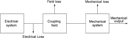
Figure 34 Electromechanical Energy Conversion System

The main parts of the system are as follows:

1. an electrical system,
2. a coupling field system and
3. a mechanical system.

The energy transfer equation is expressed as

The total energy losses in the system include I²R losses in the resistance of the winding of the electrical system, core loss in the field due to having of magnetic field in core as well as the mechanical loss in the form of friction and windage loss due to motion of mechanical components in the mechanical system. The total losses are converted into heat. Equation (34) becomes

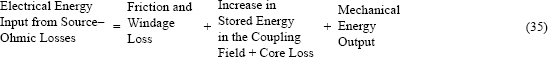
In differential form, Equation (35) becomes

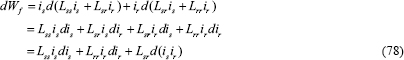
where dW_f represents change in energy stored in the field neglecting the core loss which is generally small and dW_m represents mechanical energy output when mechanical losses (friction and windage losses) are neglected.

ENERGY IN THE COUPLING FIELD

In rotating machines, the coupling field is the link between the stationary and movable members. In order to rotate the rotating member, an air gap must exist between the stator and the rotor. The energy stored in the coupling field must produce action on the electrical and mechanical system to ensure conversion of energy from electrical to mechanical (motoring mode) or from mechanical to electrical (generating mode).

In DC machines, the field system is a stationary member whereas the armature is a rotating member. For mechanical output (motoring mode), the coupling field must react with the electrical system to absorb the electrical energy from it. For electrical output (generating mode), the coupling field must react with the mechanical system to absorb mechanical energy from it. The reaction between the coupling fields with the electrical or mechanical system depends on the operating mode of the device. Since the torque (T) and the induced emf (e) are associated with the coupling field, it is termed as electromechanical coupling. Due to the inertia of the electromechanical coupling devices, these are slow-moving devices. Since the variation of the coupling field with time during energy conversion is slow, the electromagnetic radiation losses are neglected.

ENERGY IN THE FIELD

Figure 35 shows a simple electromechanical energy conversion system, which is a singly excited system because only one winding receives electrical energy.

A spring control is used to hold the movable part of the system in a static equilibrium. The movable part is held at an air gap ‘g’. The current in the winding is increased from 0 to i and hence the flux is established. Since the movable part is stationary, dW_m is zero and we have

Equation (37) indicates that all the electrical energy input is stored in the energy field because the core loss is neglected. For the flux linkage ‘λ’, the back emf induced in the winding becomes

The electrical energy input to the system is expressed as

From Equation (38) and (39), we have

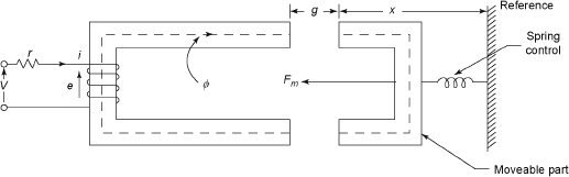
Figure 35 Electromechanical Energy Conversion System

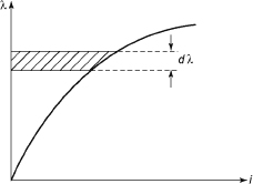
Figure 36 λ–i Characteristic for the System

where λ is increased from 0 to λ.

Figure 36 shows the relation between flux linkages and the current in the coil for Figure 35. The hatched portion of Figure 36 shows the incremental energy stored in the field. The total energy stored in the field is the space between X-axis and the curve (λ – i).

Let

N be the total turns of the system,

i be the input current,

H_c be the magnetic field intensity in the core,

H_g be the magnetic field intensity in the air gap,

l_c be the length of the magnetic core material and

l_g be the length of the air gap.

We have

If the cross-section area of the core material and uniform magnetic flux density are A and B, respectively, we have

i.e.,

Substituting dλ in Equation (41), we have

i.e.,

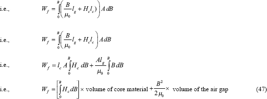
Let

W_fc be the energy density in the core

W_fg be the energy density in the air gap

V_c be the volume of the core material and

V_g be the volume of air gap.

Equation (47) becomes

The supplied energy to the system is partly stored in the magnetic field and partly in the air gap. The energy stored in the air gap is much larger than the energy stored in the field. The energy stored in the field is expressed as

CO-ENERGY

The magnetic material and the air gap length decide the flux linkage—the current characteristic of the electromagnetic system. The λ–i characteristic of the electromechanical system shown in Figure 35 is illustrated in Figure 37(a) for different air gap length. The characteristic becomes more linear when the air gap length is increased as shown in Figure 37(a).

From Figure 37(b), the energy stored in the magnetic field ’W_f'. is the hatched portion between the λ-axis and the λ–i characteristic. The hatched portion between the λ–i characteristic and the i-axis represents the co-energy (W'_f) of the system, which is used to estimate force or torque in an electromagnetic system as explained below. The co-energy (W'_f) of the system is expressed as

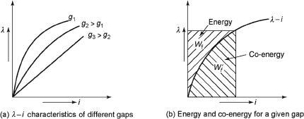
Figure 37 Co-energy

The total energy of the system is expressed as

Due to the non-linearity of the electromechanical system, co-energy is more than the energy stored in the magnetic field.

For linear systems,

ELECTRICAL ENERGY INPUT TO THE SYSTEM

A simple electromagnetic system with a single excited coil shown in Figure 35 is considered here. At any instant the terminal equation is represented by

In Equation (53), v is the instantaneous input voltage, i is the instantaneous input current and e is the back emf.

If λ is the instantaneous flux linkage, we have

Substituting ‘e’ in Equation (53), we have

From Equation (55), we have

iv dt = i² r dt + i dλ

i.e., i(v – ir)dt = i dλ

The elementary energy input to the system

We know that

where N is the total number of turns of the exciting coil and Φ is the instantaneous flux linking with the coil.

From Equation (56), we have

i.e.,

Most of the flux is confined to the core of the excited coil made of ferromagnetic material and the core extracts energy from the supply system for the case of change of flux linkage.

This change of flux causes the back emf that is responsible for extracting energy from the electrical system.

ESTIMATION OF MECHANICAL FORCES IN AN ELECTROMAGNETIC SYSTEM

Figure 38 shows the λ – i characteristic of the system when the moving part of the electromechanical system shown in Figure 35 is shifted from × = x₁ to × = x₂. The change of the λ – i characteristic shown in Figure 38(a) is for a system whose moving part moves very slowly and the excitation during this period of motion is assumed to be constant, whereas the λ – i characteristic shown in Figure 38(b) is for a system whose moving part is assumed to change its position very quickly. Let us consider the following cases.

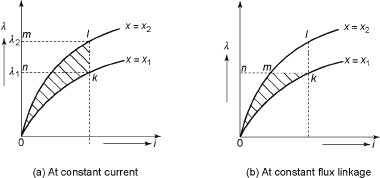
Figure 38 Locus of Operating Point on λ – i Characteristic

Case 1: Motion of the Moving Part Is Very Slow

For this case the excitation current is assumed to be constant during this period. When the moving part is shifted from x = x₁ to x = x₂, the λ – i characteristic moves upwards due to the decrease of the air gap length. The operating power in this case moves from k to l and the change of electrical energy during this case is given by

Energy stored in the magnetic field is expressed as

The mechanical work done by the moving part is expressed as

dW_m = dW_e – dW_f
= area klmn – (area olm – area okn)
= area klmn + area okn – area olm
= area okl
= hatched portion of Figure 38(a)

The shaded portion of Figure 38(a) represents the mechanical work done when the motion of the moving part is under constant current conditions which is also increase of co-energy and we have

If the mechanical force F_m, acts on the moving part to cause a displacement of dx, we have

F_m dx = elementary work done
=dW_m
=dW'_f

i.e.,

The force represented by Equation (63) acts on the moving part in such a direction so that it increases the stored energy of the system at constant current.

Case 2: Motion of the Moving Part Instantaneously

Figure 38(b) shows that the flux linkage with the exciting winding remains constant during the instantaneous motion of the moving part. The mechanical work done is represented by the hatched area okm and the field energy decreases. We have

F_mdx=dW_m=-dW_f

i.e.,

The negative sign in Equation (64) is due to decrease of the stored energy. During the instantaneous motion of the moving part, electrical energy input (dW_e) becomes zero due to the constant flux linkages. The requirement of mechanical energy output is met from the stored energy of the field, which causes the decrease of field energy. For small displacement, the area klm can be neglected.

ESTIMATION OF MAGNETIC FORCE IN LINEAR SYSTEMS

The reluctance of the magnetic path of the electromechanical system shown in Figure 35 is negligible compared to the air gap and hence the λ – i characteristic of the system becomes linear, causing the inductance to depend on the air gap.

From Equation (64), the magnetic force (F_m) is expressed as

For a linear system, energy is equal to co-energy and

From Equation (63), we have

Equation (68) and (69) show that the force obtained is the same. The entire mmf drop will be in the air path if the reluctance of the electromechanical system shown in Figure 35 is neglected. We have

The energy in the field is

From Equation (63), the magnetic force becomes

The force per unit area

DOUBLY EXCITED SYSTEMS

Figure 39 shows a rotatory electromagnetic system having the moving part known as the rotor. The fixed part of this system is known as the stator. Since the stator and rotor carry separate windings, this system is known as doubly excited system. The rotor is usually mounted on the shaft, which moves freely between the poles of the stator.

The rotor current I_r is fed through slip rings. I_s is known as stator current. Let e_s and e_r be the induced emfs in the stator and rotor windings. The energy stored in the magnetic field of the system for no mechanical output is expressed as

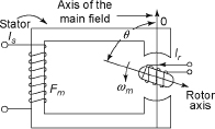
Figure 39 Rotatory Electromagnetic System Having the Moving Part

Equations (73) and (74) can be expressed in terms of inductances for linear systems. The inductances also depend on the position of angle of rotor (θ). We have the following expressions:

and

where L_ss is the self-inductance of the stator winding, L_rr is the self-inductance of the rotor winding and L_sr or L_rs is the mutual inductance between the stator and rotor windings. For linear systems, L_sr = L_rs, Equations (75) and (76) can be expressed as

Substituting λ_s and λ_r in Equation (74), we have

The total field energy is expressed as

i.e.,

The torque developed in the rotational system can be expressed as

In a linear system, since W_f = W´f

The first two terms in the right-hand side of Equation (80) are the torque due to the variation of self-inductance of the stator and rotor and are known as reluctance torque, whereas the third term is due to variation of mutual inductance between the stator and rotor windings. Please see Appendix B for Reluctance motor.

CYLINDRICAL ROTATING MACHINE

A cylindrical two-pole rotating machine consisting mainly of the rotor and stator is shown in Figure 40. They are provided with the distributed winding and assumed to be one slot/pole/phase for the sake of simplicity. If the effect of slots is neglected, the reluctance of magnetic path between the stator and rotor will be invariant. Let the inductance of the stator and the rotor windings be L_ss and L_rr, respectively.

Since L_ss and L_rr remain constant if the effects of the slots are neglected, no reluctance torque is produced. But due to variation in mutual inductance (L) between stator and rotor windings, the torque is given by

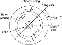
Figure 40 Cylindrical Rotating Machine

Also, L_sr = Mcos θ, where θ = ω_mt + δ, M is th emaximum value of mutual inductance between the stator and the rotor, ω_m is the angular velocity of the rotor, δ is the initial position of the rotor axis with respect to the stator axis at t = 0 and θ is the angle between magnetic axes of the stator and the rotor.

Let the instantaneous current in stator and rotor windings be

and

where ω = 2 πf_s and ω_r = 2πf_r.

Here, f_s and f_r are the supply frequency corresponding to the stator and rotor, and α is the phase difference between i_s and i_r. Substituting for i_s and i_r in Equation (81), we have

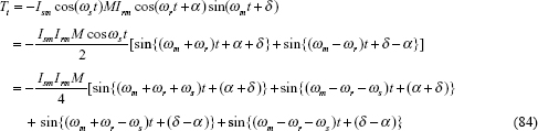
Equation (84) shows that instantaneous torque T_t' which varies sinusoidally with time. The average torque will be non-zero when the coefficient of t is 0.

Therefore, Motion of the Moving Part Is Very Slow

The above condition shows that the torque is developed in the machine when it runs at a speed equal to the sum or difference of synchronous speeds corresponding to the supply frequencies of rotor and stator currents.

Case 1: Synchronous Motor/Machine

In this stator, supply is three-phase balanced currents and rotor supply is DC current. Therefore, ω_r = 0, α = 0, ω_m = ω and I_r = I_dr.

The condition ω_m = ω_s indicates that the machine is rotating at synchronous speed corresponding to stator supply frequency. Substituting the above values in Equation (84), the expression is reduced as

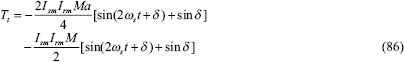
This instantaneous torque expression shows that the torque is pulsating in nature with non-zero average value. The average torque is

Equation (87) shows that when the rotor runs at a speed (ω_m = ω_s), the machine develops an average non-zero torque. The condition derived from Equation (84) also confirms that the synchronous motor is not self-starting when ω_m = 0. If the rotor is wound with single winding, it is called a single-phase synchronous motor. But due to pulsating field instead of rotating field, even though single-phase machine runs at synchronous speed, it produces noise and vibrations. This is eliminated by having three-phase winding on the stator.

Case 2: ω_m = ω_s – ω_r

When the stator and the rotor of the machine shown in Figure 40 carry AC currents at different frequencies, the motor runs at asynchronous speed ω_m = ω_s – ω_r. The instantaneous torque developed is obtained by substituting ω_m = ω_s – ω_r in Equation (84) as

The average value of this pulsating torque is expressed as

This is the torque developed in the inductor motor. In the three-phase induction motor, both stator and rotor currents are at different frequencies but the machine runs at synchronous speed. It has the self-starting torque.

When ω_m = 0, the average torque given in Equation (89) becomes zero, which is the same as that of the single-phase induction motor. To remove the nature of the pulsating torque, as given in Equation (88), the stator should carry three-phase winding as in the polyphase induction motor. Therefore, it can be concluded that the torque can be produced in rotating machines under two conditions: by variation in the reluctance of the magnetic path by rotating the rotor and by variation in mutual inductance between the stator and the rotor. But the torque that is produced is very small as in the case of the reluctance motor.

Example 1 For an electromagnetic system, the λ–i relation is given by (g = air gap length). Determine the mechanical force on the moving part of the system using

(i) energy of the system and

(ii) co-energy of the system.

Use i = 4 A and g = 5 cm.

Solution

i = 4 A, g = 5 cm and i.e., i = (λg)²

1. Mechanical force by using energy of the system
   
2. Co-energy of the system
   

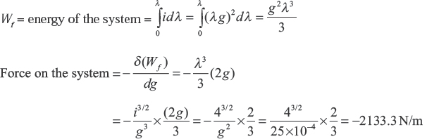
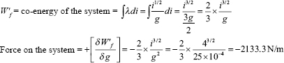
The negative sign in both the cases indicates that force acts in such a direction so as to decrease the air gap length.

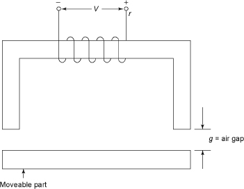
Example 2 The electromagnet shown in Figure E1 is wound with a coil which has 200 turns and a resistance of 2Ω. The air gap length is each of 5 mm and the magnetic core has a square cross-section of 2 cm × 2 cm. An average force of 300 N is required to lift the sheet of steel. For DC supply (1) source voltage and (2) energy stored in the magnetic field for 50 Hz AC supply. Determine the AC source voltage. Assume that the reluctance of core is negligible.

Solution

Given: F = 300 N, r = 2 Ω, g = 0.5 mm, A = 2 × 2 cm² and N = 200.

Energy in the air gap =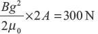

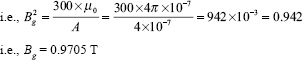
Figure E1

The mmf of the exciting coil = H_cl_c + H_gl_g

NI = 2 × (H_gl_g) since the core has zero reluctance

i.e.,

DC voltage source required = 7.72 × 2 = 15.44 V

Energy stored in the air gap = × volume of the air gap

(b) AC excitation:

Impedance of the coil = R + jωL

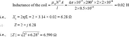
The rms value of the current in the coil = 7.72 A

AC voltage required = 7.72 × 6.59 = 50.87 V

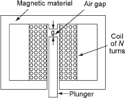
Example 3 A magnetic actuator is shown in Figure E2. The cross-sectional area of the plunger = 3 cm × 3 cm. The coil has 000 turns and a resistance of 5 Ω. A voltage of 12 V DC is applied to the coil terminals.

1. Assuming flux density in the air gap is 1.5 T. Determine the air gap g (in mm) and stored energy in the air gap.
2. Obtain an expression for the force on the plunger as a function of air gap length. Assume that the reluctance of magnetic material of the core is negligible.

Solution

Let x be the air gap at any time t where the plunger moves upwards in the direction of mmf and i be the current in the coil.

H_g = mmf in the air gap =

Figure E2

Inductance = flux linkage/current

Let A be the cross-sectional area of the plunger.

Φ_g = flux in the air gap = B_g × A

Ψ_g = flux linkages with the coil = NB_gA

L(x) = inductance of the coil =

Energy stored in magnetic field × volume of air gap

Force acting on the plunger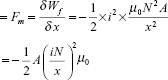

Mechanical work done by the plunger during motion:

Given: B_g = 1.5 T, N = 000, A = 9 cm², V_t = 1.2 V and R = 5 Ω.

Current through the coil = voltage/resistance

i.e,

Stored energy in the air gap

L(x) = inductance of the coil

Force acting on the plunger