D.1 Nonlinear Equation Solver <fsolve>

MATLAB has the built‐in function ‘fsolve(f,x0)’, which can give us a solution for a system of (nonlinear) equations. Suppose we have the following system of nonlinear equations to solve.

(D.1)

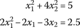
To solve this system of equations, we should rewrite as

(D.2)

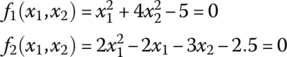
and convert it into a MATLAB function defined in an M‐file, say, ‘f_d02.m’ as follows.

Then we type the following statements into the MATLAB Command Window.

>>x0=[0.8 0.2]; % Initial guess [0.8 0.2]
>>x=fsolve('f_d02',x0,optimset('fsolve')) % with default parameters
  x = 2.0000  0.5000

If you see some warning message with the MATLAB solution obtained by using ‘fsolve()’ like this, you can change the value(s) of the optional parameters such as

• MaxFunEvals: Maximum number of function evaluations allowed
• MaxIter: Maximum number of iterations allowed
• TolFun: Termination tolerance on the function value
• TolX: Termination tolerance on x

by using the MATLAB command ‘optimset( )’ as follows.

 options = optimset('param1',value1,'param2',value2,...)

For example, if you feel it contributive to better solution to set MaxFunEvals and TolX to 1000 and 1e‐8, respectively, you need to type the following MATLAB statements.

>>options = optimset('MaxFunEvals',1000,'TolX',1e-8);
>>x=fsolve('f_d02',x0,options) % with new values of parameters
  x = 2.0000  0.5000

If you feel like doing cross‐check, you might use another MATLAB routine ‘Newtons( )’ which is defined in the next page.

>>x=Newtons('f_d02',x0) % Alternatively,
  x = 2.0000  0.5000

D.2 Differential Equation Solver <ode45>

Suppose we have a third‐order differential equation

(D.3)

We can rewrite this in a first‐order vector differential equation called a ‘state equation’ as

(D.4a)

(D.4b)

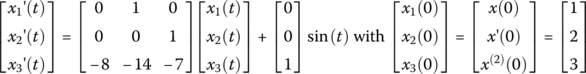
With this equation cast into a MATLAB function and saved as an M‐file named, say, “df_apd.m,”

we can type the following statements into the MATLAB Command Window to solve it:

>>[t,x]=ode45(@df_apd,[0 10],[1 2 3]); plot(t,x(:,1))
   % for time span [0,10]