Search in book...
Toggle Font Controls
Create new playlist

Name your new playlist

Playlist description (optional)
Sign In

Email address

Password

Forgot Password?

or

Continue with Facebook

Continue with Google
Sign Up

Full Name

Email address

Confirm Email Address

Password

or

Continue with Facebook

Continue with Google

Chapter 3

A Deep Dive into the Capture Phase

Abstract

This chapter describes the start of the CSRUD Life Cycle with initial capture and storage of entity identity information. It also discusses the importance of understanding the characteristics of the data, properly preparing the data, selecting identity attributes, and coming up with matching strategies. Perhaps most importantly, it discusses the methods and techniques for evaluating ER outcomes.

Keywords

Data profiling; data matching; benchmarking; truth sets; review indicators

An Overview of the Capture Phase

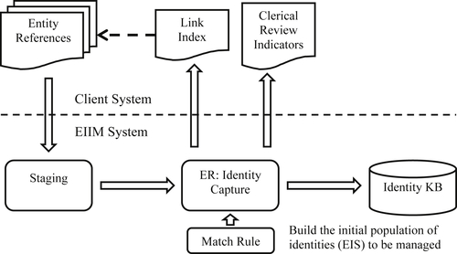
Figure 3.1 shows the overall flow of the capture phase of the CSRUD life cycle model. Entity references are placed into a staging area where they undergo data cleansing and data standardization based. Next they are processed by the ER engine implementing an ER algorithm and matching rule.

Each cluster of references the system determines are for the same entity is assigned a unique identifier. At the end of the process the cluster and its identifier are stored as an entity identity structure (EIS) in an identity knowledge base (IKB).

In addition to the IKB, the capture process has two other important outputs. One is the link index, and the other consists of the clerical review indicators. The link index is simply a two-column list. The items in the first column are the identifiers of the input, and the items in the second column are the EIS identifiers created during the capture process. Each row corresponds to one input reference where the first entry in the row is the unique identifier of the reference (from the client system), and the second entry is the identifier of the EIS to which the reference was assigned by the capture process. The link index is produced so that the client can append the entity identifiers to the original references for further processing within the client system.

Figure 3.1 Schematic of the capture phase.

For example, if the input references are enrollment records for students in a large school district, the link index would show which student (entity) identifier was assigned by the ER process to each enrollment record. If each record represents a different student, then all of the student identifiers would be different unless the ER process has made a false positive error. On the other hand, if two references have the same identifier, they may be positives because they represent the same transfer student between schools within the district.

The second output shown in Figure 3.1 is a list of review indicators. Review indicators are conditions or events that occurred during the ER process and alerted a data steward to the possibility of a linking error. As the name implies, review indicators should be manually reviewed by a data steward or other domain expert to determine whether or not an error was actually made or not. Just as important, if the person determines an error was made, then the system should provide some mechanism to help the person correct the error.

Review indicators represent an important aspect of ER and MDM data stewardship. They provide an important input into the update phase of the CSRUD life cycle. Unfortunately, review indicators along with formal ER results assessment are the two most neglected aspects of MDM implementations. The design and use of review indicators will be discussed in more detail as part of the update phase of the CSRUD life cycle in Chapter 5.

Building the Foundation

The CSRUD life cycle starts with the initial capture of entity identity information from entity references. Although the capture phase is a one-time process, it involves a number of activities that, if not done correctly, will hinder the future performance of the MDM system. The capture phase is similar to the design phase of a software development project: a critical first step laying the foundation for the entire system.

The key activities and steps for the capture phase are:

1. Assess the quality of the data

2. Plan the data cleansing process

3. Select candidates for both primary and supporting identity attributes

4. Select and set up the method or methods for assessing the entity identity integrity of the results

5. Decide on the matching strategy

6. Craft an initial data-matching rule

7. Run the capture with the rule and assess the results

8. Analyze the false positive and false negative errors and determine their causes

9. Improve the matching rule

10. Repeat Steps 6 through 9 until an acceptable level of error has been obtained.

Understanding the Data

The capture phase starts with a data quality assessment of each source. The assessment includes profiling the sources with a data quality profiling tool to understand the structure and general condition of the data and also visually inspecting the records in order to find specific conditions that may become obstacles to the ER process. The assessment will

• Identify which attributes are present in each source. Some attributes may be present in some sources, but not others. Even when the same attributes or types of attributes appear in two different sources, they may be in different formats or structured differently. For example, one source may have the entire customer name in a single unstructured field, whereas another source has the customer name elements (given name, family name, etc.) in separate fields.

• Generate statistics, such as uniqueness and missing value counts, that will help to decide which attributes will have the highest value as identity attributes. These are candidates for use in the matching rule.

• Assess the extent of data quality problems in each source, such as:

• Missing values, including null values, empty strings, blank values, and place-holder values, e.g. “LNU” for Last Name Unknown.

• Inconsistent representation (variation) of values whether due to inconsistent coding, such as “Ark” and “AR” as codes for “Arkansas” in the state address field, or due to inconsistent formatting, such as coding some telephone numbers as “(501) 555-1234” and others as “501.555.1234”. Here the most useful profiling outputs are value frequency tables, pattern frequency tables, and maximum and minimum values (outliers).

• Misfielding, such as a person’s given name in the surname field, or an email address in a telephone field.

Data Preparation

The next step is to decide on which data cleansing and standardization processes can be applied to address the issues found by the assessment. In the case where some files have combined related attribute values into a single unstructured field and others have the same information decomposed into separate fields, the first decision is whether to have a cleansing step attempting to parse (separate) elements in the unstructured field or combine the separate fields into a single field. The decision to parse unstructured fields will depend upon the complexity of the field and the availability of a parsing tool to accurately identify and separate the components. The decision to combine separate fields into one will depend upon the availability of a comparator algorithm able to effectively determine the similarity of compound, multi-valued fields.

The choice about combined versus parsed fields also ties to the larger issues of how much data preparation should be done prior to ER and how much should be handled by the ER process itself. Separating the data cleansing and transformation processes and making them external to the ER process may be simpler, but it also creates a dependency. If for some reason the data cleansing and transformation processes are not applied, or if they are applied differently at different times, an ER process running the same input data using the same match rule could produce dramatically different results. That said, moving data cleansing and transformation responsibility into the ER process tends to increases the complexity of matching rules, and if matching functions have more steps to perform, program execution times could increase. With the advent of faster and cheaper processors the trend has been to move more of the data cleansing and transformation processes into the ER matching process itself, thereby reducing the dependency on external data preparation processes.

Selecting Identity Attributes

One of the keys to success in any data quality project is an analysis to determine the critical data elements (CDEs) (Jugulum, 2014). For ER the CDEs are the identity attributes. Identity attributes are those attributes of an entity reference whose values are most helpful in distinguishing one entity from another. The values of some attributes provide the system with more power to discriminate among entities than other attributes. For customer references, name and address information, especially in combination, are often the primary basis for identification. However, other attributes can help confirm good matches or prevent unwise matches. For example, reliable gender information may prevent matching “J Smith (Male)” with “J Smith (Female)” for customers John and Jan Smith at the same address. In contrast, reliable telephone information might reinforce the decision to accept “John Smith, 123 Main St, 555-1234” with “John Smith, 345 Oak St, 555-1234” as the same customer even though the two references have different street addresses.

Primary identity attributes are those identity attributes whose values have the most uniqueness and completeness. For example, in the U.S. one of the most powerful discriminators for persons is the federally assigned unique social security number (SSN) for each individual. However, if a SSN is not present in the source, then it cannot be used in an ER process. Even in those cases where SSN might be present, such as school enrollment records, they do not always provide a perfect matching solution. Often SSN are erroneously reported or entered incorrectly into the system. Invalid values are sometimes deliberately entered when the data capture system requires a SSN value to be present, but the real value is not provided. Because it is rare that the values of one attribute will reliably identify all entities, in almost all cases, matching rules for entity references use a combination of identity attributes.

Supporting identity attributes are those identity attributes, such as gender or age, with values having less uniqueness or completeness. Supporting identity attributes are used in combination with primary identity attributes to confirm or deny matches. For example, in product master data the product supplier code is an attribute with possibly low uniqueness if many of the products under management come from the same supplier. In this case, the supplier code by itself would have limited discriminating power, but could still help to confirm or deny a match on other attribute values.

Three commonly used measures providing insight into the capability of an identity attribute to distinguish between entities include:

• Uniqueness

• Entropy

• Weight

Attribute Uniqueness

The uniqueness of an attribute in a given table or dataset is the ratio of the count of unique values to the count of all non-null values the attribute takes on. Most profiling tools automatically give uniqueness as a column statistic. If an attribute takes on a different value for every row or record of the dataset, then its uniqueness will be 100%. On the other hand, an attribute like student gender, which only takes on a few distinct values, will have an extremely low uniqueness value.

When assessing a set of references for primary and secondary attributes, it is important to remember the most desirable measure is not the uniqueness of the attribute’s values across all of the references, but the uniqueness of its values with respect to the entities the references represent. Assuming some redundancy in references, i.e. cases where different references in the set are referring to the same entity, then in those cases it is better if the attribute takes on the same value for equivalent references. In other words, if two references are for the same student, then having the same first name value in both references is a good thing even though it lowers the uniqueness of the first name attribute across the complete set of references. The most desirable feature of an identity attribute is the degree to which it has the same value for equivalent records and different values for nonequivalent references. The point is the level of uniqueness should be commensurate with the expected level of entity reference redundancy in the set of references. The actual measure for this is called the attribute weight as defined later in this section.

Attribute Entropy

Another measure often used to evaluate identity attributes is entropy as defined by Shannon (1948). Although similar to uniqueness, entropy takes into account the relative frequency of the unique values of an attribute.

$E n t r o p y = - \sum_{j = 1}^{n} {p r o b (v_{j}) \cdot \log_{2} (p r o b (v_{j}))}$ $E n t r o p y = - \sum_{j = 1}^{n} {p r o b (v_{j}) \cdot \log_{2} (p r o b (v_{j}))}$

In this formulation, the probability of a value (v_j) is its relative frequency in the dataset. In some ways, entropy is to uniqueness what standard deviation is to the mean in statistics. The more diverse the set of values an attribute takes on, the higher its entropy will be. In the case of an attribute having a constant value, the probability of that value will be 1, and because the log₂(1) = 0, the entropy of a constant value attribute will be 0.

Unlike uniqueness, the entropy value will vary with the distribution of values. For example, consider the gender attribute for a dataset comprising 100 references to students. If every reference has a non-null gender value of “M” or “F”, then the uniqueness measure will be 0.02 (2/100). However, the entropy measure will vary depending upon the distribution of values. For example, if there are an equal number of male and female students then the probability of “M” and “F” are both 0.5 (or 50%). In this case, the entropy of the gender attribute will be

$- (0.5 \cdot \log_{2} (0.5) + 0.5 \cdot \log_{2} (0.5)) = - (0.5 \cdot (- 1) + 0.5 \cdot (- 1)) = 1$ $- (0.5 \cdot \log_{2} (0.5) + 0.5 \cdot \log_{2} (0.5)) = - (0.5 \cdot (- 1) + 0.5 \cdot (- 1)) = 1$

On the other hand, if 70% of the students are female and 30% are male, then the entropy will be

$- (0.7 \cdot \log_{2} (0.7) + 0.3 \cdot \log_{2} (0.3)) = - (0.7 \cdot (- 0.515) + 0.3 \cdot (- 1.737)) = 0.882$ $- (0.7 \cdot \log_{2} (0.7) + 0.3 \cdot \log_{2} (0.3)) = - (0.7 \cdot (- 0.515) + 0.3 \cdot (- 1.737)) = 0.882$

Attribute Weight

Fellegi and Sunter (1969) provided a formal measure of the power of an identity attribute to predict equivalence, i.e. to discriminate between equivalent and nonequivalent pairs, in the specific context of entity resolution. Unlike uniqueness or entropy, the attribute weight takes into account the variation of an attribute’s values vis-à-vis reference equivalence.

To see how this works, suppose R is a large set of references having an identity attribute x. Further suppose S is a representative sample from R for which the equivalence or nonequivalence of each pair of references in S is already known. A sample set like S is sometimes called a Truth Set, Training Set, or Certified Record Set, for the larger set R.

If D represents all of the possible distinct pairs of references in S, then D = E∪N where E is the set of equivalent pairs in D, and N is the set of nonequivalent pairs in D. According to Fellegi and Sunter (1969), the discriminating power of x is given by

$\log_{2} (\frac{p r o b a b i l i t y (x v a l u e s a g r e e i n p a i r t | t \in E)}{p r o b a b i l i t y (x v a l u e s a g r e e i n p a i r t | t \in N)})$ $\log_{2} (\frac{p r o b a b i l i t y (x v a l u e s a g r e e i n p a i r t | t \in E)}{p r o b a b i l i t y (x v a l u e s a g r e e i n p a i r t | t \in N)})$

The numerator of this fraction is the probability equivalent pairs of references will agree on the value of attribute x, whereas the denominator is the probability nonequivalent pairs will agree on x. This fraction and its logarithmic value produce large positive numbers when the denominator is small, meaning agreement on x is a good indicator for equivalent pairs. In the case of equal probability, the ratio is 1 and the logarithmic value is 0. If agreement on x is more likely to indicate the pairs of references are nonequivalent, then the ratio is less than one and the logarithmic value is negative. The computation of the weight of an identity attribute is fundamental to a data-matching technique often referred to as “probabilistic” matching, a topic discussed in more detail later.

Assessing ER Results

If the goal of EIIM is to attain and maintain entity identity integrity (obey the Fundamental Law of ER), then it is important to be able to measure attainment of the goal. In ER this measurement is somewhat of a conundrum. In order to measure the degree of entity identity integrity attainment, it is necessary to know which references are equivalent and which are not equivalent. Of course if one already knew this for all references, then ER would be unnecessary in the first place.

Unfortunately, in many organizations the assessment of ER and EIIM results is done poorly if at all. ER and MDM managers often rely entirely on inspection of the match groups to see if the references brought together have a reasonable degree of similarity. However, as an approach to assessment, inspecting clusters for quality of match is inadequate in two fundamental ways. First, not all matching references are equivalent, and second, equivalent references do not always match.

Just inspecting clusters of matching references does not actually verify that the references are equivalent. Verification of equivalence is not the role of a matching expert; it should be done by a domain expert who is in a position to know if the references really are for the same real-world object. Furthermore, cluster inspection leaves out entirely the consideration of equivalent references not in the matching group under inspection, but that should be (Schumacher, 2010). These are references erroneously placed in clusters other than the one being inspected. In order to have a realistic assessment of ER results, the visual inspection of clusters should be replaced by, or at least supplemented with, other more comprehensive and systematic methods. Two commonly used approaches to this issue often used together are truth set development and benchmarking (Syed et al., 2012).

Truth Sets

A truth set is a sample of the reference for which entity identity integrity is known to be 100%. For a large set of references R, a truth set T is a representative sample of references in R for which the true equivalence or nonequivalence of each pair of references has been verified. This verification allows the references to be correctly linked with a “True Link.” In other words, two references in T have the same true link if and only if they refer to the same real-world entity. The true link identifier must be assigned and verified manually to make sure each cluster of references with the same true link value reference the same entity and that clusters with different true link values reference different entities.

Assessment using the truth set is simply a matter of performing ER on the truth set, then comparing the cluster created by the ER matching process to the True Link clusters. If the ER link clusters coincide exactly with the True Link clusters, then the ER process has attained entity identity integrity for the references in the truth set. If a cluster created by the ER process overlaps with two or more truth set clusters, then the ER process has produced some level of linking errors. Measuring the degree of error will be discussed in more detail later.

Benchmarking

Benchmarking, on the other hand, is the process of comparing one ER outcome to another ER outcome acting on the same set of references. Even though benchmarking is a relative measure, it is useful because most organizations trying to develop a new MDM system rarely start from scratch. Usually, they start with the known performance of a legacy system. Benchmarking is similar to the truth set approach because some previous ER result (set of clusters) is a surrogate for the truth set. The difference is, when a new ER grouping is compared to the benchmark grouping and overlaps are found, it is not immediately clear if the new grouping is more or less correct than the benchmark grouping, just that they are different.

Benchmarking is based on the following assumption: when both systems agree, those links are the most likely to be correct. This assumption allows the evaluation process to focus on references linked differently in the benchmark than in the new process. These differences must still be verified, but this method considerably reduces the review and verification burden. Where there are a large number of differences, a random sample of the differences of manageable size can be taken to estimate whether the differences indicate that the new process is making better or worse linking decisions than the benchmark.

Benchmarking and truth set evaluation are often used together because neither is an ideal solution. It is difficult to build a large truth set because of the need to actually verify the correctness and completeness of the links. An accurate truth set cannot be built by the visual inspection method. It requires verification by data experts who have direct knowledge of the real-world entities. For example, when managing student identities for a school system, the final determination whether the enrollment records are for the same student should be made by the teachers or administrators at the school the student attends.

Because truth sets tend to be relatively small, they may not include relatively infrequent data anomalies or reference configurations particularly problematic for the ER matching rule. The obvious advantage of the benchmark is that it can include all of the references in production at any given time. The disadvantage of the benchmark approach is its lack of precision. Even though links made by both systems are assumed to be correct, they may not be. Both ER processes may simply be making the same mistakes.

Problem Sets

Though not a method for overall assessment of ER results, collecting and setting aside problem references is another analysis technique commonly used to supplement both truth set and benchmark evaluation. Maydanchik (2007) and others advocate for the systematic collection of problem records violating particular data quality rules. In the case of ER, these are pairs of references posing particular challenges for the matching rule. These pairs of references are often collected during the creation of a truth set, when making a benchmark assessment, or from matching errors reported by clients of the system.

Even though the correct linking for problem reference pairs is known, it is usually not a good idea to incorporate them into the truth set. Ideally, the truth set should be representative of the overall population of the references being evaluated. If it is representative, then the accuracy of the ER process acting on the truth set is more likely to reflect the overall accuracy of the ER process. Even though it may be tempting to place the references in the problem set into the truth set to make the truth set larger, adding them can diminish the usefulness of the truth set for estimating the accuracy of the ER process. Adding problem records into the truth set will tend to skew estimates of the ER accuracy lower than they should be.

The Intersection Matrix

Whether using the truth set or the benchmarking approach, the final step of the ER assessment is to compare clusters created by the two processes running against the same set of references. Table 3.1 shows 10 customer references in a truth set referencing 4 entities (customers). These are the references having the True Link values “Cust1”, “Cust2”, “Cust3”, and “Cust4”. At the same time these records have been linked by an ER process with six link values of “5”, “36”, “43”, “56”, “66”, and “74”.

Applying links to a set of references always generates a natural partition of the references into a subset of references sharing the same link value. A partition of the set S is a set of nonempty, nonoverlapping subsets of S that cover S, i.e. the union of the subsets is equal to S.

Table 3.1

References with Two Sets of Links

	First Name	Last Name	Address	True Link	ER Link
R1	Mary	Smith	123 Oak St	Cust1	56
R2	Maria	Smith	456 Elm St	Cust1	56
R3	M	Smith	123 Oak Ct	Cust2	36
R4	Marilyn	Smith	765 Pine Rd	Cust2	36
R5	Mary Lynn	Smythe	873 Cedar Ln	Cust3	74
R6	M L	Smithe	237 Cherry St	Cust2	36
R7	Marie	Smith	45 Elm	Cust4	66
R8	Lynn	Smith	873 Cedar St	Cust3	74
R9	Mary	Smith	132 Oak	Cust1	43
R10	M	Smythe	237 Cherry	Cust2	5

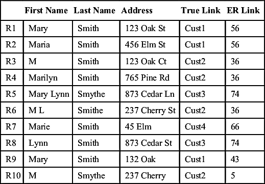
Using the example in Table 3.1, the True Link creates a partition T of S into 4 subsets where each subset corresponds to a unique link value

$T = {{R 1, R 2, R 9}, {R 3, R 4, R 6, R 10}, {R 5, R 8}, {R 7}}$ $T = {{R 1, R 2, R 9}, {R 3, R 4, R 6, R 10}, {R 5, R 8}, {R 7}}$

Similarly, the ER process creates a partition P of S having six subsets

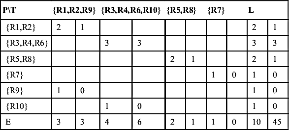
$P = {{R 1, R 2}, {R 3, R 4, R 6}, {R 5, R 8}, {R 7}, {R 9}, {R 10}}$ $P = {{R 1, R 2}, {R 3, R 4, R 6}, {R 5, R 8}, {R 7}, {R 9}, {R 10}}$

Therefore, the comparison of ER outcomes is essentially a problem in comparing the similarity between partitions of the same set. One way to organize the comparison between two partitions of the same set is to create an intersection matrix as shown in Table 3.2.

The rows of Table 3.2 correspond to the partition classes (subsets) of the P partition of the S created by the ER process. The columns correspond to the partition classes of the T partition created by the Truth Links. At the intersection of each row and column in Table 3.2 are two numbers. The first number is the size of the intersection between the partition classes in the case where there is a nonempty intersection. The second number is the count of distinct pairs of references that can be formed using the references in the intersection. This is given by the formula

Table 3.2

The Intersection Matrix of T and P

PT	{R1,R2,R9}		{R3,R4,R6,R10}		{R5,R8}		{R7}		L
{R1,R2}	2	1							2	1
{R3,R4,R6}			3	3					3	3
{R5,R8}					2	1			2	1
{R7}							1	0	1	0
{R9}	1	0							1	0
{R10}			1	0					1	0
E	3	3	4	6	2	1	1	0	10	45

$P a i r C o u n t = \frac{(N) (N - 1)}{2}$ $P a i r C o u n t = \frac{(N) (N - 1)}{2}$

where N is the number of references in the intersection.

The last row of the matrix is labeled E because it summarizes the counts of equivalent references and distinct pairs of equivalent references. For example, the second column has 4 equivalent references {R3, R4, R6, R10} that can form 6 pairs (4×3/2). Similarly, the last column is labeled L because it summarizes the counts of references linked by the ER process and possible pairs of distinct linked references. For example, the second row has 3 linked records {R3, R4, R6}, which can form 3 distinct pairs. The last number in the matrix is the total number of references (10) and the total number of distinct pairs that can be formed from all references (45).

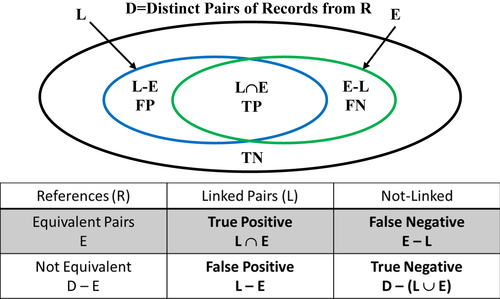
The intersection matrix in Table 3.2 can also be used to understand the distribution of true and false positives and true and false negatives. Let R be a set of entity references, and let D represent the set of all possible distinct pairs of references in R. In the example of Table 3.2, R has 10 elements and D has 45 elements. Following the Fundamental Law of Entity Resolution, the set D can be decomposed into four nonoverlapping subsets TP, TN, FP, and FN where

• TP is the set of True Positive resolutions. A pair of references belongs in TP if the references are equivalent and the ER process has linked them together.

• TN is the set of True Negative resolutions. A pair of references belongs in TN if the references are not equivalent and the ER process has not linked them together.

• FP is the set of False Positive resolutions. A pair of references belongs in FP if the references are not equivalent and the ER process has linked them together.

• FN is the set of False Negative resolutions. A pair of references belongs in FN if the references are equivalent and the ER process has not linked them together.

The Fundamental Law of ER holds when FP and FN are empty. Figure 3.2 illustrates the concepts represented as a Venn diagram.

The counts for each of these sets can be derived from the intersection matrix shown in Table 3.2. The pair counts at the nonempty cell intersections represent TP pairs because they are pairs of equivalent records now linked together. Table 3.2 shows the 5 true positive pairs in D.

$| T P | = 1 + 3 + 1 + 0 + 0 = 5$ $| T P | = 1 + 3 + 1 + 0 + 0 = 5$

The number of equivalent pairs (E) can be found by adding the pair counts in the last row.

$| E | = 3 + 6 + 1 + 0 = 10$ $| E | = 3 + 6 + 1 + 0 = 10$

Figure 3.2 The decomposition of D into FP, TP, FN, and TN.

Similarly, the number of linked pairs (L) can be found by adding the pair counts in the last column.

$| L | = 1 + 3 + 1 + 0 + 0 + 0 = 5$ $| L | = 1 + 3 + 1 + 0 + 0 + 0 = 5$

From these, all of the remaining counts can now be calculated as

$| F P | = | L | - | T P | = 5 - 5 = 0$ $| F P | = | L | - | T P | = 5 - 5 = 0$

$| F N | = | E | - | T P | = 10 - 5 = 5$ $| F N | = | E | - | T P | = 10 - 5 = 5$

$| T N | = | D | - | T P | - | F P | - | F N | = 45 - 5 - 0 - 5 = 35$ $| T N | = | D | - | T P | - | F P | - | F N | = 45 - 5 - 0 - 5 = 35$

Measurements of ER Outcomes

The TP, TN, FP, and FN counts provide the input for several ER measurements. The first is linking (ER) accuracy.

$L i n k i n g A c c u r a c y = \frac{| T P | + | T N |}{| T P | + | T N | + | F P | + | F N |} = \frac{5 + 35}{5 + 35 + 0 + 5} = 88.9 %$ $L i n k i n g A c c u r a c y = \frac{| T P | + | T N |}{| T P | + | T N | + | F P | + | F N |} = \frac{5 + 35}{5 + 35 + 0 + 5} = 88.9 %$

The accuracy measurement is a rating that takes on values in the (0,1) interval. When FP=FN=Ø, the accuracy value will be 1.0. If either FP≠Ø or FN≠Ø, the value will be less than 1.0. The accuracy calculation coincides with the Rand Index (Rand, 1971), which is also used in statistics to compare two clustering results.

The accuracy measurement incorporates the effects of both FP errors and FN errors in the same calculation. Often ER requirements put limits on each type of error independently and call for independent measurements. These typically are measured in terms of “rates.”

$F a l s e N e g a t i v e R a t e = \frac{| F N |}{| T P | + | F N |} = \frac{5}{5 + 5} = 50 %$ $F a l s e N e g a t i v e R a t e = \frac{| F N |}{| T P | + | F N |} = \frac{5}{5 + 5} = 50 %$

$F a l s e P o s i t i v e R a t e = \frac{| F P |}{| T N | + | F P |} = \frac{0}{35 + 0} = 0 %$ $F a l s e P o s i t i v e R a t e = \frac{| F P |}{| T N | + | F P |} = \frac{0}{35 + 0} = 0 %$

The false negative rate is the ratio of the actual number of false negatives (FN) to the total number possible. An ER process can only create a false negative error when it fails to link equivalent pairs of references. Therefore, the basis for the ratio is the total number of equivalent records E = TP∪FN (see Figure 3.2).

Similarly, the false positive rate is the ratio of the actual number of false positives (FP) to the total number possible. An ER process can only create a false positive error when it links nonequivalent pairs of references. Therefore, the basis for the ratio is the total number of nonequivalent records ∼E=TN∪FP (see Figure 3.2).

Three other commonly used measurements borrowed from the field of data mining are precision, recall, and F-measure.

$Linking Precision= \frac{| T P |}{| T P | + | F P |} = \frac{5}{5 + 0} = 100 %$ $Linking Precision= \frac{| T P |}{| T P | + | F P |} = \frac{5}{5 + 0} = 100 %$

$Linking Recall= \frac{| T P |}{| T P | + | F N |} = \frac{5}{5 + 5} = 50 %$ $Linking Recall= \frac{| T P |}{| T P | + | F N |} = \frac{5}{5 + 5} = 50 %$

$L i n k i n g F - M e a s u r e = \frac{2 (Precision \cdot Recall)}{Precision+Recall} = \frac{2 \cdot 1.0 \cdot 0.5}{1.0 + 0.5} = 66.7 %$ $L i n k i n g F - M e a s u r e = \frac{2 (Precision \cdot Recall)}{Precision+Recall} = \frac{2 \cdot 1.0 \cdot 0.5}{1.0 + 0.5} = 66.7 %$

These measurements think of linking as a classification operation in data mining. Linking precision looks only at reference pairs linked by the ER process, then asks what percentage of those were correct links. Precision is not affected by failure to link equivalent records (FN), focusing only on the correctness of the links that were made.

Conversely, recall is the measure of how many pairs of references that should have been linked (E) were actually linked by the process. Recall ignores improperly linking nonequivalent records (FP), focusing only on how many correct links were made. The F-Measure combines both precision and recall into a single measure by computing their harmonic mean.

Talburt-Wang Index

The Talburt-Wang Index or TWi is another measurement combining both FP and FN errors into one number (Hashemi, Talburt, & Wang, 2006; Talburt, Kuo, Wang, & Hess, 2004; Talburt, Wang et al., 2007). However, its computation is much simpler and does not require the actual calculation of the TP, TN, FP, PN counts. Instead it measures the number of overlaps between two partitions formed by different linking operations. In the TWi the size of the overlap is not taken into account, only the number of overlaps. If S is a set of references, and A and B represent two partitions of S created by separate ER processes, then define V, the set of overlaps between A and B as

$V = {A_{i} \cap B_{j} | A_{i} \cap B_{j} \neq Ø}$ $V = {A_{i} \cap B_{j} | A_{i} \cap B_{j} \neq Ø}$

Then the Talburt-Wang Index is defined as

$T W i (A, B) = \frac{\sqrt{| A | \cdot | B |}}{| V |}$ $T W i (A, B) = \frac{\sqrt{| A | \cdot | B |}}{| V |}$

Applying this to the truth set evaluation between sets T and P as shown in Table 3.2 gives

$T W i (T, P) = \frac{\sqrt{| T | \cdot | P |}}{| V |} = \frac{\sqrt{4 \cdot 6}}{6} = 81.6 %$ $T W i (T, P) = \frac{\sqrt{| T | \cdot | P |}}{| V |} = \frac{\sqrt{4 \cdot 6}}{6} = 81.6 %$

Two important characteristics of the TWi are

$0 < T W i (A, B) \leq 1.0$ $0 < T W i (A, B) \leq 1.0$

$T W i (A, B) = 1.0 i f a n d o n l y i f A = B$ $T W i (A, B) = 1.0 i f a n d o n l y i f A = B$

In the case A represents the partition formed by a truth set, then the TWi(A, B) is an alternative measure of linking accuracy.

The utility of the TWi is its simplicity of calculation, even for large data sets. Suppose that S is a set of references and that S has been partitioned by two linking processes, i.e. each reference in S has two link identifiers. If S is sorted in primary order by the first link identifier and secondary by the second link identifier, then the three values for the TWi can be calculated in one pass through the records. The overlaps are those sequences of references where both link identifiers are the same.

Table 3.3 shows the references from Table 3.1 sorted in primary order by True Link and secondary by ER Link. The alternate shading of the rows where both identifiers are the same indicates the 6 overlaps between the two partitions. If the number of unique True Links is known and the number of unique ER links is known from previous processing, then the TWi can be easily calculated by counting the overlap groups in the sorted file.

Other Proposed Measures

Two other proposed measures of ER outcomes are Pairwise Comparison and Cluster Comparison. These can best be explained by a simple example. Let

$R = {a, b, c, d, e, f, g, h}$ $R = {a, b, c, d, e, f, g, h}$

represent a set of 8 entity references. Furthermore suppose that the references in R have been resolved by two different ER processes, and that A and B are the resulting partitions of R formed by each process

Table 3.3

Table 3.1 Sorted by True Link Then ER Link

	True Link	ER Link
R9	Cust1	43
R1	Cust1	56
R2	Cust1	56
R10	Cust2	5
R3	Cust2	36
R4	Cust2	36
R6	Cust2	36
R5	Cust3	74
R8	Cust3	74
R7	Cust4	66

$A = {{a,c}, {b,e,f}, {d,g}, {h}}$ $A = {{a,c}, {b,e,f}, {d,g}, {h}}$

$B = {{a}, {b,c,e}, {f,d}, {g}, {h}}$ $B = {{a}, {b,c,e}, {f,d}, {g}, {h}}$

Menestrina, Whang, and Garcia-Molina (2010) proposed a pairwise method where “Pairs(A)” is the set of all distinct pairs within the partition classes. In this example

$Pairs (A) = {(a, c), (b, e), (b, f), (e, f), (d, g)}$ $Pairs (A) = {(a, c), (b, e), (b, f), (e, f), (d, g)}$

$Pairs (B) = {(b, c), (c, e), (b, e), (f, d)}$ $Pairs (B) = {(b, c), (c, e), (b, e), (f, d)}$

Then the pairwise measures are defined as

$PairPrecision (A,B) = \frac{| Pairs (A) \cap Pairs (B) |}{| Pairs (A) |} = \frac{1}{5}$ $PairPrecision (A,B) = \frac{| Pairs (A) \cap Pairs (B) |}{| Pairs (A) |} = \frac{1}{5}$

$PairRecall (A,B) = \frac{| Pairs (A) \cap Pairs (B) |}{| Pairs (B) |} = \frac{1}{4}$ $PairRecall (A,B) = \frac{| Pairs (A) \cap Pairs (B) |}{| Pairs (B) |} = \frac{1}{4}$

$pF (A,B) = \frac{2 \cdot PairPrecision (A,B) \cdot PairRecall (A,B)}{PairPrecision (A,B) + PairRecall (A,B)} = \frac{2}{9} = 0.222$ $pF (A,B) = \frac{2 \cdot PairPrecision (A,B) \cdot PairRecall (A,B)}{PairPrecision (A,B) + PairRecall (A,B)} = \frac{2}{9} = 0.222$

Menestrina et al. (2010) also proposed a Cluster Comparison method that is similar to Pairwise Comparison, but instead of using the Pairs() operator, it uses the intersection of the partitions, i.e. the partition classes A and B have in common. In the example given, the two partitions A and B only share the partition class {h}. Therefore

$A \cap B = {{h}}$ $A \cap B = {{h}}$

The Cluster Comparison measures are

$ClusterPrecision (A,B) = \frac{| A \cap B |}{| A |} = \frac{1}{4}$ $ClusterPrecision (A,B) = \frac{| A \cap B |}{| A |} = \frac{1}{4}$

$PairRecall (A,B) = \frac{| A \cap B |}{| B |} = \frac{1}{5}$ $PairRecall (A,B) = \frac{| A \cap B |}{| B |} = \frac{1}{5}$

$cF (A,B) = \frac{2 \cdot ClusterPrecision (A,B) \cdot ClusterRecall (A,B)}{ClusterPrecision (A,B) + ClusterRecall (A,B)} = \frac{2}{9} = 0.222$ $cF (A,B) = \frac{2 \cdot ClusterPrecision (A,B) \cdot ClusterRecall (A,B)}{ClusterPrecision (A,B) + ClusterRecall (A,B)} = \frac{2}{9} = 0.222$

Data Matching Strategies

Data matching is at the heart of ER. ER systems are driven by the Similarity Assumption stating:

“Given two entity references, the more similar the values for their corresponding identity attributes, the more likely the references will be equivalent.”

For this reason, the terms “data matching” or “record matching” are sometimes used interchangeably with “entity resolution.” Although there is usually a strong correlation between similarity and equivalence, it is not a certainty, only an increasing likelihood. As noted earlier, not all equivalent references match, and not all matching references are equivalent.

In order to really grasp the inner workings of MDM, it is important to understand that data matching takes place at three levels in an ER system:

1. The Attribute level

2. The Reference level

3. The Cluster level (or Structure level)

Attribute-Level Matching

At its lowest level, data matching is used to judge the similarity between two identity attribute values. A comparator is an algorithm that takes two attribute values as input and determines if they meet a required level of similarity. The simplest comparator determines “exact” match. If the two values are numeric, say age, then the two numeric values must be equal. If the two values are strings, say a person’s given name, then the two strings must be identical character-for-character. The problem with exact match is values encoded as character strings are prone to variation such as mistyping and misspelling. In exact match, even differences in letter casing (upper versus lower case) and spacing will not be an exact match.

In general, comparators are designed to overcome variation in representations of the same value. Therefore, in addition to exact match, other types of comparators provide either some level of standardization or some level of approximate match, sometimes referred to as a “fuzzy” match. This is especially true for comparators for values typically represented by character strings such as names or addresses.

What constitutes similarity between two character strings depends on the nature of the data and the cause of the variation. For example, person names may vary because names sounding the same may be spelled differently. The names “Philip” and “Phillip” have identical pronunciations and can easily be confused by someone entering the name on a keyboard during a telephone encounter such as a telemarketing sale. To address the variation caused by names sounding alike but spelled differently, a number of “phonetic” comparators have been developed such as the Soundex algorithm.

In this particular example, the Soundex algorithm will convert both the strings “Philip” and “Phillip” into the same value “P410.” This is done by first removing all of the vowels, then systematically replacing each character except the first character with a digit that stands for a group of letters having a similar sound.

Variation in string values caused by mistyping or other types of data quality errors are addressed by another family of comparators performing what is known as “approximate string matching” or ASM algorithms. One of the most famous is the Levenshtein Edit Distance comparator. It measures the similarity between two character strings as the minimum number of character delete, insert, or substitution operations that will transform one string into the other. For example, the edit distance between the strings “KLAUSS” and “KRAUS” is 2 because only 2 edit operations, the substitution of “R” for “L” in the first string and the deletion of the second “S”, are necessary to transform “KLAUSS” into “KRAUS”.

A more complete description of commonly used ER and MDM comparators can be found in Appendix A.

Reference-Level Matching

Most ER systems use one of two types of matching rules: Boolean rules or scoring rules. These are sometimes referred to as “deterministic” and “probabilistic,” respectively. However, these terms are somewhat of a misnomer because all ER rules are both deterministic and probabilistic. A process is said to be deterministic if, whenever given the same input, it always produces the same output. This is certainly true for all ER rules implemented as computer code because computer programs are, by nature, deterministic. In addition, all ER matching rules are probabilistic because the increasing similarity of two references only increases the probability they are equivalent. No matter how similar they are, there is still some probability they are not equivalent. Conversely, no matter how dissimilar two references, there is still a probability they may be equivalent. For this reason, they are referred to here as Boolean and scoring rules to make a clear distinction.

Boolean Rules

As the name implies, Boolean rules are logical propositions connected by the logical operators AND and OR (Figure 3.3). In the context of ER the logical propositions are that two values of an attribute meet a prescribed level of similarity.

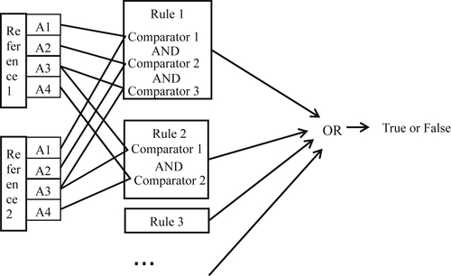
The two rules shown here are examples of a simple Boolean rule set potentially used in managing student enrollment data.

Rule 1:

(First: Soundex) AND (Last: Exact) AND (School_ID: Exact)

Rule 2:

(First: Exact) AND (Last: Exact) AND (Street_Nbr: Exact)

In Rule 1, the term “First” is the attribute of the student’s first name (given name), and the first name values are required to agree by the Soundex phonetic similarity algorithm. The term “Last” is the attribute representing the student’s last name (family name) and the “School_ID”, is an identifier for the student’s current school. In Rule 1, both “Last” and “School_ID” must be the same. Because each term is connected by an AND operator, all three conditions must hold in order for Rule 1 to be true, i.e. signal a match.

In Rule 2, “First”, “Last”, and the street number of the student’s address (“Street_Nbr”) must all be the same. However, the logical operation between rules is an implied “OR”. Therefore, if two references satisfy either Rule 1 or Rule 2 or both, the two references will be considered a match.

Scoring Rule

While Boolean rule sets can contain multiple rules comparing the same identity attributes in different ways, a scoring rule is a single rule that compares all the identity attributes at one time. Each comparison contributes a “weight” or score depending upon whether the similarity was satisfied (values agree) or not satisfied (values disagree).

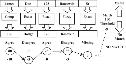
The diagram in Figure 3.4 shows an example of a scoring rule that compares five identity attributes of two customer references. The first name comparator is an alias or nickname match. The last name, street number, and street suffix require exact match, and the street name is a fuzzy match, such as Levenshtein edit distance. In this example, the first names agree by alias, the last names disagree by exact, the street numbers agree by exact, the street names agree by fuzzy match (e.g. Levenshtein edit distance <2), and one of the street suffix values is missing.

The score is calculated by summing the agreement and disagreement weights for each attribute plus the missing value weight for the street suffix, set at zero in this example. In this case, the total score for the match is 135. However, for this system the match threshold score has been set at 150. Therefore, the two references in this example are not considered a match.

The calculation of agreement and disagreement weights typically follows the Fellegi-Sunter (1969) model as discussed in the previous section on Attribute Weight. A more detailed description of weight calculation is covered later in the discussion in Chapter 8, “The Nuts and Bolts of Entity Resolution” and the Fellegi-Sunter Model is discussed in Chapter 7, “Theoretical Foundations.”

Hybrid Rules

Some systems implement matching rules that combine some characteristics of Boolean and scoring. One example is the use of an affinity scoring rule to supplement a set of Boolean rules (Kobayashi, Nelson & Talburt, 2011; Kobayashi & Talburt, 2013). The affinity scoring rule serves as a tie-breaker when a reference matches more than one EIS, but the EIS have been asserted (flagged) as true negatives to prevent them from being merged.

For example, two EIS are associated with twins in school that have similar information including same date-of-birth, same last name, same parent’s name, and same address. New references coming into the system often match both EIS by the base set of Boolean rules because they have such similar characteristics. Ordinarily when a reference matches two EIS, the system merges the two EIS due to transitive close. However, in the case where the EIS are known to be for different students, the EIS are marked as “do not merge” through a true assertion process discussed in more detail in Chapter 5.

The problem is due to the input reference referring to one of the twins, but the Boolean rules do not offer any help as to which one. When this specific situation arises, some systems then invoke a more granular scoring rule to determine which of the two EIS is a better match for input reference and should be merged with (Kobayashi & Talburt, 2014b).

Cluster-Level Matching

Beyond reference-to-reference matching, there is the issue of how to match a reference to a cluster or a cluster to another cluster. In general, the answer is the cluster is “projected” as one or more references or records, and the projected references are compared using a pairwise Boolean or scoring rule. The two most common projections of clusters are record-based projection and attribute-based projection.

A more detailed description of cluster projection and cluster-level matching is covered later in Chapter 8, “The Nuts and Bolts of Entity Resolution.”

Implementing the Capture Process

The actual implementation of the capture process starts by deciding on an initial Boolean or scoring match rule. In the case of a Boolean, it can be relatively simple and based on understanding and experience using the data. In the case of the scoring rule, the weights can be best guesses. The reason is because rule design is an iterative refinement process (Pullen, Wang, Wu, & Talburt, 2013b).

Starting with the initial rule and subsequent refinements, the results of using the rule must be assessed using either the truth set or benchmark methods discussed earlier to get an objective measure of false positive and false negative rates (Syed et al., 2012). Based on an analysis of these errors, the rule should be revised, run again, and assessed again. This process should continue until acceptable error rates are achieved. Once these levels are achieved, the residual errors can be addressed through a manual update process driven by the review indicators. The manual update process is discussed in more detail in Chapter 5.

Concluding Remarks

The CSRUD MDM Life Cycle starts with the capture phase. It is in this step that the match rules are iteratively developed and refined based on complete assessment of the reference data and careful measurement of entity identity integrity attainment at each iteration. Regardless of whether the system implements Boolean, scoring, or hybrid rules, ongoing ER assessment and analytics is critical. The investment in time to acquire or build proper ER assessment tools will be repaid many times, not only in the capture phase, but also for monitoring during the update phase.

..................Content has been hidden....................

You can't read the all page of ebook, please click here login for view all page.

Table of Contents for Chapter 3. A Deep Dive into the Capture Phase

Create new playlist

Sign In

Sign Up