From an analytical perspective, if X and Y represent the two lists, then the number of pairs to be considered for record linking will be |X|^∗|Y|, the size of the cross product X× Y. In merge-purge, there are (|X| + |Y|)^∗(|X| + |Y|−1)/2 pairs to consider. Moreover, in record linking, the maximum number of equivalences possible will be Minimum{|X|, |Y|} because each reference in List X can only be equivalent to, at most, one reference in List Y. If a reference in List X were equivalent to two references in List Y, then by transitivity of equivalence, the two references in List Y would necessarily be equivalent and contradict the assumption that no two pairs of references in List Y are equivalent. A similar argument holds that each reference in List Y can only be equivalent to, at most, one reference in List X.

However, the confusion is forgivable. Just from a practical viewpoint, starting an ER process with two lists where each list is known to be free of equivalent references is rare. Given two lists of references in the real world there could well be equivalent references within each list as well as between the two lists. As a practical matter, record linking is often implemented by first merging the two lists into a single list, then running a merge-purge or identity capture configuration. If the two lists are truly free of internal equivalences, then each cluster formed in the merge-purge process can comprise only a single reference or two references where each is from a different list. The latter indicates a link between the two lists. On the other hand, if a cluster contains two references from the same list, then the two references are presumably equivalent and this indicates the assumption was not justified. In this way, equivalence references can be found in one process both between the lists and within each list.

An agreement pattern between two references from Lists X and Y is an N-bit binary number where the k-th bit of the binary number represents the state of agreement between the k-th identity attribute of List X (x_k) and the k-th identity attribute of List Y (y_k). If the k-th bit of the pattern is a 1, then the two attributes agree in value. If the k-th bit of the pattern is a 0, then the two attributes disagree in value.

Take, as a simple example, two Lists X and Y sharing three identity attributes, say first name, middle name, and last name of a customer. Then the agreement patterns will be 3-bit binary numbers. For example, the agreement pattern 101 means the values of the first name attribute agree (1), the values of the middle name attribute disagree (0), and the values of the last name attribute agree (1). In this example of three identity attributes there are 8 = 2³ possible agreement patterns corresponding to the 8 binary numbers from 000 to 111. In general, for N corresponding identity attributes there will be 2^N possible agreement patterns.

It should also be noted that agreement does not necessarily mean the two identity attribute values are exactly the same. It could be defined to mean agreement on Soundex code, or having a q-Gram similarity of 80% or larger, or any other type of ER comparator. Moreover, agreement can be defined differently for each attribute.

In this respect, agreement patterns are a special type of Boolean match rule. In the previous example the 101 pattern might be interpreted as the proposition “(First name values agree on Soundex match) AND (NOT(middle name values agree by Exact match)) AND (last name values agree by Exact match)”. However, most systems supporting Boolean rules do not implement the NOT operator. Instead, the identity attributes not required to match are not specified in the rule and treated as “don’t care” states. In other words, the Boolean rule “First name values agree on Soundex AND last name values agree by exact” would be True as long there was agreement on the first and last name regardless of whether the middle name values agree or not. Thus, this Boolean version of the rule would encompass both the 101 and 111 Fellegi-Sunter agreement patterns.

Given two lists of references, List X and List Y, sharing N identity attributes, define Γ to be the set of 2^N possible agreement patterns. Then a Fellegi-Sunter matching rule is defined by three sets A, R, and V where

Although A, R, and V are nonoverlapping sets covering Γ, they do not always form a partition of Γ because they are not required to be nonempty subsets of Γ.

Now let x∈X, y∈X, and let γ∈Γ represent the agreement pattern between values of the identity attributes of the references x and y. Then the Fellegi-Sunter matching rule F = {A,R,V} states

All of this is just a mathematical way of saying divide all of the possible agreement patterns into three nonoverlapping groups, A, R, and V. When comparing references from Lists X and Y, if the values of the corresponding identity attributes conform to an agreement pattern in the set A, then the rule is to always link the references together. If the agreement pattern is in the set R, then the rule is to never link the references together. If the agreement pattern is in the set V, then the rule is a person must verify whether the two references should be linked or not.

The fundamental theorem of the Fellegi-Sunter theory says, given the context of two lists X and Y and constraints λ and μ, then it will always be possible to find a Fellegi-Sunter match rule F = {A, R, V} that is optimal with respect to the following:

Fortunately the proof of the theorem is a constructive proof, i.e. the proof of the theorem shows how to construct the rule F = {A, R, V} satisfying these conditions.

The construction starts with the two lists of references X and Y. Let X×Y represent all possible pairs of these references (x, y) where x∈X and y∈Y, and γ∈Γ is one of the agreement patterns. Now let E⊆X×Y represent the pairs of references actually equivalent to each other. The construction of the rule is fairly straightforward and relies primarily on the following formula:

The fraction R_γ is called the Pattern Ratio for pattern γ. The numerator of the ratio is the probability two equivalent references will conform to the agreement pattern γ, and the denominator is the probability that two nonequivalent references will conform to γ. Because these fractions can be very large or very small, the theorem also defines W_γ the Pattern Weight for γ by simply converting the ratio R_γ to its logarithmic value, i.e.

The pattern ratio and pattern weight measure the predictive power of each pattern for equivalence or nonequivalence. If the probability that equivalent references satisfy a given pattern is high and the probability that nonequivalent references satisfy the same pattern is low, the ratio will be very large. It also means the pattern is a good predictor of whether the two references should be linked because it is associated with a high probability of equivalence, thus creating a true positive link. As the numerator approaches 1 and the denominator approaches 0, the value of the ratio becomes unbounded. To avoid the problem of division by zero, the denominator is never allowed to be smaller than a very small, but fixed, value.

On the other hand, if the numerator is small and the denominator is large, the ratio will be small and weight will be a small negative value. In this case the pattern predicts that the references should not be linked because the references are more likely to be true negatives.

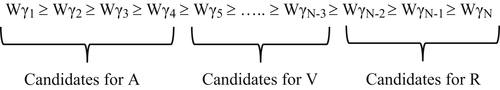
From this it is easy to see that the highest weight patterns are the best choices for members of the set A of the rule (always link), and the lowest weight patterns are the best choices for members of the set R of the rule (never link). In the proof of the theorem the patterns are ordered from highest to lowest weight.

The ordering and candidates for the members of the A, V, and R set of the rules are shown in Figure 7.1. The only question is how many of the patterns with high weights should go into A and how many with the lowest weights should go into R. The answers to these questions are determined by the constraints λ and μ.

Note that if a pattern is selected for the set A, then any pair of references conforming to the pattern will be linked. Linking will either result in a true positive or a false positive. Patterns in A never create false negative links. They can only make true or false positives. Also, unless the denominator of the pattern ratio equals 0, the pattern will make some false positive links, i.e. it will link two nonequivalent references. The false positive rate for a pattern in A is the ratio of the number of nonequivalent pairs of references it links together to the total number of nonequivalent pairs.

The algorithm for selecting patterns for membership in A proceeds as follows, starting with A empty and the cumulative false positive rate equal to zero. Start with the pattern having the highest weight. If the pattern’s false positive rate is greater than μ, then the algorithm stops and A remains empty. Otherwise add the pattern to A, add its false positive rate to the cumulative false positive rate, and select the pattern with the next highest weight. If the cumulative false positive rate plus the false positive rate of the next pattern is greater than μ, then the algorithm stops. Otherwise add this pattern to A, add its false positive rate to the cumulative false positive rate, and select the pattern with the next highest weight. This process continues until a pattern is selected causing the cumulative false positive rate of the patterns in A to exceed μ, the maximum allowable false positive rate.

After the members of A are selected, the next step is to select the agreement patterns for R. If a pattern is selected for the set R, then any pair of references conforming to the pattern will not be linked. Therefore, patterns in R can only create true negatives or false negatives. When two equivalent references conform to a pattern in R, then the pattern will create a false negative. The false negative rate of a pattern in R is the ratio of the number of equivalent pairs satisfying the pattern to the total number of equivalent pairs.

The algorithm for selecting patterns for membership in R follows a similar algorithm to the one for A, starting with R empty and the cumulative false negative rate equal to zero. Start with the pattern having the lowest weight. If its false negative rate is greater than λ, then the algorithm stops and R remains empty. Otherwise add the pattern to R, add its false negative rate to the cumulative false negative rate, and select the pattern with the next lowest weight. If the cumulative false negative rate plus the false negative rate of the next pattern is greater than λ, then the algorithm stops. Otherwise put this pattern in R, add its false negative rate to the cumulative false negative rate, and select the pattern with the next lowest weight. This process continues until a pattern is selected that causes the cumulative false negative rate of the patterns in R to exceed λ or until there are no other patterns remaining to select (not already selected for A).

The members of set V are determined by default. If after selecting the members of A and R patterns still remain, then these patterns comprise V. The construction of the Fellegi-Sunter rule F = {A, R, V} is now complete.

Since its original publication, a number of authors have described many extensions and improvements of the Fellegi-Sunter Model. Most notably William Winkler at the U.S. Bureau of the Census has published on the application of expectation-maximization methods (Winkler, 1988) ways to adjust for lack of conditional independence among attributes (Winkler, 1989a), and the automation of weight calculations (Winkler, 1989b).

However, if prepared to make the assumption that the identity attributes are conditionally independent, then the problem can be greatly simplified. The conditional independence assumption is that the probability of agreement or disagreement between two values of one identity attribute does not affect the probability of agreement or disagreement between two values of any other identity attribute. Of course in most applications, this is not entirely true. For example, if two addresses were to agree on a state, then the agreements on city will be limited to the names of cities in that state. However, in general, the benefits of assuming conditional independence outweigh these concerns.

The benefit of assuming conditional independence of the identity attributes is that the calculation of the pattern weight can be estimated by calculating the weight of each identity attribute. In their book, Herzog, Scheuren, and Winkler (2007) give an excellent exposition of the method for calculating pattern weights from the estimated probabilities of agreement and disagreement on individual identity attributes. Given the attributes are conditionally independent, the pattern weight calculation is

By using this calculation, the estimate for each pattern weight can be calculated by summing the ratios associated with individual attributes. Using the previous example of the agreement pattern 101, then

In this scheme each attribute has two weights, an agreement weight and a disagreement weight. These weights are summed to estimate the weight of the complete pattern. When implemented in software, this “on-the-fly” generation of the pattern weight is called a scoring rule as discussed in Chapter 3. The example given in Figure 3.4 shows the automatic generation of the weight for the agreement pattern 10110.

When scoring rules are implemented in ER systems, the patterns comprising the A subset of patterns in the Fellegi-Sunter linking rule (always link) are determined by a value called the match threshold. Just as shown in Figure 3.4, if two references conform to an agreement pattern generating a weight above the match threshold, the references are linked. This corresponds to a value between Wγ₄ and Wγ₅ in Figure 7.1 defining the boundary of the A patterns. In addition, many scoring rule systems implement a second threshold called the review threshold that is smaller than the match threshold. Pairs of references generating a pattern weight smaller than the match threshold but greater than the review threshold are logged for clerical review. The review threshold corresponds to a value between Wγ_N−3 and Wγ_N−2 in Figure 7.1, separating the V patterns from the R patterns.

In this scheme, each identity attribute has many weights, potentially one for every value the attribute can take on. However, as the name implies, the value weights are usually only generated for the most frequently encountered values. The assumption is that more frequently encountered values are more likely to be associated with many different entities and consequently should have a lower weight than less frequently used values, which are more likely associated with fewer entities.

A case in point for party entities are name attributes. For example, consider first name. Given a population, it may be determined that many different customers have the first name “JOHN” versus many fewer different customers having the first name “FREDRICK”. If the first name is the first identity attribute, this means the probability nonequivalent references will agree on “JOHN” is greater than the probability nonequivalent references will agree on “FREDRICK”, i.e. u₁(“JOHN”) > u₁(“FREDRICK”). The net effect will be the weight for agreement on “JOHN” in the first name attribute will be smaller than the weight for agreement on “FREDRICK”.

The nuanced adjustment in weight based on frequency can make the scoring rule an accurate tool in certain MDM domains. The trade-off is the increased analytical effort to initially determine the weights and the ongoing effort to keep the weights in adjustment. Another issue with both frequency-based and attribute-based weights in general is they do not perform well on sets of references with identity attributes having a significant number of missing values. The setting of the weights depends on the probabilities of agreement and disagreement, but when one or both values are missing, agreement and disagreement cannot be determined.

M is simply a function assigning each pair of elements in its domain a True or False value. Similarly for the same domain D, the merge operation μ is defined as

The merge function simply maps pairs of matching elements in D to another element in D. Because both x and y are elements in D, it is possible in some instances either μ(y, x) = x or μ(x, y) = x. When this happens, then x is said to “dominate” y.

So what is the domain D? If R is a set of entity references, then the domain D is the closure of R with respect to M and μ. In other words, D is the set of all objects possibly formed by starting with R, then repeatedly finding matching references and merging the matching references.

As a warning, even though these operations are called match and merge, and R is said to be a set of entity references, this is strictly a set theoretic definition, and at this point in the model, these names do not imply any particular real-world behavior or structure. For example, there is nothing in the definition of M that requires M(x, x) = True. In other words, the elements of D are not required to match themselves, a fairly basic expectation of real data matching. There is also no assumption that M(x, y) = M(y, x) or that μ(x, x) = x.

To illustrate this point, consider the case where R = {1}, the set containing only the integer value of one. Furthermore, define the operations M and μ as follows

Having defined R, M, and μ, the next question is what is D? Given that R only has one element 1, the only place to start is with the question: Is M(1, 1) True or False? Because 1 is odd, the answer is True. Therefore, the merge function can operate on the pair (1, 1) resulting in a new object μ(1, 1) = 1+1 = 2.

At this point D has expanded from {1} to {1, 2}. Now there are 4 pairs in D to test for matching with M. If any of those pairs match, then the merge function can be applied and will possibly generate new objects in D. As it turns out, M(1, 2) = True, thus μ(1, 2) = 3 thereby expanding D = {1,2,3}. By following this pattern it is easy to see D can be extended to include all positive integers Z⁺ = {1, 2, 3, …} an infinite set.

This condition states for any two elements in the entity resolution of R, they either don’t match, or if they do match, then one does not dominate the other.

Given the previous example where R = {1} and D = Z+, what is ER(R)? The first thing to note is by the definition of the merge function, no two elements of D can ever dominate each other. Because x and y are positive integers, and μ(x, y) = x + y, it follows that x + y > x and x + y > y. Therefore by Condition 1 of the definition, the only candidate for ER(R) is D. However, for D to be ER(R), D must also satisfy Condition 2. For Condition 2, there are two cases for x, y∈D to consider. One is when x is even. If x is even, then M(x, y) = False and Condition 2 is satisfied. On the other hand if x is odd, then M(x, y) = True. However, μ(x, y) = x + y can’t be equal to x or y by the same argument as in Condition 1. Thus ER(R), the entity resolution of R exists and is unique, but it is infinite. It is not difficult to construct other examples where ER(R) does not exist or where there is more than one ER(R).

The next chapter also compares the R-Swoosh algorithm with the One-Pass algorithm. The One-Pass algorithm is simpler (requires fewer operations) than the R-Swoosh algorithm, but it is only guaranteed to produce ER(R) when additional conditions are applied to the match and merge functions. However, these extra conditions are often imposed for typical EIIM and MDM systems; thus R-Swoosh is not often used in commercial applications.

The reliance on automated ER coupled with a lack of ER analytics is a recipe for low-quality MDM if not outright failure. Even at small levels, false positive and false negative errors will accumulate over time and progressively degrade the level of entity identity integrity in an MDM system.

In addition to clerical review of matching, the Fellegi-Sunter Model is framed around accuracy in the form of limits on false positive and false negative rates. However, these constraints are meaningless if these values are not known. Measurement of entity identity integrity attainment is yet another important aspect of ER absent in many MDM systems. Few MDM stewards can offer reliable, quantitative estimates of the false positive and false negative rates of their systems. Even though almost every chief data officer (CDO) or chief information officer (CIO) would state that their goal is to make their MDM systems as accurate as possible, few actually undertake systematic measures of accuracy. Without meaningful measurements it is difficult to tell if changes aimed at improving accuracy are really effective.

The EIIM automated update configuration is equivalent to the SERF notion of incremental resolution (Benjalloun et al., 2009). Whereas the SERF focuses primarily on the efficiency of resolution, the focus of EIIM is on sustaining entity identity integrity through the incremental resolution (update) cycles including the use of manual update (assertion).