
Chapter 8
The Nuts and Bolts of Entity Resolution
Abstract
This chapter goes into detail about the design considerations surrounding the entity resolution and entity identity information management processes that support the CSRUD life cycle.
Keywords
Deterministic Matching; Probabilistic Matching; Attribute-based Cluster Project; Record-based Cluster Projection; One-Pass Algorithm; R-Swoosh AlgorithmThe ER Checklist
Even in its most basic form, entity resolution (ER) has many moving parts that must be fit together correctly in order to obtain accurate and consistent results. The functions and features that are assembled to support the different phases of the CSRUD Life Cycle are called EIIM configurations. The focus of this chapter is on the configurations supporting the capture and the automated update phases. From a design perspective, these configurations are essentially the same, and must address the following questions:
1. What rules will match pairs of references?
2. How will references be systematically matched? The configuration should systematically compare pairs of references so that the largest number (if not all) of the matches can be found, and at the same time, make as few comparisons as possible.
3. What rules will match clusters? Once two or more references have been linked together to form a cluster, there have to be rules for matching a single reference to a cluster of references, and rules for matching two clusters.
4. What is the procedure for reorganizing matching clusters? If an input reference and a cluster match, or there are two matching clusters, then there must be a procedure for reorganizing them into a single cluster.
Deterministic or Probabilistic?
One of the first questions faced in the design of a new ER/MDM system or the selection of the third-party system is whether the base rule for matching a pair of references should be a Boolean rule (misnamed deterministic) or a scoring rule (misnamed probabilistic). The basic design for both types of rules was discussed in Chapter 3 and both have advantages and disadvantages. The choice between Boolean versus scoring rules, or some combination, will depend upon the nature of the data, the application, and level of maturity of the organization (Wang, Pullen, Talburt, & Wu, 2014a).
Consider the example of a Boolean rule set from Chapter 3 for student enrollment records, shown here.
Rule 1:
(First: Soundex) AND (Last: Exact) AND (School_ID: Exact)
Rule 2:
(First: Exact) AND (Last: Exact) AND (Street_Nbr: Exact)
Rule 1 and Rule 2 represent the OR clauses of the overall Boolean rule and can be thought of as subrules. The obvious advantage of a Boolean rule is that it is easy to understand and create. In addition, its subrules (OR clauses) operate independently of each other. If a new matching condition needs to be addressed, it can easily be added as a new subrule without impacting the effects or actions of the other subrules.
Another advantage is that different subrules can use different comparators for the same attribute. In the example given here, the student first name is compared using the SOUNDEX comparator in Rule 1, but the student first name is compared using the EXACT comparator in Rule 2. In contrast, in the basic design of the scoring rule, each attribute has only one comparator. Another advantage of a Boolean rule is that it is easier to address the issue of misfielded items or cross-attribute comparison. For example, a subrule can be added that compares the first name to the last name and vice versa to address cases where the first and last names have been reversed. Similar comparisons can be made on attributes like telephone numbers.
Another advantage of the Boolean rule is that it is easier to align it with the match key index than a scoring rule. Blocking and match key indexing are discussed in more detail in the next chapter. In general, a Boolean rule is easier to design and refine than a scoring rule.
The biggest advantage of the scoring rule is that it provides a fine-grained matching capability that for certain types of data can be much more accurate than Boolean rules. This is because a scoring rule can adjust its matching decision based on the actual values of the attributes. For example, consider the case where a Boolean rule specifies an exact match on student first name, such as required in Rule 2 of the example. The first name comparison will give a True result if the two first names are “John” or if they are “Xavier” as long as they are both the same. However, scoring rules operate by assigning weight to the agreement and defer in the final decision on matching until all of the weights have been added together. This means that if analysis shows that the first name “John” is shared by many different students but the first name “Xavier” is only shared by a few students, then agreement on “Xavier” can be given a higher weight than agreement on “John” because agreement on “Xavier” has a higher probability of predicting that the enrollment records are equivalent. The following XML segment shows how this might look in a script defining a scoring rule for an MDM system.
In this script a scoring rule named “Example” is defined. The total score needed to declare a match is 800, and all comparisons that score between 800 and 750 should be reviewed, i.e. all such scores will produce a review indicator. The script also shows that the first term of the scoring rule compares the attribute “StudentFirst,” which has the student’s first name. The comparator for the first name is required to be an EXACT match. However, before the first name values are compared, the first name string goes through a data preparation using an algorithm called SCAN that extracts only letter characters and changes the letters to all upper case.
In addition to an agreement weight of 300 and a disagreement weight of −20, the definition also points to a Weight Table named “Ex1SFirst”. This means that in the operation of this rule, if two first names agree (after data preparation), the Weight Table is searched. If the name value is found, then the agreement weight given in the table is added to the overall score; otherwise the default agreement weight of 300 is added. If the first names do not agree, then the disagreement weight of −20 is added to the score.
Calculating the Weights
The algorithm used to calculate the agreement weights and disagreement weights is the Fellegi-Sunter probabilistic model for estimated weights under the assumption of conditional independence of the identity attributes (Herzog, Scheuren, & Winkler, 2007). To illustrate how this algorithm works, let ai represent the i-th attribute of a set of identity attributes, and let R be a set of references. Then define
E = number of equivalent pairs of references in R
∼E = number of nonequivalent pairs of references in R
Ei = number of equivalent pairs of references in R that agree on the value ai
∼Ei = number of nonequivalent pairs of references in R that agree on ai
Using these counts mi, the probability that equivalent pairs will agree on ai is calculated by
![]()
Similarly, ui, the probability that non-equivalent pairs will agree on ai is calculate by
![]()
The agreement weight for ai is calculated by
![]()
And the disagreement weight for ai is calculated by
![]()
If v represents a particular value of ai, then it is only necessary to restrict the counts to references in R. As in the example of student enrollment records let v = “John”, then Ei would now represent the number of all equivalent pairs of records in R that agree on “John” and ∼Ei would represent the number of all nonequivalent pairs of records in R that agree on “John.” Otherwise, the calculations are calculated in the same way.
There are two principal disadvantages to the scoring rule. The first is that it is hard to calculate the weights and to determine the optimal match threshold score. The calculation of the weights is an iterative process (Wang, Pullen, Talburt, & Wu, 2014b), and the determination of the match threshold can require considerable trial-and-error and assessment of results. The use of the scoring rule definitely requires good ER knowledge and skills along with good tools to objectively measure ER results.
A second potential problem with scoring rules is that they are more sensitive to the missing values than Boolean rules. When using a scoring rule, if one or both of the values of the attribute being compared are missing (null), then it is not clear what weight value should be used. Many implementations simply use a default weight of zero for missing value comparisons. Despite the advantage of granularity in matching, a scoring rule may not perform as well as a Boolean rule on data where there is a large percentage of missing identity values.
Cluster-to-Cluster Classification
The answers to Questions 2 (how to systematically match references), 3 (how to match clusters), and 4 (how to reorganize clusters) in the opening section are interrelated. Interestingly, most of the design decisions hinge on the answers to Question 3: what rules will match a reference to a cluster of reference? And what are the rules for comparing clusters of references?
The problem is that the base matching rule is designed to only classify pairs of references, rather than a set of references. As discussed earlier, the two most common approaches to pair matching are Boolean rules or scoring rules. In the case of a Boolean rule, the classification categories are simply matching pair (true) or nonmatching pair (false). In the case of the scoring rule, the classification can be matching pair (score is above the match threshold), possible matching pair that needs review (score is below the match threshold, but above the review threshold), or nonmatching pair (score is below the review threshold).
Before considering the general problem of comparing two clusters, first consider the problem of comparing a single input reference to a cluster of references that are already linked together and are presumed to represent a single entity. The assumption is that this comparison should utilize the base rule that performs pair matching. In order to do this, two important questions need to be answered:
1. How to select a set of attribute values from the cluster to match against the attributes of the new input reference so that the base rule can be invoked?
2. Of the possible attribute value selections, how many of these selections must match in order for the overall reference-to-cluster comparison to be considered a match?
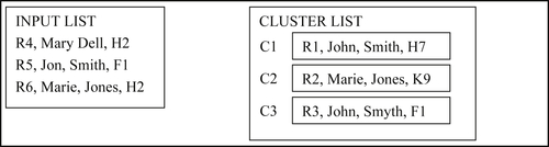
The first factor describes what is called a cluster (or a structure) projection. Figure 8.1 shows an example of an input reference R3 and a cluster of previously linked references R1 and R2. In this example, the pair-wise matching rule states that two references are classified as a match if they agree on first name and last name, or if they agree on employer identifier (“ID”).
The two most common types of projections are record-based projection and attribute-based projection (Zhou & Talburt, 2011c). In record-based projection, the incoming reference simply participates in pair-wise matching with each reference in Cluster C1. In other words, the answer to the question about how to select attribute values to use in the base rule is that the attribute values selected must come from the same reference in the cluster.
In the example of Figure 8.1, there are two previously processed references R1 and R2 that form Cluster C1 because they satisfied the base match rule by agreeing on the ID value. In the scenario shown, an input reference R3 comes into the system to be compared to Cluster C1. In a record-based projection model, there are two possible selections. The attribute values of R3 can be compared to the attribute values of R1 and R2. However, it is easy to see that neither of these would be classified as a matching pair. When R3 is compared to R1, the first names agree, but the last names and ID values disagree. When R3 is compared to R2, the last names agree, but the first names and ID values disagree. In record-based projection, the projections of the cluster correspond to the individual references in the cluster. In other words, a cluster comprising 10 references would produce 10 projections.
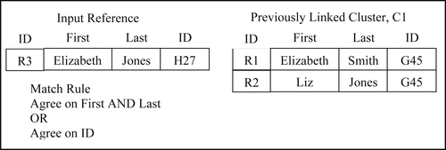
In this example, part of the answer to how many matches must succeed seems obvious. If the input reference does not match any of the references in the cluster, then the overall reference-to-cluster comparison should be classified as a no-match. On the other hand, if the input reference matches one or more of the references in the cluster, how many is enough to say that the reference should be part of the cluster? In general, the answer is that one is enough, i.e. if the input reference matches at least one of the projections from the cluster then the overall reference-to-cluster comparison is considered a match. The reason for this is the “principle of transitive closure” that will be discussed later. However, requiring only a single match is not universally true in all systems. In some cases, the requirement may be set higher – for example, that the input reference must match every projection from the cluster.
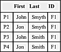
In an attribute-based projection, the attribute values used to compare to the input reference are not required to come from the same reference in the cluster. If an attribute-based projection is used in the example of Figure 8.1, the input reference R3 could be compared to four possible projections of the First, Last, and ID values in Cluster C1. These are shown in Table 8.1.
Note that projections P1 and P4 correspond to references R1 and R2, respectively. However, projections P2 and P3 do not correspond to actual references but are combinations of attributes taken from R1 and R2. In this case, the input reference R3 would match projection P3 according to the first condition of the base match rule, i.e. First and Last values agree.
The fact that R3 matches one of the attribute-projections of the cluster again brings up the question of how many projections should match in order to say that the reference matches the entire cluster. And again the answer is that in most systems matching one cluster projection is sufficient for the overall reference-to-cluster comparison to be considered a match.
The same logic for record-based and attribute-based projection can be extended to the more general case of cluster-to-cluster classification. Reference-to-cluster classification is just a special case of cluster-to-cluster classification, where one cluster comprises a single reference. In the general case, each projection from the first cluster is compared to each possible projection of the second cluster until, or if, enough pair-wise projections are classified as a match in order for the cluster-to-cluster classification to be considered a match.
Table 8.1
Attribute-based Projections of C1
| First | Last | ID | |
| P1 | Elizabeth | Smith | G45 |
| P2 | Liz | Smith | G45 |
| P3 | Elizabeth | Jones | G45 |
| P4 | Liz | Jones | G45 |
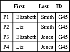
The number of attribute-based projections can grow dramatically. Just as a simple example, suppose that references have three identity attributes A1, A2, and A3. Also, suppose that cluster C1 contains three references and cluster C2 contains four references. A record-based cluster-to-cluster comparison would require at most 12 (3 times 4) reference-to-reference comparisons. On the other hand, in the worst-case scenario where all of the attribute values are unique within the cluster, then the number of distinct attribute-based projections from cluster C1 would be 27 (33) and from cluster C2 there would be 64 (43). Together these would yield 1,728 possible projection-to-projection comparisons. However, the actual number will typically be much smaller since the expectation is that references in the same cluster will share many of the same attribute values, and will not all be unique. In the example of Figure 8.1, Table 8.1 shows that even though a cluster of two references with three attributes could produce eight (23) attribute-based projections, there are actually only four projections of C1 because the attribute ID has only one value “G45”.
The Unique Reference Assumption and Transitive Closure
The next question is this: once the conditions are defined for classifying a cluster-to-cluster comparison as a match, what should happen to the clusters? Most often, the two clusters are merged into a single cluster, and all references in the merged cluster are given the same link value. Such an approach is in alignment with the Unique Reference Assumption that states “every reference is created to refer to one and only one real-world entity.”
Given this assumption, suppose that the system has determined that reference R1 is equivalent to R2, i.e. R1 and R2 refer to the same real-world entity E1. Suppose now a third reference R3 is determined equivalent to R2, i.e. R2 and R3 refer to the same real-world entity E2. Because R2 references both E1 and E2, it follows by the Unique Reference Assumption that E1 and E2 are the same entity, therefore R1, R2, and R3 are all equivalent because they all reference the same entity.
If a relationship has the property that “A relates to B” and “B relates to C” implies that “A relates to C,” then it is called a transitive relationship. The unique reference assumption provides the argument that reference equivalence is a transitive relationship among references. In other words, R1 is equivalent to R2, and R2 is equivalent to R3, implies that R1 is equivalent to R3. From an ER perspective that means that all three references R1, R2, and R3 should be linked together. Transitivity of reference equivalence also explains why in reference-to-cluster classification, even if an input reference matches only one reference (or attribute-projection) in a cluster, it is equivalent to all of them. The reference can be classified as a match for the entire cluster and can be merged into the cluster.
It often happens that an input reference can match two or more clusters. Even in this case, the same rule of transitive closure of reference equivalence is usually followed, and all of the clusters that match the input reference are merged together along with the input reference itself into a single cluster. A reference that matches and causes the merger of two or more references is sometimes called a glue record.
It is important to note that even though reference equivalence is transitive, matching itself is not transitive. If reference R1 matches reference R2, and R2 matches reference R3, it does not follow that R1 will match R3. For example, consider a simple match rule that says two strings match if they differ by at most one character. Then for this match rule it would be true that “ABC” matches “ADC”, and that “ADC” matches “ADE”, but it is not true that “ABC” matches “ADE”.
Selecting an Appropriate Algorithm
Once the cluster-to-cluster classification method has been decided, the next question is which ER algorithm should be used to systematically compare each input reference to previously processed references. The most desirable algorithm should have three characteristics:
1. It should find all possible matches. It should select and compare references in a way that whenever two reference match they will be compared, i.e. for a given base rule for pair matching and a cluster-to-cluster classification method, if a reference-to-reference match, or a reference-to-cluster match, or a cluster-to-cluster match is possible given the references in the input source, then the algorithm will systematically select the references and clusters in such a way that these comparisons will be made.
2. It should be efficient. At the same time it does not lose matches, it should try minimizing the number of attempted comparisons among references and clusters to find those matches, i.e. it should avoid spending time on comparisons that will not result in a match. For example, one way to find all possible matches is to use the “brute force” method that exhaustively compares every cluster to every other cluster. However, brute force is not efficient.
3. It should be sequence neutral, i.e. the clusters created at the final step should be the same regardless of the order that the input references are processed by the algorithm. This property is really a corollary of the first characteristic provided the algorithm obeys transitive closure.
The degree to which possible matches are found (Characteristic 1) is called the recall of the algorithm. If R is a set of N references, and P is the set of all distinct, unordered pairs of references from R, then the number of pairs in P is given by
![]()
For a given match rule, let M represent the pairs of references in P that would actually match by the rule. In general the size of M will be much smaller than P. Given an algorithm A for selecting pairs in P for matching, let pairs found by A that actually match be represented by F. Then the match recall of A is given by
![]()
It is easy to guarantee that Recall(A) is 100% by having the algorithm compare every pair of references in P. However, according to the first formula the number of pairs in P grows with the square of N, the number of references in R. Even for fast processing systems using an ER algorithm that makes every possible comparison between references, time performance will be unacceptable. In addition, ER does not easily lend itself to parallel and distributed processing.
For practical purposes the ER algorithm A must select only some subset of P as candidates for matching. Let C represent the set of pairs in P that are selected by the algorithm A. Then the efficiency of the algorithm (Characteristic 2) called its match precision is given by
![]()
The match precision of A measures the ratio of matching pairs found by A to the total number of pairs compared by A.
As noted earlier, the recall of an algorithm (Characteristic 1) and its ability to be sequence neutral (Characteristic 3) are related to each other. If the algorithm is sensitive to the order in which the references are processed, it may miss some matches that it might have found if the references were processed in a different order. In addition, there is a dependency upon the choice of cluster projection used for cluster-to-cluster matching. An algorithm that has all three characteristics when record-based projection is used may fail in some characteristics if attribute-based projection is used.
To help illustrate these concepts, a series of examples will be shown. For each example, the input and base rule for matching pairs of references will be the same. Table 8.2 shows the input references used in the examples.
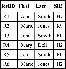
Similar to the previous example concerning cluster projections, each reference has four attributes: a record identifier (RefID), a first name value (First), a last name value (Last), and a school identifier (SID).
In addition, all of the examples will use the same base rule for pair matching:
Base (Boolean) Rule for matching pairs of references
(First values agree) AND (Last values agree)
OR
(SID values agree)
The One-Pass Algorithm
The One-Pass Algorithm is a simple algorithm that is more efficient than brute force yet still able to find all possible matches for certain cluster-to-cluster classification schemes. Its name comes from the fact that each input reference is only processed one time, i.e. one pass through the input references.
The algorithm starts with a list of input references and an empty output list of clusters. Each input reference is processed in order by comparing it to all of the clusters in the output list. If it matches one or more clusters in the output list, then all of the clusters that it matches are merged together, including the input reference itself, to form a new cluster. In the case where the input reference does not match any one of the clusters in the output list, it forms a new single-reference cluster appended to the end of the cluster list. This continues until all of the input references have been processed.
Configuration Choices for Example 8.1:
1. Base rule for matching reference pairs: Boolean rule (First Agree) AND (Last Agree) OR (SID Agree)
2. Cluster projection: Record-Based
3. Cluster-to-Cluster Match Rule: Single Match
4. Transitive Closure: Yes
5. ER Algorithm: One-Pass
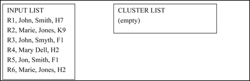
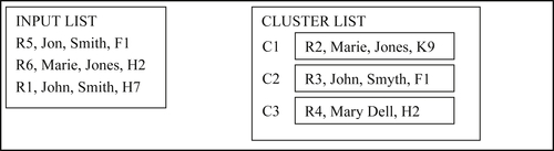
Figure 8.2 Starting conditions for Example 8.1.
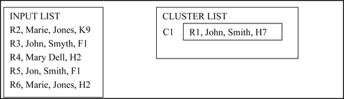
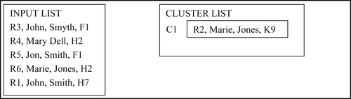
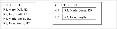
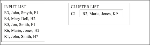
The starting conditions for the example input are shown in Figure 8.2. When the first input reference R1 is processed, there are no clusters to compare it with, and therefore it is simply made into the single-reference cluster C1 as the first item in the Cluster List, as shown in Figure 8.3.
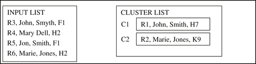
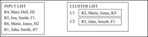
In the next step, Reference R2 is processed. In this case, there is only one reference-to-cluster comparison of R2-to-C1. The cluster projection for this example is record-based projection. This means that C1 only projects one set of values to be compared to R2, namely the values that comprise R1. Because the R1 values do not march the R2 values according to the base rule, R2 creates a new cluster C2 as shown in Figure 8.4.
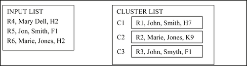
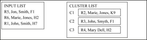
In the third step, Reference R3 is processed. Now there are two reference-to-cluster comparisons of R3-to-C1 and R3-to-C2. Again, C1 only projects the R1 values and these do not match R3 by the base rule. C2 only projects the R2 values and these do not match R3 either. Therefore, R3 creates a new cluster C3, as shown in Figure 8.5.
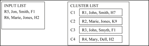
In the fourth step, Reference R4 is processed and there are three reference-to-cluster comparisons of R4-to-C1, R4-to-C2, and R4-to-C3. Each cluster only projects one set of values from the single reference in the cluster. The values of R4 do not match any of these projections, and therefore, it creates a new cluster C4 as shown in Figure 8.6.
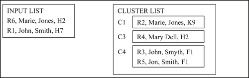
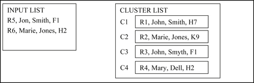
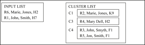
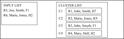
In the fifth step, Reference R5 is processed and there are now four reference-to-cluster comparisons of R5-to-C1, R5-to-C2, R5-to-C3, and R5-to-C4. Again, each cluster only projects one set of values from the single reference in each cluster. However, in this step the SID value in R5 matches the SID value projected from C3 according to the second part of the base rule. Consequently, R5 is merged with Cluster C3 to form a new Cluster C5 as shown in Figure 8.7.
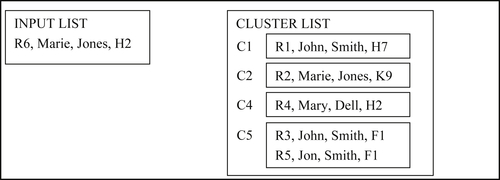
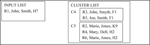
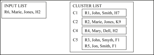
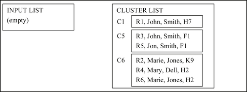
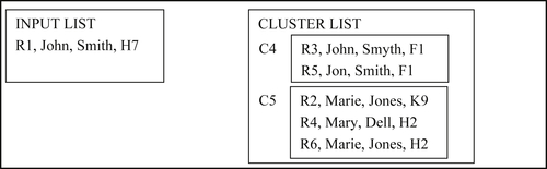
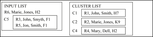
In the sixth and final step, Reference R6 is processed. There are four reference-to-cluster comparisons of R6-to-C1, R6-to-C2, R6-to-C4, and R6-to-C5. Clusters C1, C2, and C4 only project one set of values from the single reference in the cluster. By record-based project, C5 projects two sets of values, one set of value from R3 and one set values from R5. At this step, R6 matches name values projected from C2 according to the first part of the base rule, and R6 also matches the SID value projected from C4 according to the second part of the base rule. In this case, R6 acts as a glue record causing R6, C2, and C4 to merge into a single cluster C6 as shown in Figure 8.8.
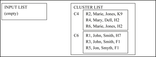
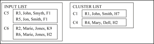
The final result is that the six input references are linked together into three clusters, cluster C1 comprising reference R1, cluster C5 comprising references R3 and R5, and cluster C6 comprising references R2, R4, and R6. However, this result is dependent upon all of the configuration choices stated at the beginning. Change any of these parameters and the clustering results for the same input dataset may be different, as will be shown in later examples.
The configuration choices for Example 8.2 are the same as for Example 8.1, the only difference being that the input has been reordered so that reference R1 now appears at the end of the input list instead of at the beginning as shown in Figure 8.9.
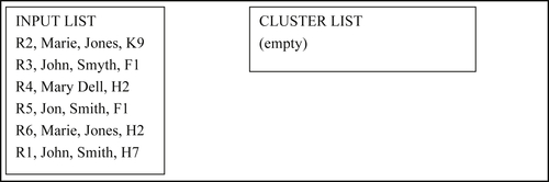
Figure 8.9 Starting conditions for Example 8.2.
The first input reference R2 forms the single-reference cluster C1 as shown in Figure 8.10.
In the next step, the second reference R3 forms a single-reference cluster C2 as shown in Figure 8.11.
In the third step, Reference R4 is processed and forms the single-reference cluster C3 as shown in Figure 8.12.
In the fourth step, Reference R5 matches cluster C2 and merges to form cluster C4 as shown in Figure 8.13.
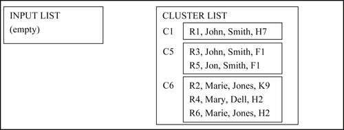
In the fifth step, Reference R6 matches both C1 and C3 to form the new cluster C5 as shown in Figure 8.14.
In the sixth and final step, Reference R1 is processed and does not match any of the projections from clusters C4 and C5, and forms the new single-reference cluster C6 as shown in Figure 8.15.
The final result is that the six input references are linked together into three clusters, cluster C4 comprising references R2, R4, and R6, cluster C5 comprising references R3 and R5, and cluster C6 comprising reference R1. The important point here is that even though the cluster labels are different, the clustering is the same as in Example 8.1 as shown in Figure 8.8, i.e. the order of processing did not affect the ER results, the same references were clustered together. Although this does not constitute a proof, it is true that One-Pass is sequence neutral when record-based projection is used for cluster-to-cluster matching. The next two examples show that One-Pass is not always sequence neutral when attribute-based projection is used.
Configuration choices for Example 8.3:
1. Base rule for matching reference pairs: Boolean rule (First Agree) AND (Last Agree) OR (SID Agree)
2. Cluster projection: Attribute-based
3. Cluster-to-Cluster Match Rule: Single Match
4. Transitive Closure: Yes
5. ER Algorithm: One-Pass
The first part proceeds much the same as in Example 8.1.
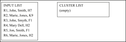
Figure 8.16 Starting conditions for Example 8.3
The starting conditions for the example input are shown in Figure 8.16. When the first input reference R1 is processed, it forms the single-reference cluster C1 as shown in Figure 8.17.
In the next step, reference R2 creates a new cluster C2 as shown in Figure 8.18.
In the third step, reference R3 creates a new cluster C3 as shown in Figure 8.19.
In the fourth step, Reference R4 creates a new cluster C4 as shown in Figure 8.20.
In the fifth step, Reference R5 matches C3 and a new Cluster C5 is formed by the merger as shown in Figure 8.21.
In the sixth and final step, Reference R6 is processed. Just as before, there are four reference-to-cluster comparisons of R6-to-C1, R6-to-C2, R6-to-C4, and R6-to-C5. Even though this example uses attribute-based projection, Clusters C1, C2, and C4 only project one set of values from the single reference in the cluster. However, in the R6-to-C5 comparison, C5 produces three projections that are shown in Table 8.3.
At this step, R6 still matches the name values projected from C2, and the SID value projected from C4. The fact that C5 produces two additional projections does not result in any additional matches for this step. Therefore, the result for Example 8.3 is the same as for Examples 8.1 and 8.2 as shown here in Figure 8.22.
The configuration choices for Example 8.4 are the same as for Example 8.3; the only difference is the input has been reordered so reference R1 now appears at the end of the input list instead of at the beginning as shown in Figure 8.23. The purpose of this example is to show the One-Pass algorithm is not sequence neutral when used in conjunction with attribute-based projection.
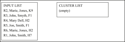
Figure 8.23 Starting conditions for Example 8.4.
The first input reference R2 forms the single-reference cluster C1 as shown in Figure 8.24.
In the next step, the second reference R3 forms a single-reference cluster C2 as shown in Figure 8.25.
In the third step, Reference R4 is processed and forms the single-reference cluster C3 as shown in Figure 8.26.
In the fourth step, Reference R5 matches cluster C2 and merges to form cluster C4 as shown in Figure 8.27.
In the fifth step, Reference R6 matches both C1 and C3 to form the new cluster C5 as shown in Figure 8.28.
In the sixth and final step, something different happens. Cluster C4 now produces four projections, the same projections that were produced from Cluster C5 in the previous example and shown in Table 8.3. In particular, R1 matches projection P3. Therefore, R1 is merged into C4 to produce a new cluster C6 as shown in Figure 8.29.
The final result is that two clusters of three references are fundamentally different than the results in Examples 8.1, 8.2 and 8.3. In particular, this example shows that the One-Pass algorithm is not always sequence neutral when attribute-based projection is used. When the configuration choice is attribute-based projection, then an ER algorithm stronger than the One-Pass algorithm is required.
The R-Swoosh Algorithm
The R-Swoosh ER algorithm was developed at the Stanford InfoLab oun, Garcia-Molina, Su, & Widom, 2005). The R-Swoosh algorithm is part of a larger body of ER research called the Stanford Entity Resolution Framework (SERF). As described in Chapter 7, the SERF model describes entity resolution in terms of abstract match and merge functions, and shows the conditions that must hold for these functions so the ER process will always arrive at a finite, unique, and sequence-neutral outcome. An important component of SERF is the Swoosh family of ER algorithms, of which R-Swoosh is the most basic.
The R-Swoosh algorithm is similar to the One-Pass in that it starts with a list of input references and an empty output list of clusters. The primary difference is that clusters from the output list are sometimes pushed back into the input list for reprocessing. Here is how that happens. When an item on the input list is selected for processing, it is compared in order to each cluster in the output list. If a comparison results in a match, the input item is removed from the input list and merged with the matching cluster. The new merged cluster is removed from the output list and appended to the end of the input list. The algorithm continues by processing the next item in the input list until the input list is empty. In the case where an input item does not match any of the clusters in the output list, it forms a new single-reference cluster that is appended to the end of the cluster list the same as in the One-Pass algorithm. The algorithm continues until all of the input items have been processed.
Configuration choices for Example 8.5:
1. Base rule for matching reference pairs: Boolean rule (First Agree) AND (Last Agree) OR (SID Agree)
2. Cluster projection: Attribute-Based
3. Cluster-to-Cluster Match Rule: Single Match
4. Transitive Closure: Yes
5. ER Algorithm: R-Swoosh
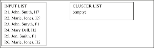
Figure 8.30 Starting conditions for Example 8.5.
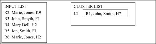
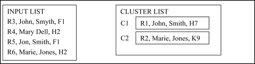
Because there are no matches among the first four references, these all create single-reference clusters as shown in Figure 8.31.
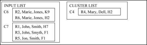
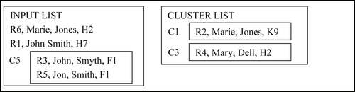
Up to this point, R-Swoosh behaves the same as One-Pass. However, in the fifth step there is a difference. In the R5-to-C1 and R5-to-C2 comparisons there is no match, but R5-to-C3 is a match on SID. In the R-Swoosh algorithm R5 is merged into C3 to form a new cluster C5. R5 and C3 are removed from the input list and output list, respectively, and the new cluster C5 is appended to the end of the input list for reprocessing as shown in Figure 8.32.
Unlike the previous examples, the sixth step is no longer the final step because there are now two items still in the input list. When reference R6 is processed, the first match it finds is to C2. This stops the comparisons, and R6 is merged with Cluster C2. The new merged cluster C6 is appended to the input list as shown in Figure 8.33.
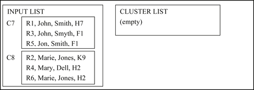
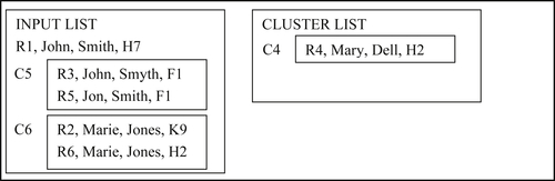
In the seventh step, cluster C5 is compared to C1. By attribute projection, cluster C5 will produce four projections, the same as those shown in Table 8.3, and in fact, project P3 of Table 8.3 is a match to the single projection of C1. Consequently, clusters C5 and C1 are merged into a new cluster C7 that is appended to the input list as shown in Figure 8.34.
In the eighth step, cluster C6 is compared to C4. Because these two clusters match, they are merged into a new cluster C8 that is an appended input list as shown in Figure 8.35. Although the cluster list is empty, the algorithm does not stop until the input list is empty.
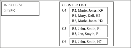
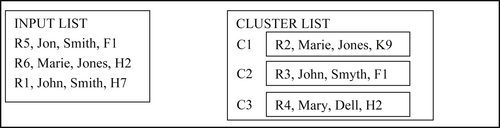
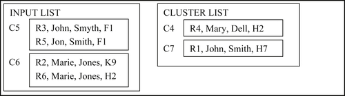
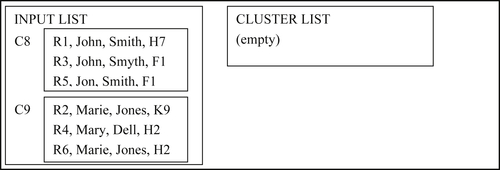
In the ninth step, cluster C7 is simply moved to the empty cluster list. In the tenth and last step, cluster C8 is compared to cluster C7. Because these two clusters do not match, cluster C8 is also moved to the end of the cluster list as shown in Figure 8.36. This also results in an empty input list and so the algorithm ends at the tenth step.

The configuration for this example is exactly the same as for the previous Example 8.5 except that the input list has been reordered so that reference R1 is placed at the end of the input list instead of at the beginning, as shown in Figure 8.37.
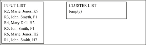
Figure 8.37 Starting conditions for Example 8.6.
Because there are no matches among the first three references, these all create single-reference clusters as shown in Figure 8.38.
In the fourth step, reference R5 matches cluster C2. Following the R-Swoosh algorithm, R5 and C2 are merged to create new cluster C4 that is appended to the input list as shown in Figure 8.39.
In the next step, reference R6 is found to match cluster C1. R6 and C1 are merged to form a new cluster C6 that is appended to the input list, as shown in Figure 8.40.
In the sixth step, reference R1 is compared to cluster C4 and found not to be a match. Reference R1 forms a new cluster C7 that is appended to the cluster list as shown in Figure 8.41.
In the seventh step, cluster C5 is first compared to C4 and found not to be a match. However, through attribute-based projection, cluster C5 is a name match to cluster C7 as in the previous Example 8.5. Clusters C5 and C7 are merged to form a new cluster C8 that is an appended input list as shown in Figure 8.42.

In the eighth step, cluster C6 matches and merges with C4 to form cluster C9 that is appended to the input list as shown in Figure 8.43.
At this point, the algorithm is essentially complete. In the ninth step, cluster C8 is moved to the cluster list, and in the tenth step, cluster C9 is compared to cluster C8, but does not match. Therefore, cluster C9 is appended to the cluster list and the algorithm ends with an empty input list as shown in Figure 8.44.
Although these examples do not establish a proof, at least Examples 8.5 and 8.6 show that the R-Swoosh algorithm produces the same results for attribute-based projection when presented with the differently ordered lists that caused the One-Pass to give different results when using attribute-based projection as demonstrated in Examples 8.3 and 8.4.
Concluding Remarks
The previous examples have shown that some combinations of ER design choices will lead to undesirable results. Examples 8.1 and 8.2 show the combination of the One-Pass algorithm with record-based cluster matching produces the same clustering results for two different orderings of the input list. It is not difficult to show this combination is actually sequence neutral, i.e. will give the same clustering results for any ordering of the input list.
Table 8.4
Summary of ER Design Scenarios for Same Input and Base Rule
| Scenario | Algorithm | Cluster Matching | Sequence Neutral | Cluster Results |
| 1 | One-Pass | Record-based | Yes | N Clusters |
| 2 | R-Swoosh | Attribute-based | Yes | M Clusters where M ≤ N |
| 3 | One-Pass | Attribute-based | No | Varies by Order of Input |
| 4 | R-Swoosh | Record-based | Yes | N Clusters, but Inefficient |
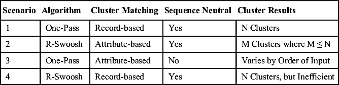
However, Examples 8.3 and 8.4 demonstrate that the combination of the One-Pass algorithm with attribute-based projection cluster matching is not sequence neutral. They show that different orderings can produce different clustering results. Examples 8.5 and 8.6 show that the combination of the R-Swoosh algorithm with attribute-based cluster matching gives the same clustering results for both orderings. Benjelloun et al. (2009) have shown that this will always be the case, i.e. the combination of R-Swoosh and attribute-based cluster matching will be sequence neutral.
It is also worthwhile to note that because an attribute-based projection can produce more pair-wise attribute value combinations to test than a record-based projection, then it follows that using the R-Swoosh algorithm with attribute-based projection will often find more matches than the One-Pass algorithm using record-based projection. From this it also follows that the total number of clusters produced by R-Swoosh and attribute-based projection will always be less than or equal to the total number of clusters produced by One-Pass and record-based projection as shown in Examples 8.1 and 8.5. Acting on the same input list, One-Pass using record-based projection produced three clusters in Example 8.1 while R-Swoosh using attributed-based projection produced two clusters in Example 8.5. The reason is that with transitive closure, more matches yields a higher likelihood of producing a glue record that will merge two clusters. In other words, more matching means fewer clusters.
A summary of these design combinations is shown in Table 8.4. Note that even though Scenario 4 is a valid sequence neutral combination, it would be better to use Scenario 1 instead. Using R-Swoosh with record-based matching is inefficient because the extra comparisons are not necessary to achieve the correct result. One-Pass will give the same clustering result with fewer comparisons.
..................Content has been hidden....................
You can't read the all page of ebook, please click here login for view all page.