This chapter describes how a distributed processing environment such as Hadoop Map/Reduce can be used to support the CSRUD Life Cycle for Big Data. The examples shown in this chapter use the match key blocking described in Chapter 9 as a data partitioning strategy to perform ER on large datasets. The chapter includes an algorithm for finding the transitive closure of multiple match keys in a distributed processing environment using an iterative algorithm that minimizes the amount of local memory required for each processor. It also outlines a structure for an identity knowledge base in a distributed key-value data store, and describes strategies and distributed processing workflows for capture and update phases of the CSRUD life cycle using both record-based and attribute-based cluster-to-cluster structure projections.
Keywords
Big Data; Hadoop Map/Reduce; Transitive Closure; Graph Component
Large-Scale ER for MDM
As noted earlier, in the world of ER small data can quickly become big data because ER is fundamentally an O(n2) problem. Match key blocking, as discussed in Chapter 8, is one of the primary strategies for addressing the problem of large-scale ER (Bianco, Galante, & Heuser, 2011; Kirsten et al., 2010; Yancey, 2007). This is because properly aligned match key blocking will partition the set of input references into disjoint subsets that can be resolved independently of one another. This makes match key blocking ideal for distributed processing applications such as Hadoop Map/Reduce that do not support or require processor-to-processor communication. However, this approach will only work as long each block is small enough to fit into the memory of any single processor.
The Hadoop Map/Reduce is a processing layer that sits on top of the Hadoop File System (HDFS). In the Hadoop architecture, a mapper function outputs key-value pairs. The system then brings together all of the key-value pairs into blocks that share the same key. These blocks are then processed by reducer functions. This paradigm fits nicely with match key blocking in which the key of the key-value pair is the match key, and the value of the key-value pair is the reference.
Large-Scale ER with Single Match Key Blocking
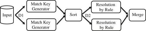
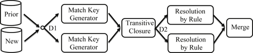
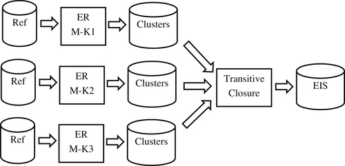
Suppose for a base ER rule there is a single, properly aligned index generator. Alignment of the index generator with the match rule implies all pairs of references that match by one of the rules also generate the same index value. Therefore, from an entity resolution standpoint, this means all of the matches that can be found by the match rule are going to be found between references within the same block. By the assumption of alignment, references from different match key blocks should not match. Consequently in the case of a single index generator, the complete resolution of a dataset can be accomplished in a relatively simple, two-step process as shown in Figure 10.1.
The first step is the generation of the match key values. At this first step, the partitioning and distribution D1 of the input references to different processors is arbitrary and can simply be based on uniformly sized groupings of references. This is because the match key value produced by a match key generator only depends upon the values of the identity attributes in each reference, and there are no dependencies on other references. In the Hadoop Map/Reduce framework, algorithms such as match key generation that operate independently on individual records are usually run in a map step. The output of a map step is always a key-value pair. In this case the key of the key-value pair is the generated match key, and the value of the key-value pair is the reference that generated the match key.
Figure 10.1 Distributed workflow based on single index generator.
After each block of input references has been processed by the match key generator running at each of the nodes, each reference will produce a single match key. These match key-reference pairs are then merged and sorted into match key value order. In the Hadoop Map/Reduce framework, sorting by key value is performed by a shuffle step that follows the map step and precedes the reduce step. Unless otherwise specified, the shuffle sorts the mapper output in key value order by default.
After the references are sorted into match key order, Hadoop automatically creates key-blocks. Each key-block comprises all of the key-value pairs that share the same key value. In this case, it will be blocks of references where all of the references in the same block share the same match key value.
In the reduce step, the key-blocks are distributed to different processors where the final resolution of blocks into clusters takes place. Again, this fits well with the Hadoop map/reduce framework that guarantees all of the records in a key-block are processed together on the same processor. One processor could be given multiple blocks, but the reducer function of Hadoop assures blocks are not split across processors.
Once a block of key-value pairs is sent to a processor, it can be processed by an ER algorithm and base match rule to link the references into clusters. Consequently, in a Hadoop framework the ER process itself works best in a reduce step. Taking again the example of blocking by postal code, the key of the key-value pair would be the postal code and the value of the key-value pair would be the actual reference. In this way, all references with the same postal code would be sent to the same processor. The reduce step guarantees blocks with the same postal code will be sent to the same processor provided the postal code block does not exceed the capacity of a single processor. Typically key blocks will be smaller than the single process capacity, allowing the system to send several key blocks to the same processor. The reducer provides an iterator function that allows the code resident on the processor to access each key-value pair in the key-block sequentially. In the final reduce step each postal code block becomes the input to an ER algorithm that will further refine the block into clusters according to the matching rules of the ER process.
Decoding Key-Value Pairs
From the viewpoint of a map/reduce process, all records only have two fields, a key field and a value field separated by a special character, by default a tab character. Although the keys and values can be typed, they are usually handled as text (character strings). Therefore, it is the responsibility of the application developer to interpret the value portion of the key-value pairs as a reference comprising several attribute-value pairs, i.e. subvalues of a value string. The subvalues representing the attribute values of the reference can be encoded into the overall string representing the single-value of the key-value pair in many different ways. For example, the encoding can be comma-separated values (CSV) or even traditional fixed-field width record format. Talburt and Nelson (2009) have developed a Compressed Document Set Architecture (CoDoSA) that uses short metadata tags in the string to separate and identify the subvalues encoded into an overall string. CoDoSA encoding resembles a lightweight XML document. CoDoSA is the standard for encoding references in the EIS of the OYSTER Open Source Entity Resolution system (Talburt & Zhou, 2012, 2013). An example of an OYSTER EIS using CoDoSA reference encoding is shown in Figure 1.3 of Chapter 1.
In the case of a single index as shown in Figure 10.1, both distributions D1 and D2 actually create true partitions of the datasets A and B, respectively – i.e. the distributed segments are nonoverlapping. D1 can partition the input by simply counting off equal size blocks of references. D2 partitions the match key-value pairs because each reference has only one match key value; thus the match key blocks cannot overlap.
The Transitive Closure Problem
However, there is a problem associated with the process described in Figure 10.1. The problem is that, in most large-scale entity resolution applications, a single match key is not sufficient to bring together all of the references that should be compared. Data quality problems such as typographical errors in attribute values, missing values, and inconsistent representation of the values will require the use of more than one match key in order to obtain good resolution results with a reasonable amount of comparison reduction. This problem is particularly acute when the base match rule is a scoring rule. As described in Chapter 9 in the section titled “Match Key Blocking for Scoring Rules,” a simple scoring rule comparing only a few identity attributes may need support from dozens of match key generators.
When each input reference can potentially create more than one match key, the processing method outlined in Figure 10.1 will not always lead to the correct resolution of the references in the input. The reason is the requirement for transitive closure of an ER process. Transitive closure states if a reference R1 is linked to a reference R2, and reference R2 is linked to a reference R3, then reference R1 should be linked to reference R3.
To see how having multiple match key generators disrupts the process described in Figure 10.1, suppose there are three distinct references R1, R2, and R3, and two match key generators Gen1 and Gen2. Table 10.1 shows the results of applying the two match key generators to the three references.
Because each reference generates two keys, the final result is a set of six match key-value pairs. These pairs in sorted order by match value are shown in Table 10.2.
The four distinct key values partition the key-value pairs into four blocks. The first block has two key-value pairs that share the match key value of K1. The second block formed by the match key K2 has only a single key-value pair. The third block has two key-value pairs formed by the match key K3, and finally the last block is a single key-value pair formed by the match key K4.
The first observation is that, even though the keys partition the key-value pairs, they do not partition the underlying set of references. The references in the K1 block overlap with the references in the K2 and K3 blocks at references R1 and R2, respectively. Any reference that generates two or more distinct match keys will be duplicated in each of the blocks for those match keys.
Now suppose in a distributed processor scheme the K1 and K2 blocks are sent to processor P1, and the K3 and K4 blocks are sent to another processor P2. Further suppose when the ER process running on P1 processes the K1 block, it finds that R1 and R2 are matching references and links them together. Similarly suppose when the ER process running on P2 processes the K3 block, it finds that R2 and R3 are matching references and links them together.
Table 10.1
Match Key Values
Reference
Gen1
Gen2
R1
K1
K2
R2
K1
K3
R3
K4
K3
Table 10.2
Pairs Sorted by Match Key
Key
Value
K1
R1
K1
R2
K2
R1
K3
R2
K3
R3
K4
R3
The combined output of this process comprises four clusters: {R1, R2}, {R1}, {R2, R3}, and {R4}. However, this result is not consistent with the principles of ER. The final output of an ER process should be a true partition of the original input, i.e. each reference should be in one, and only one, cluster, and the clusters should not overlap with each other. Clearly when references can generate multiple match keys, the simple process shown in Figure 10.1 no longer works.
The approach to solving the multiple-index problem depends upon whether the ER processes are using record-based resolution or attribute-based resolution as described in Chapter 8. The solution for multiple match keys when the ER system is using record-based projection is simpler than one using attributed-based projection, so it will be discussed first.
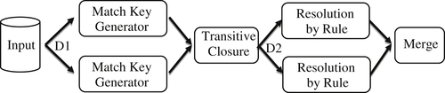
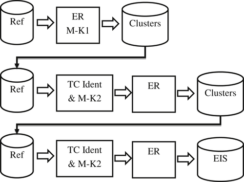
The workflow for multiple match key resolution as shown in Figure 10.2 begins in the same way as the process outlined in Figure 10.1 for a single index workflow. The problem is that simply sorting and distributing by match key blocks is no longer adequate. As discussed in the previous example, simply sorting to create distribution D2 may cause the final result to contain clusters of overlapping references.
One solution to the problem shown here is to replace the sort process with a transitive closure process where the closure is with respect to shared match key values. This can most easily be understood by looking at the references and relationships in the form of a graph.
Transitive Closure as a Graph Problem
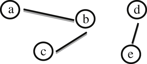
In graph theory an undirected graph is simply a set N of nodes and a set of E of edges, where E is a subset of P(N), the set of all subsets of N that contain two elements. As a simple example consider, N = {a, b, c, d, e} and E = {{a, b}, {b, c}, {d, e}}. N and E form an undirected graph of five nodes and three edges depicted in Figure 10.3.
A connected component of a graph is a maximal subset of nodes in the graph having the property for any two nodes in the subset, there exists a path of edges that connects them together. In Figure 10.3, it is easy to see the graph has two connected components {a, b, c} and {d, e}. Even though node “a” and node “c” do not share an edge, there is a path from “a” to “b” and from “b” to “c” that connects them. It will also be true the connected components of a graph form a partition of the nodes, i.e. every node in the graph is in one, and only one, component.
Figure 10.2 Distributed workflow for multiple match keys.
Figure 10.3 Undirected graph of N and E.
A connected component represents the transitive closure of the nodes in the component with respect to connections between nodes. The standard algorithm for finding the components of a graph uses this principle (Sedgewick & Wayne, 2011). It starts by selecting any node in the graph, and then finds all of the nodes connected to it. Next, all of the nodes connected to these nodes are found, then the nodes connected to these, and so on until no new connections can be made. The set of nodes found in this way comprises the first component of the graphs. The next step is to select any node not in the first component and form its component in the same way as the first. This process stops when there are no more nodes outside of the components that have already been found.
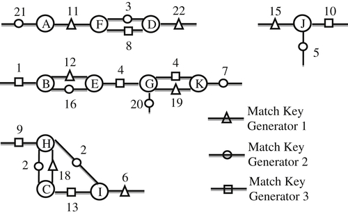
References and Match Keys as a Graph
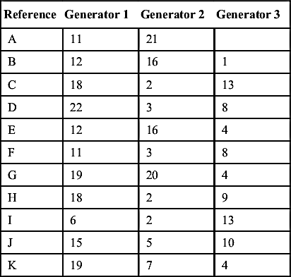
References and their match keys can also be given a graphical interpretation. Consider the following example of 11 references {A, B, C, D, E, F, G, H, I, J, K} and 3 index generators. For simplicity, the match key values in Table 10.3 are given as integer values. By the design of the match key generators, the values produced by one generator will be different from the set of values produced by a different generator. However, in general there will be duplication among the values produced by the same generator.
The references and match keys in Table 10.3 can be interpreted as a graph in which the references are the nodes of the graph and match keys shared by two references form an edge in the graphs. Figure 10.4 shows the graph interpretation of Table 10.3.
One notable difference between the match key graph in Figure 10.4 and the graph in Figure 10.3 is the match key graph is noisy. The noise is created by the fact that some references may generate unique keys not shared with any other reference, e.g. keys 21 and 22. A unique match key does not form an edge in the graph. Another source of noise is that some references share more than one match key, e.g. nodes F and D.
Although this noise makes the graph in Figure 10.4 look somewhat different from the graph in Figure 10.3, they still have the same essential features. Two references are connected if and only if they share at least one match key between them. It is also much easier to see the connected components of the references in the graph representation in Figure 10.4 than by inspecting Table 10.3. It is apparent the graph in Figure 10.4 has four connected components {A, D, F}, {J}, {B, E, G, K}, and {C, H, I}.
An Iterative, Nonrecursive Algorithm for Transitive Closure
The standard algorithm for finding the connected components of a graph is a breadth-first search algorithm that uses recursion (Sedgewick & Wayne, 2011). Although elegant, it has a limiting feature when working with Big Data. The standard recursive algorithm for transitive closure needs to have access to all the node and edge information in one memory space to work efficiently. In other words, the algorithm assumes it can directly access any part of the graph at any given point in the algorithm. For very large datasets this may not be practical or even possible.
Distributed processing using the Hadoop framework works best when it is operating on large key-value sets by successively performing record-level operations (mapper functions) followed by operations on key-values blocks (reducer functions). To better fit the processing paradigm, the authors have developed an iterative algorithm for finding the connected components of a match key graph like the one shown in Figure 10.4. The purpose of the algorithm is to perform the transitive closure of a graph through the iterative, sequential processing of a large set of key-value pairs without the need to create large, in-memory data structures.
The context and notation for the pseudo-code of this algorithm is that R represents a set of references, and G represents a set of N match key generators. If r is a reference in R, then r1, r2, r3, …, rN represent the key values generated by each of the index generators acting on r (some values may be null). The algorithm has three parts: an initial bootstrap phase, an iteration phase, and a final deduplication phase. Here is a general description of each phase and the key-value pairs they use.
• Bootstrap: In the bootstrap phase, the key of the key-value pair is a match key and the value of key-value pair is the reference. Each reference can generate up to N key-value pairs, one key-value pair for each non-null match key generated by the reference. In the bootstrap, the key value pairs are sorted by match key to find the connected pairs of references. The output of the bootstrap phase is a list where each item in the list is a set of reference identifiers of the references connected to each other by a shared match key value.
• Starting with the bootstrap phase, and in each following step, the items in the output list are sets of record identifiers. These sets of record identifiers are the proto-components of the graph, i.e. components in formation. At the bootstrap these proto-components are usually singleton sets or pairs of identifiers. The algorithm takes a bottom-up approach by first finding connected pairs of references in the bootstrap phase, then finding overlapping pairs in the first iteration phase to form triples, then quadruples in the next iteration, and so on. At the end of the bootstrap phase the match key values and the actual contents of the reference are discarded. Only reference identifiers are carried forward into the iteration phase. After the match keys have been generated, the attribute-value pairs of the reference are not needed for the actual transitive closure process and can be discarded for storage efficiency. At the end of the transitive closure process, the actual reference value can be recovered for use in the ER process by performing a simple join of the reference identifiers with the original input.
• Iteration: Each iteration phase starts with a list of proto-components. In the case of the first iteration, it is the list of proto-components from the bootstrap. In other iterations it is the list of proto-components output from the previous iteration. Each iteration begins by taking each proto-component produced in the previous step and expanding it into a set of key-value pairs where the key is a single reference identifier taken from the proto-component and the value is the entire proto-component. This means that if a proto-component contains N reference identifiers, then it forms N key-value pairs, one for each reference identifier in the proto-component. For example, if the proto-component comprises three reference identifiers {R1, R2, R3}, then it forms three key value pairs of (R1, {R1, R2, R3}), (R2, {R1, R2, R3}), and (R3, {R1, R2, R3}). After the expansion, the key-value pairs are sorted by key value. After the key-value pairs are sorted, all of the proto-components with the same key block are merged (set union) to produce a new proto-component. The new list of proto-components becomes the input for the next iteration. The iteration continues until no new proto-components are created at the merge step, i.e. the proto-components cease to grow in size as a result of the merging of all of the proto-components in the same key-value block.
• Deduplication: Due to the nature of the algorithm and the noise inherent in the match key graph, the same component may appear in different positions in the list. The final phase is to deduplicate the final list of components into a set of unique connected components. This is done by creating key-value pairs where the key value is the first reference identifier in the final component, and the value of the key-value pair is the entire component. After these key-value pairs are sorted by key value, only the first component in each key-value block is kept. This is because during the iteration phase, the reference identifiers are maintained in the proto-component sets in sorted order. Therefore, if two components agree on the first reference identifier, then they are the same component.
Bootstrap Phase: Initial Closure by Match Key Values
Let kList be a list of items where each item has two attributes. The first attribute is a non-null, match key value for a reference. The second attribute is the identifier (RefID) of the reference; kList should have one record for each possible combination of a reference r in R and a non-null match key value produced by one of the index generators in G acting on r. If kItem represents an item in kList, then kItem.key represents the value of the first attribute (match key value), and kItem.rid represents the value of the second attribute (RefID).
Let sList represent another list where each list item has two attributes; for sList the first attribute is an integer value and the second attribute is a set of RefIDs. If sItem represents an item of sList then sItem.int is the integer value and sItem.refSet is the list of RefIDs.
Bootstrap Start
Sort kList primary by key and secondary by RefID.
\ Write proto-components to sList by processing kList sequentially
1 → compNbr
kList.getNextItem() → kItem
kItem.rid → prevRid
kItem.idx → prevIdx
Declare compSet a Set of RefID
Ø → compSet
Ø → sList
While(More items in kList)
If((kItem.rid == prevRid) OR (kItem.idx) == prevIdx))
Then
compSet.insert(kItem.rid)
Else
compNbr → sItem.int
compSet → sItem.refSet
sList.append(sItem)
compNbr + 1 → compNbr
kItem.rid → compSet
kList.rid → prevRid
kList.idx → prevIdx
K.readNextRecord()→ kRec
End of While Loop
compNbr → sItem.int
compSet → sItem.refSet
sList.append(sItem)
Iteration Phase: Successive Closure by Reference Identifier
Let sList be the same list of items produced in the bootstrap phase, and let tList represent a list of items where the first attribute is a single RefID, and the second attribute is a Set of RefIDs.
\ This is an iterative process, stops when changeCnt is zero
1 → changeCnt
Ø → tList
While(changeCnt>0)
// Expand sList into tList
While(More items in sList)
sList.readNextItem()→ sItem
(sList.refSet).sizeOf()→ setSize
      For J from 1 to setSize
         sList.refSet.getSetElement(J) → refID
         refID → tItem.refID
         sList.refSet → tItem.refSet
      End J Loop
   End While Loop
   // Sort tList
   Sort tList by first column refID
   // empty sList to hold the new proto-components
   Ø → sList
   1 → compNbr
   0 → changeCnt
   Declare compSet to be a set of RefIDs
   // Process tList in order by key to create new set of proto-components
   tList.getNextItem()→ tItem
   tItem.refSet → compSet
   tItem.rid → prevRid
   While(More items in tList)
      If((tItem.refSet ∩ compSet not Ø) or (tItem.rid == prevRid))
         Then
            compSet.setUnion(tRec.refSet)
            If(compSet.SizeOf() > (tRec.refSet).SizeOf())
               changeCnt+1 → changeCnt
         Else
            compNbr → sItem.int
            compSet → sItem.refSet
            sList.append(sItem)
         tItem.rid → prevRid
         tItem.refSet → compSet
         compNbr+1 → compNbr
         tList.getNextItem()→ tItem
   End of While Loop
   compNbr → sItem.int
   compSet → sItem.refSet
   sList.append(sItem)
End of While Loop
Deduplication Phase: Final Output of Components
Start with Table S at the end of the iteration phase.
Ø → tList
While(More items in sList)
sList.getNextItem()→ sItem
(sList.refSet).getSetElement(1) → tItem.refID
   sItem.refSet → tItem.refSet
   tItem.append(tItem)
End While Loop
Sort tList by key (refID)
Ø → sList
1 → compNbr
tList.getNextItem() → tItem
tItem.rid → prevRid
While(More items in tList)
   If(tItem.rid<>prevRid)
      compNbr → sItem
      tItem.refSet → sItem.refSet
      sList.append(sItem)
      compNbr + 1 → compNbr
   tItem.rid → prevRid
   tList.getNextItem()→ tItem
End While Loop
compNbr → sItem
tItem.refSet → sItem.refSet
sList.append(sItem)
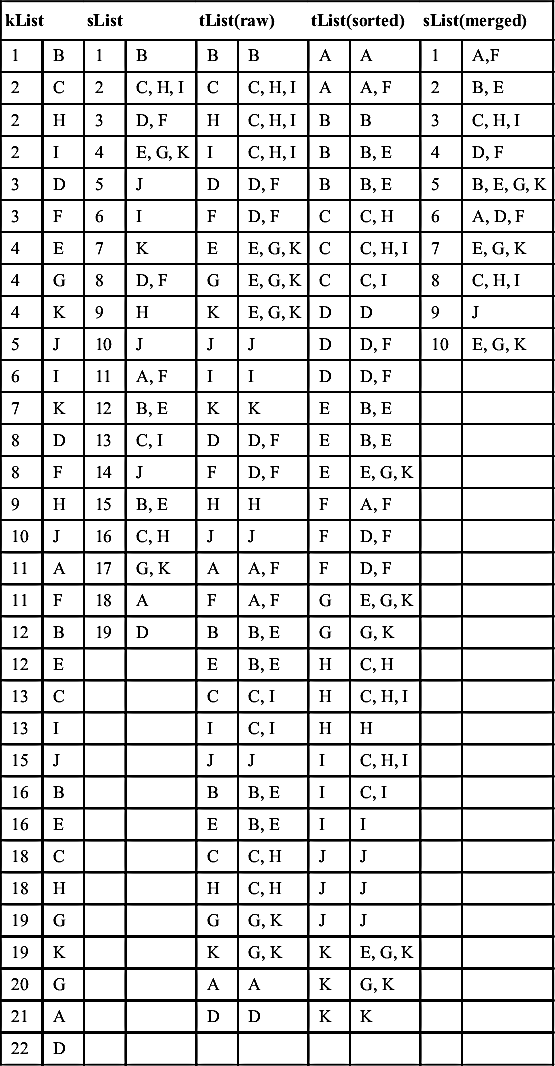
The bootstrap phase and first iteration in applying this algorithm to the match key graph of Figure 10.2 is shown in Table 10.4. The first two columns of Table 10.4 with the heading of kList show the information from Table 10.3 flattened into a single column and sorted in order by match key values. The next two columns with the heading sList show the first set of proto-components formed by collapsing the key blocks in the second column under kList. The two columns with the heading tList(raw) show the expansion step of the first iteration in which each proto-component in the input is expanded into key-value pairs.
The two columns with the heading tList(sorted) show the same key-value pairs under the heading tList(raw), but in sorted order by the key value (reference identifier). The final step of the first iteration is to merge the values (lists) in the same key-value block. This creates a list of 10 proto-components under the heading of sList(merged), which will become the input into the second iteration.
It is also important to note that in the final merge step, every key-value block changed except for the key-value block with the key value of J shown highlighted in Table 10.4.
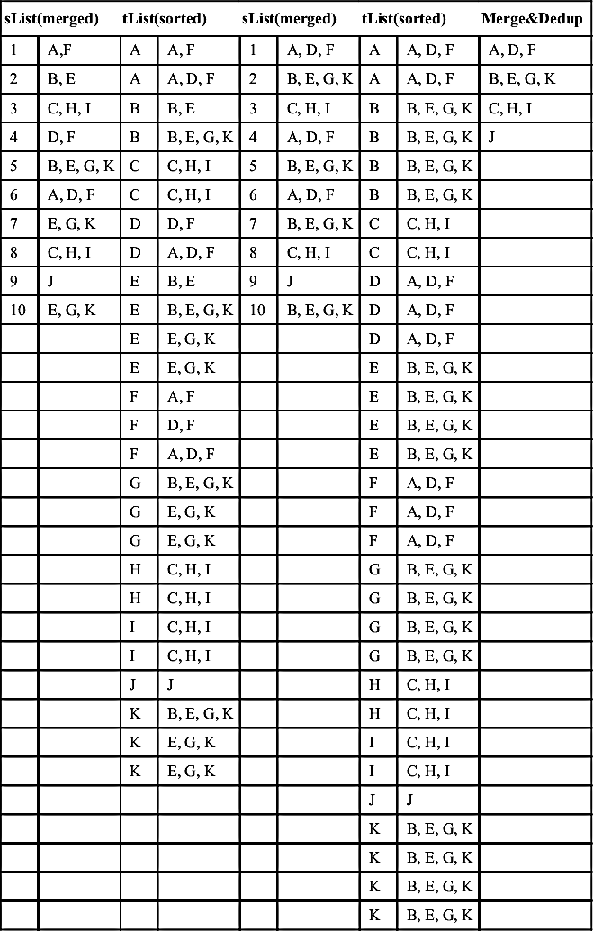
Table 10.5 shows the remaining iterations and final deduplication phase for this example. For brevity the expansion steps (tList(raw)) have been omitted as has the last merge step. The final tList(sorted) columns signal the final iteration because there are no changes in when proto-components in the same key-value block are merged. The final result comprises the four components of the match key graph shown in the Figure 10.4.
For simplicity, the pseudo-code and example shown here use the simplest form of the algorithm. In following the steps it is easy to see the many opportunities to reduce the effort. For example, whenever a proto-component has not changed during the merger, it does not need to be expanded into the next step. Its cross-product key-value pairs no longer have any contribution to make to the transitive closure of other components. Another improvement is to deduplicate the input sList before expanding the sList into the tList key-value pairs.
Iterations 2 through 3 and the Deduplication Phase
sList(merged)
tList(sorted)
sList(merged)
tList(sorted)
Merge&Dedup
1
A,F
A
A, F
1
A, D, F
A
A, D, F
A, D, F
2
B, E
A
A, D, F
2
B, E, G, K
A
A, D, F
B, E, G, K
3
C, H, I
B
B, E
3
C, H, I
B
B, E, G, K
C, H, I
4
D, F
B
B, E, G, K
4
A, D, F
B
B, E, G, K
J
5
B, E, G, K
C
C, H, I
5
B, E, G, K
B
B, E, G, K
6
A, D, F
C
C, H, I
6
A, D, F
B
B, E, G, K
7
E, G, K
D
D, F
7
B, E, G, K
C
C, H, I
8
C, H, I
D
A, D, F
8
C, H, I
C
C, H, I
9
J
E
B, E
9
J
D
A, D, F
10
E, G, K
E
B, E, G, K
10
B, E, G, K
D
A, D, F
E
E, G, K
D
A, D, F
E
E, G, K
E
B, E, G, K
F
A, F
E
B, E, G, K
F
D, F
E
B, E, G, K
F
A, D, F
E
B, E, G, K
G
B, E, G, K
F
A, D, F
G
E, G, K
F
A, D, F
G
E, G, K
F
A, D, F
H
C, H, I
G
B, E, G, K
H
C, H, I
G
B, E, G, K
I
C, H, I
G
B, E, G, K
I
C, H, I
G
B, E, G, K
J
J
H
C, H, I
K
B, E, G, K
H
C, H, I
K
E, G, K
I
C, H, I
K
E, G, K
I
C, H, I
J
J
K
B, E, G, K
K
B, E, G, K
K
B, E, G, K
K
B, E, G, K
One final observation is that the algorithm is symmetric with respect to reference identifiers and match keys. It is a simple matter to reverse the map output from the key generation so the key-value pairs input to the bootstrap have the reference identifier as the key and the match key as the value. In this case, instead of discarding the match key, the reference identifier is discarded and the iteration proceeds by performing the transitive closure on the match keys instead of the reference identifiers. If there are relatively few match key generators, then closure on the match keys can be more efficient than closure on the reference identifiers because the cross-products are smaller. The only difference is that at the end, it will take two joins to recover the original reference value, one to join the match key to the reference identifier and another to join the reference identifier to the reference value.
Although not shown in the example given in Figure 10.4, another practical problem that must be addressed is the possibility that some references will not generate a match key by any of the generators. Although this is clearly an indication of a poor quality record, it could happen for certain sets of references and match key generator configurations. One approach is to write these references out as exceptions and not carry them through the transitive closure process.
By the fact that a reference does not generate a match key value, it is already known it will not match with any other references. Therefore, references that do not generate a match key will form their own, single-reference clusters in the final output. If these references are carried forward to participate in the transitive closure process rather than output as exceptions, then they should each be assigned an autogenerated match key value. However, if they are all given the same default match, instead of forming many, single-reference clusters, they will form one large component that can degrade the overall performance of the system. In order to prevent this, the autogenerated match key should be unique across all references. In a distributed processing environment such as Hadoop, assigning a value unique across all processors in the system can be a challenge. Autogenerated keys for this purpose should use some local processor variable such as node name together with a sequence number to prevent different processors from assigning the same key value.
Example of Hadoop Implementation
The following code for the bootstrap phase of the transitive closure is implemented as a Reducer class in Hadoop. The Bootstrap reducer essentially reads the kList and creates the tList(raw) shown in Table 10.4. Note the sList in Table 10.4 is only shown for clarity. The building of the sList is not a required step in the algorithm.
The input coming into the Bootstrap reducer is a series of key-value blocks similar to the kList. Each block comprises one key and series of values. The values are presented to the reducer as an iterable list. The Bootstrap class overrides the “reduce()” method of the parent Reducer class. The first argument of the “reduce()” method is the key of the block labeled as “inputKey”. The second argument is the iterable list of values labeled “values”. The first two arguments are inputs. The third argument is the output Context labeled “context”.
/∗∗ @author Cheng @date 08/25/2014 ∗/
public class Bootstrap extends Reducer<Text, Text, Text, Text> {
The Bootstrap input is coming from a mapper that generated a set of match keys for each reference. The mapper writes its key-value pairs to its Context with the generated match key as the key of the key-value pair, and the reference identifier as the value of the key-value pair. A shuffle step prior to the reducer brings together the pairs having the same match key and block passed to the Bootstrap reducer. So for the Bootstrap reducer, the key of each key-block is a match key, and the values are the reference identifiers that produced the match key similar to the kList in Table 10.4. For example, in Table 10.4, match key value “1” was only produced by Reference B, and match key “2” was produced by References C, H, and I.
In the Bootstrap class, the first operation is to iterate over the values in the block and add each one to a Java TreeSet structure labeled “group”. A TreeSet structure is used because it will insert new items in sorted order. It is important for the operation of the algorithm that the list of reference identifiers output from each iteration step is in sorted order.
All of the values in the block are cast and manipulated as Java String objects. In the next step, the values are made into a single string that uses a Bell character as a delimiter to separate the different reference identifiers. The construction of the delimited string is carried out by the “printArray()” method. The “printArray()” method iterates over reference identifiers in the TreeSet and concatenates these values in sorted order into a string labeled “result”. All values except for the first value are preceded by an ASCI “u0007” (Bell) character. The Bell character serves as a delimiter to make it easier for the string to be parsed into individual reference identifiers at a later point in the algorithm.
After the string is constructed, the reducer writes a single key-value pair to Context where the key value is the first reference identifier in the TreeSet (“aa”) and the value is the concatenated string of all reference identifiers in the block (the “result” returned from “printArray()”). However in this code, no key-value pair is written for blocks containing only one value. Again this is departure from the example shown in Table 10.4 implemented for performance efficiency. When a match key block only contains one reference identifier, either that reference is connected to other references in another block, or the reference is not connected to any other reference. For the “1” block only containing B, it is the former. Reference B is connect to reference E in the “12” and “16” blocks of kList. Hence, reference B will be retained in the bootstrap because it is present in other match key blocks with more than one value.
However, some references may be lost entirely during bootstrap because they do not connect with any other reference. For example, the reference J only occurs in the kList in the single-value blocks “5”, “10”, and “15”. Therefore, the reference J is lost during bootstrap. However, this is not a problem because the final step of the transitive closure process is to perform an outer join between the reference identifiers remaining at the end of the transitive closure process with the original input of reference identifier-reference pairs. Because it is an outer join, all of the original references will be recovered at the end of the process. It will also signal that any reference recovered by the outer join will form a single-reference component of the graph.
ER Using the Null Rule
It is important not get lost in the details of the transitive closure process and lose sight of the overall objective, which is ER. As shown in Figure 10.2 the transitive closure is only an intermediate step to partition the set references to be resolved into manageable sized blocks. In this case the blocks are the connected components of the match key graph of references. Each component becomes the input to an ER process which applies an ER algorithm and matching rule to find the clusters and create the final set of EIS.
However, there are situations where it is possible to end the ER process with transitive closures. This is possible when the match rule is a Boolean rule set, and where each one of the comparators used in the rules are hash functions. In this case, match key generators can be constructed in such a way that they are equivalent to the match rules. In other words, two references share the same match key if, and only if, the references match by the rule that corresponds to the match key. In this case the components found from the transitive closure of the match keys represent the final clusters of the ER process, and the ER process is said to use the “Null Rule.”
Here is a simple example. Suppose an ER process for matching student records uses a two-part Boolean rule. The first part is two enrollment records are a match if they agree on first, middle, and last name values. The second part is they are considered a match if they agree on the last name, have the same date-of-birth, and the first names agree on Soundex value. Since simple agreement (exact match) and Soundex agreement are both hash function comparators, then the enrollment records can be resolved using the null rule.
To use the null rule for this example requires building two match key generators, one for the first rule that creates a match key by concatenating the characters of the first, middle, and last names (presumably with some cleansing such as upper casing and removing punctuation). The second match key generator would create a match key by concatenating the four-character Soundex value of the first name with the character of the last name and digits of the date-of-birth (again with some cleansing and standardization). So, clearly if two enrollment records share one of these keys, the records are going to match according to the rule that corresponds to the key. Therefore, a component formed by the transitive closure of the enrollment records by these two match keys contains all of the records that are equivalent by the Boolean match rule.
The null rule cannot be used if any of the comparators of the proposed matching rule are similarity functions rather than hash functions – for example, comparators such as Levenshtein edit distance or Q-gram. In these cases, the match keys can only approximate the match conditions up to hash function levels. The final components from the transitive closure of the approximate match keys must be further refined by applying the full match rule.
Using the previous example, suppose the second part of the rule were changed to require the first name values to be within one Levenshtein edit distance of each other instead of having the same Soundex value. Now the second match key generator would have to be revised. Because Levenshtein is a similarity function rather than a hash function, the new index generator would have to omit the first name and only concatenate the last name and date-of-birth. However, this change would now allow enrollment records with completely different first names to come into the same component as long as they agree on last name and date-of-birth. Therefore, the references in these components would have to be compared using the complete match rule in order to make the final determination of clusters.
The Capture Phase and IKB
The only thing that differentiates merge-purge ER from the capture phase of CSRUD is the transformation of clusters into EIS and storing them in an IKB. The flows in Figures 10.1 and 10.2 are essentially the same for both except for capture, the merged output from the ER flow into a storage system. In the distributed processing storage environment, both the Hadoop File System (HDFS) and HBase follow the key-value pair paradigm. Because they do not follow the relational data base model and do not directly support structure query language (SQL) they are often referred to as “Not only SQL” or NoSQL databases. Following the Hadoop model for distributed process used up to this point, the design for a distributed IKB will follow an HDFS file system implementation.
In order to retain the full functionality present in a nondistributed file system, a distributed IKB requires a number of tables, except that in HDFS tables correspond to folders. Again each folder contains one set of key-value pairs and possibly other folders. Because it is a distributed file system, HDFS only presents the user with a logical view of a file as a folder. Underneath the folder HDFS may be managing the physical file as segments distributed over several different underlying storage units. Figure 1.3 in Chapter 1 shows a segment of a nondistributed IKB created in a capture configuration of the OYSTER ER system. OYSTER stores its IKB as an XML document with a hierarchical structure. The IKB comprises the IKB-level metadata (<Metadata>) and the EIS (<Identities>). Each EIS (<Identity>) comprises a set of references (<References>) that in turn comprise a reference value (<Value>) in CoDoSA format and reference metadata (<Traces>).
In the HDFS distributed data store, both data and metadata reside in folders created by map/reduce processes. Each folder corresponds to a logic dataset comprising key-value pairs. The physical segments of the dataset may actually reside in different locations managed by HDFS.
There are three essential key-value folders in the HDFS version of the IKB. The text in parentheses after the name of the folder describes the key-value pair definitions for the folder.
• References – (Source identifier + Reference identifier, reference value) the store of all references under management. Note the key value is a concatenation of the source identifier for the reference with the unique reference identifier within the source. This is required to give each reference in the IKB a unique identifier across all sources. The reference value is a CoDoSA encoded string where each attribute value is preceded with an escape character (ASCI Bell) followed by an attribute tag. The meaning of the attribute tag is defined in the CoDoSA Tags table of the IKB.
• Entities – (Entity identifier, Entity-level metadata) The key is the entity identifier and the value is a string that is a concatenation of various entity-level metadata items such as the identifier of the run (process) in which the entity was created and the identifiers of any runs in which the entity was modified. This is where any assertion metadata would be stored as well as including true positive assertion tags and negative structure-to-structure assertion tags generated by correction or confirmation assertions as discussed in Chapter 5.
• Reference-to-Entity – (Source identifier + Reference identifier, Entity identifier + Reference-level metadata) Key-value pairs in the Entities folder have the same key as the References folder, but have a different value structure. The value string is a concatenation of the entity identifier and various reference-level metadata. The primary purpose of the Entities folder is to indicate for each reference the entity to which it belongs. This folder defines the EIS of the IKB. All of the references with the same entity identifier comprise an EIS. The remaining portion of the value string following the entity identifier contains various metadata pertaining to the relationship between the reference and the entity to which it belongs. For example, the reference-level metadata could include the identifier of the run (process) in which the reference was merged into the EIS. It might also include the identifier of the rule that caused the reference to merge into the EIS.
There are several additional folders that can be added to the IKB. These folders are primarily to hold IKB-level metadata and are generally small enough that they can hold physical tables (text files) rather than virtual key-value pairs. These include
• Run Identifiers – A sequence number or other unique identifier for each run of the system for traceability and auditing. Run identifiers are primarily used to associate other metadata with a particular run of the system.
• CoDoSA Tags – A two-column table where each row has a CoDoSA attribute tag followed by its description. These tags are used to encode the string representing the reference value in the References folder.
• Sources – A four-column table where each row has a unique source identifier, path to the source, name of source, and description of the source.
• Other tables to store copies of the Run Scripts (control scripts) for each run, Reports generated from each run, log files generated for each run, and any other run-level metadata.
The Identity Update Problem
Another important EIIM configuration is the automated update configuration in the update phase of the CSRUD Life Cycle. When new references are introduced, the system uses the matching rule to decide if each new reference is referring to an entity already represented in the IKB by an existing EIS, or if it is referring to some new entity not yet represented in the system. In the former case, the system should integrate the new reference into the EIS of the matching identity. In the latter case, the system must create a new EIS and add it to the IKB to represent the new identity. This means there will be two inputs to the update process including the existing (prior) EIS created in a previous process and the new references.
Figure 10.5 The basic workflow for the update configuration.
Figure 10.5 shows the general approach to the update configuration for a distributed processing environment that is basically the identity capture workflow of Figure 10.4 with an added input of prior EIS to be updated.
One problem in adapting the identity capture workflow of Figure 10.4 to identity update is that the identity capture workflow was based on the assumption that all of the inputs are single references, each with a unique reference identifier, but in Figure 10.5 the Prior input comprises EIS rather than references.
If the Prior EIS have a record-based structure, then it is possible to recover (reconstruct) the references used to create each of the prior EIS. If not, then it may still be possible to recover these references as long as the aggregate set of references used to create the Prior EIS has been saved or archived in some way. In either case it means the workflow in Figure 10.5 is essentially a recapture of the prior references combined with the new references.
However, there are still two problems with the recapture approach. The first issue concerns the evolution of matching rules. Over time, the matching rules may be modified to improve the entity identity integrity of EIS or to accommodate changes in the reference data. Therefore, the matching rules used to create or update the prior EIS may be different from the matching rules currently in effect. A simple recapture process will apply the current identity rules to the prior references as well as the new references. In other words, the identities represented by the prior EIS from D are essentially discarded, and the identities represented by the EIS in E are based entirely on the current rules. This issue may or may not be a problem, but it is an artifact of the recapture approach that should be noted.
The second problem in using a recapture approach is a much more fundamental issue related to the issue of persistent identifiers for the identities represented in the system.
Persistent Entity Identifiers
An important goal of EIIM is to create and maintain persistent entity identifiers for each identity under management, i.e. each EIS retains the same identifier from process to process. This is not the case for basic ER systems that do not create and maintain EIS. In these systems the link identifier assigned to a cluster of references at the end of the process is transient because it is not part of a persistent identity structure. The entity identifiers assigned by these systems are only intended to represent the linking (identity) decisions for a particular process acting on a particular input. Typically these system select one survivor record from each link cluster to go forward into further processing steps. After the survivor record has been selected, the link identifier is no longer needed.
If the only objective were to build the identities represented by combining the references from Prior EIS with the new references, then a recapture approach to the workflow shown in Figure 10.5 would be sufficient. The problem is even though the EIS in the merged output bring together all of the references that represent the same identity, a Prior EIS and a corresponding EIS in the output that represent the same entity may be assigned different identifiers. In other words, from an EIIM perspective, simply performing a capture process on the combined references would have the undesirable side effect that the identifiers for the same entity identity could change after each update process.
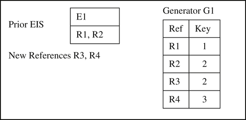
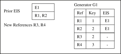
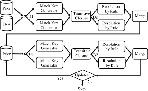
Fortunately, there is a fairly simple solution to the problem, and that is to treat the EIS identifier as a match key in the transitive closure process. To see how this works, consider a simple example in which there is only one Prior EIS, one new reference, and a single match key generator G1 as shown in Figure 10.6.
In the scenario of Figure 10.6 there is a single Prior EIS with Identifier E1 that comprises two references R1 and R2, two new reference R3 and R4, and a single match key generator G1 that produces three distinct match key values 1, 2, and 3. For purposes of the example, assume the generator G1 is aligned with the base match rule, and R2 and R3 match by the base rule. Remember the alignment between the match rule and the generator means if two references match they must generate the same match key; however, if they generate the same match key, they do not necessarily match by the rule.
Also, notice in the scenario of Figure 10.6 that R1 and R2 do not generate the same match key even though they are in the same EIS. Assuming generator alignment, this means R1 and R2 do not match by the base rule because they generate different match keys. However, it is important to remember EIS are designed to store equivalent references and not all equivalent references match. For example, suppose these are customer references and the base rule is they must match on name and address. The references R1 and R2 may be for the same customer who has changed address, i.e. the address in R1 does not match the address in R2. If the generator G1 is aligned with the name+address match rule, then it is unlikely the hash value produced by the address in R1 will be the same as the hash value produced by the address in R2; consequently the match keys for R1 and R2 will be different.
Figure 10.6 Simple update scenario.
Nevertheless, these references are equivalent and therefore belong in the same EIS. This EIS may have been formed in a previous automated ER process that used a different base rule, e.g. match on name and telephone number, or these references may have been asserted together in a manual update process.
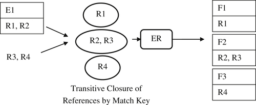
Given these assumptions, then a simple capture process on the combined reference would result in three output EIS shown in Figure 10.7 as F1, F2, and F3.
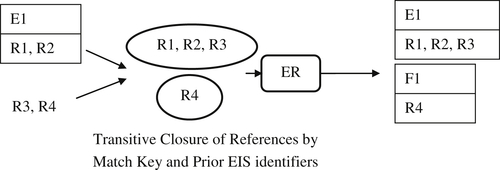
The problem is the result shown in Figure 10.7 is incorrect. Given R1 and R2 are equivalent, and R2 matches R3, then by transitive closure of equivalence, R1, R2, and R3 should all be in the same EIS. In order to solve the problem, the knowledge of prior equivalence must be carried forward into the preresolution transitive closure process. This can be accomplished by treating the Prior EIS identifiers as supplemental match keys, as shown in Figure 10.8.
If the transitive closure of the references is determined based on both the match key and the EIS identifier, then the graph will only have two components {R1, R2, R3} and {R4}. This is because R1 and R2 are connected by the shared identifier E1, and R2 and R3 are connected by the shared match key 2. Thus, R1, R2, and R3 form a single connected component.
In order to complete transformation of the capture process into a proper update process, two more changes must be made. The first is that not only should the Prior EIS identifiers be used to form the transitive closure of the references, but also these identifiers need to be carried forward into the ER process. In other words, when the ER process sees a reference, it also needs to know if it came from a Prior EIS, and if it does, it needs the Prior EIS identifier value.
Figure 10.7 Results of capture based on transitive closure of match keys.
Figure 10.8 Simple update scenario with supplemental EIS keys.
Secondly, the matching logic of the ER process needs to be augmented. Regardless of the base match rule, any time two references are determined to have come from the same Prior EIS, they should be considered a match. In other words, the base match rule is supplemented with an assertion rule. Furthermore, the EIS created by the ER process should reuse the Prior EIS identifiers in those cases where the output EIS contains a reference from a Prior EIS.
Figure 10.9 shows the correct result obtained by making these three changes, i.e. adding the Prior EIS identifier as a supplemental match key for transitive closure, carrying the Prior EIS identifier forward into the ER process, and augmenting the ER base rule with the assertion rule for references originating from the same Prior EIS. Note the first output EIS has been labeled with the Prior EIS identifier E1 because it represents the same identity updated with a new reference R3. On the other hand, F1 represents a new identity formed by the reference R4.
In the example shown in Figure 10.8, one component has a reference from a Prior EIS together with a new reference, and the other component has only a new reference. In general there can be four situations that occur:
1. If the component contains only references from one Prior EIS, it means there are no new references that share a match key value with the references in the prior EIS. The result is that the prior EIS will not be modified by the update process. It will pass through unchanged and retain its original identifier.
Figure 10.9 Correct update of the simple scenario of Figure 10.6.
2. If the component contains references from one prior EIS along with new references, then there is the potential that the Prior EIS will be updated. However, this is only a potential update because sharing a match key only means a match is possible, not guaranteed. Whether a match actually occurs will not be known until the component goes into the ER process where pairs of references are tested by the match rule. If none of the new references in the component match one of the references from the Prior EIS, then the new references will form one or more new EIS in the output.
3. If the component contains only new input references, then the references will not update any Prior EIS. Instead they will form one or more new EIS in the output that will be assigned new identifiers.
4. It is possible a component could include references from more than one Prior EIS. This would happen if one of the new references shares a match key with references in two or more Prior EIS. If the new reference that shares a match key turns out to actually match the references in the Prior EIS, then by transitive closure of equivalence, the EIS should be merged into a single EIS. The exception to this is when the EIS have been previously split by an assertion. EIS formed by a split assertion process are cross-referenced to prevent them from merging during an automated update process.
The Large Component and Big Entity Problems
Although identity capture and identity update workflows, described in Figures 10.2 and 10.5 respectively, can be operationalized using preresolution transitive closure, they will only work well when the match keys are similar to, or the same as, the matching rule. The problem is not with logic of the system, but in interaction between the software and the data, the root of many data process problems (Zhou, Talburt, & Nelson, 2011). In the case of the preresolution transitive closure algorithm, the problem is the components (blocks) can become very large and overwhelm the capacity of the system even in a large-scale, distributed processing environment.
An example of how components can grow very large was described in Chapter 9 in the section “Dynamic Blocking versus Preresolution Blocking.” In the CDI example only two match keys were defined – a first name match key and a last name match key. The transitive closure of these two match keys will likely grow into one component that includes every reference, a result that defeats the purpose of blocking. As described in Chapter 8, in the section “Cluster-to-Cluster Classification,” reference equivalence is transitive, but reference matching is not transitive. The clusters formed by the ER process are the transitive closure of the reference-to-reference links made by the matching rules under the assumption that matching references are equivalent references.
However, two references that agree on a match key value are only potential matches and, consequently, are only potentially equivalent. As chains of references connected by common match key values continue to grow in the transitive closure process, the references at the extreme ends of the chain are less likely to match. Again using the first and last name match key example, “James Doe” and “Mary Doe” connect by last name, “Mary Doe” and “Mary Smith” connect by first name. However, “James Doe” and “Mary Doe” at the ends of the chain are not good match candidates even though they will be placed into the same component by the transitive closure of the two match keys. Given a set of match key generators, it is hard to predict how they will interact without actually starting the transitive closure process and observing the growth of the components.
To solve the problem of large components, the transitive closure process and the matching process must somehow be blended together to constrain the growth of the chains that create the large components. There are many different strategies for controlling this growth (Kardes, Konidena, Agarwal, Huff, & Sun, 2013; Kolb, Thor, & Rahm, 2011; Papadakis, Ioannou, Niederée, Palpanas, & Nedjl, 2012). Two described here are postresolution transitive closure and incremental transitive closure.
Postresolution Transitive Closure
The strategy of postresolution transitive closure is to translate each match key into an entity identifier and then perform the transitive closure on the entity identifiers. The process is illustrated in Figure 10.10.
In this process the same set of references (Ref) is resolved multiple times, one time for each match key (M-Kx). Each of these single match-key flows corresponds to Figure 10.1 where blocking takes place using only one match key. However, the ER process uses a full set of matching rules (or at least all of the matching rules that align with the match key), so the clusters formed at the end of each resolution step comprise only equivalent references. In the transitive closure process, the chaining takes place on the entity identifiers assigned to each reference rather than on the match key. Because a shared identifier represents equivalence instead of a possible match, the components formed in the closure process are actually the EIS that would be formed using all of the match keys and matching rules in one ER step. Therefore, the components in the postresolution transitive closure are constrained to be no larger than the largest entity that can be formed by the matching rules.
Figure 10.10 Postresolution transitive closure.
The advantage of postresolution transitive closure is the maximum size block for each match key is known in advance, and the growth of the components in the final transitive closure is constrained to only chain equivalent references. The disadvantage of this approach is if N is the number of match keys, then the full set of input references must run N times, and the input to the final transitive closure is N times the size of the original set of input references.
Incremental Transitive Closure
Another strategy is similar to the update process shown in Figure 10.4. Here the idea is to blend each match key into the transitive closure process with the equivalences found by previously processed match keys. The process is illustrated in Figure 10.11.
The incremental transitive closure process starts in the same way as postresolution transitive closure where the ER process uses only the first match key generator. In the second step, the entity identifier assigned to each reference by the ER process is appended as an additional attribute to each of the original references. In addition, the next match key generator is applied, so each reference has two match keys – the entity identifier from the previous ER process and the match key from the next match key generator. The transitive closure operates on these two keys followed by the full ER process that assigns a new set of entity identifiers. This process continues until all of the match keys have been processed.
Figure 10.11 Incremental transitive closure.
The advantage of the incremental process is both the transitive closure process and the ER process can be highly optimized. In the transitive closure process, the bootstrap phase can take advantage of the previous matching. For example, if a group of references sharing the next match key also has the same identifier from the previous ER process, then the group does not need to go through the closure process because the match key is not adding any incremental value. It is not bringing together any references that have not already been determined as equivalent. Similarly in the ER process, any references already determined to be equivalent in a previous ER process (i.e. share the same entity identifier) do not need to be matched again. Matching only needs to take place between references that have different entity identifiers while sharing the same match key.
The Big Entity Problem
Aside from the problem of large components (blocks), there can also be a problem when some entities cluster a large number of references, so-called big entities. Sometimes a big entity is just a big entity because it really does comprise many references, but sometimes it is caused by data quality issues.
In the former this is sometimes caused by a client system repeatedly sending an entire set of references to the hub rather than only new references. For example, in student tracking the enrollment system may send the records of all students enrolled every day. Although a few of these may be new or changes, the vast majority are the same from day to day. This can be a problem for MDM systems that store every reference. For these cases the system implements logic for recognizing and handling duplicate records of previous inputs such as the duplicate record filter shown in Figure 4.4 in the section “Dedicated MDM Systems” in Chapter 4.
The data quality issues that cause big entities are often related to default values. Instead of leaving fields blank, many data entry systems are written to either automatically provide a default value or default values are entered by the operator because an entry is required by the software. For example, the entry of “LNU” for last name unknown or “999-99-9999” for a missing social security number. The problem is that when these fields are used as identity attributes in the ER process they can sometimes cause big entities to be formed. Again, the answer is usually a special filter that recognizes and handles default values in the matching process.
Identity Capture and Update for Attribute-Based Resolution
Everything described to this point has assumed the ER systems are using record-based architecture, i.e. record-based projection and record-based EIS as described in Chapter 8. In the case of attribute-based resolution, the purely sequential workflows given so far will not always work correctly. The reason is that, when an EIS is updated to include a new reference, the introduction of the new information may cause the updated EIS to match other references that it did not match prior to the update. This creates a problem for the preresolution transitive closure method. For example, in workflows such as those shown in Figures 10.2 and 10.5, the transitive closure operations are based on shared match keys and, for update, on shared EIS identifiers. However, the match keys used in the closure are generated from the new references and Prior EIS before starting the ER process. In a record-based ER architecture this is not a problem. As long as the match key generators are in alignment with the base matching rule, each connected component will contain all of the new references and Prior EIS that potentially match.
However, in the case of an attribute-based architecture, if a reference updates (i.e. is merged into) an EIS during the resolution process, the updated EIS can potentially generate new match key values that would not have existed before the update. These new, postresolution match key values may connect the updated EIS with other input references or other EIS not included in the component during the transitive closure process because the closure process took place before the EIS was updated.
One solution for the attribute-based resolution problem is to simply iterate the preresolution update workflow as shown in Figure 10.12. This workflow already assumes EIS from previous processes are (or can be) included as part of the input. If any prior EIS are included in the input, then index values are generated for these EIS by the IXG processes before starting the transitive index closure step.
In the case of attribute-based resolution, the first step is the same as for record-based resolution. The set of new references and any prior EIS are the inputs that produce the updated EIS. However, if any EIS were updated during the initial phase, it is necessary to rerun the output EIS as input to a second, iterative step.
Figure 10.12 Iterative update process for attribute-based ER systems.
In the iterative step, all of the match key values are generated for the EIS followed by the transitive closure process and the resolution process. If during the resolution process some of the EIS are updated, the EIS must be processed again. This is repeated until there are no updates. The same process as shown in Figure 10.12 also works for attribute-based identity capture. The only difference is the input to the first step is only the set of new references, and there is no set of prior EIS.
Concluding Remarks
MDM for Big Data is difficult but possible using distributed computing. The two biggest problems to solve for distributed MDM are transitive closure and update. If an ER process only requires a single blocking key, then the distributed processing flow is quite simple. The key blocks of a single key partition the references, and the partition segments form natural key-value blocks that can be allocated to distributed processors. However, if more than one blocking key is used, there must be a transitive closure process. The transitive closure can occur at different points in the ER process – prior to matching (preresolution), after matching (postresolution) or intertwined with the matching process (incremental). The choice of strategy will be dictated by the nature of the data. The transitive closure process finds the components of the graph formed from reference nodes connected by edges of shared match key values. One advantage of pretransitive closure is the components of the match key graph represent the final set of clusters when the ER match rules are the same as the match key generation rules (null rules). Otherwise, the match key components must undergo a final resolution at each node using the full and complete set of matching rules. The greatest disadvantage to preresolution transitive closure is that for certain match key combinations it can create very large components too large to process. When this happens, a different strategy for transitive closure must be used.
In order to implement the full CSRUD MDM Life Cycle, the basic process capture process must be modified to allow for update. Update requires that both new references and old (previously clustered) references be input into the preresolution transitive closure process. Moreover, to preserve previous clustering decisions and maintain persistent entity identifiers, the old references must also carry along their previously assigned entity identifiers. This serves two purposes. The first is to retain and reuse the previous identifier whenever possible. The second is to preserve linking decisions from previous update processes. The previously assigned identifiers are input into the transitive closure process and treated by the transitive closure process the same as if they were generated match keys. In the case where the ER process is using an attribute-based project for cluster matching, the entire transitive closure/ER process must be repeated until no new clusters are formed.