
Appendix A
Some Commonly Used ER Comparators
Exact Match and Standardization
The most fundamental and most commonly used similarity is an exact match between two values. Exact match requires both values to be the same according to their data type, i.e. the same numeric value, the same date, or the same string.
In the case of string values, exact match is a demanding requirement. Two strings will only be exactly the same if they comprise exactly the same characters (by internal character code) in exactly the same order. For example, while “JOHN” and “JOHN” are exact string matches, the strings “JOHN” and “John” are not. The character code for an upper case “O” is different from the character code for a lower case “o”. The same is true for the letters “H” and “N” as well.
Similarly, the strings “JOHN R. DOE” and “JOHN R DOE” are not an exact match because the first string contains a period (“.”) and the second does not. However, in both cases most people would consider these a match in the sense that they essentially represent the same name value. For this reason, when string values are compared they generally are subject to some alteration or standardization so that two strings representing the same underlying value will also be the same string value. The two examples given here are two of the most common standardizations used for string values, i.e. standardizing letter case and removing punctuation.
Where to Standardize
There are two schools of thought on standardization of values. The first and most common is that standardization should be done in a separate process prior to the ER matching process. The other is that the comparison operators themselves should compensate for the differences. There are pros and cons to each approach. Preprocess standardization has the advantage that each value is transformed one time rather than having to be transformed each time it is used in a match operation. Preprocess standardization also often makes it easier to apply more complex transformations than having to build these into the code of the comparator logic.
However, there are two disadvantages to preprocess standardization. The first is that it creates a dependency between preprocess and the ensuing ER process. For the same set of input references, the ER process may deliver different results when there are changes to the standardization. This makes it difficult to understand the true action of the matching rules without first understanding preprocess standardization. Often this information is in two different places and may even be administered by different groups. If the standardization is built into the matching rules, then it is easier to manage the dependency between standardization and matching.
A second reason why it may be better to standardize in the comparator is a fundamental rule of data management – always keep the original data. For example, if the EIS is built from standardized data, then it is more difficult to know the true states of the original references from which the EIS was constructed.
Overcoming Variation in String Values
So regardless of where standardization takes place, in preprocess or in the comparator logic, the goal is to overcome variations between two representations of the same underlying value. This is primarily a problem with values represented as string or character data types. Seven of the most common types of variation are:
1. Format variation – the characters that represent the value are the same, but they are couched in different formats. For example, two telephone numbers with exactly the same 10-digit sequence, but represented as “(012) 345-6789” versus “012.345.6789”. This also includes standardizing letter casing and spacing.
2. Damaged value – even after removing format variation, the values are slightly different strings due to some type of input or process error that has removed, changed, inserted, or transposed characters. For example, “Johnson” versus “Jhonson”, a common typing error.
3. Alias value – these are strings that can be entirely different, but semantically they mean the same thing. This is common with names such as “Robert” and “Bob” but also common in addresses with the use of abbreviations such as “Av” for “Avenue” or “MLK” for “Martin Luther King”.
4. Phonetic variation – these are strings that when pronounced as words have a similar sound. Phonetic variations often occur when data are transcribed from speech such as on orders taken by telephone. For example, “Christy” versus “Kristi”.
5. Alternate value – these are cases where there can be more than one valid value to represent an attribute. They often occur as the result of a name or address change or different usages in different contexts. For example, “Jane Doe” becomes “Jane Smith” after marriage.
6. Misfielding – this variation occurs when valid values are misclassified by attribute name. Common examples are name reversals where the first name value has been recorded in the last name field, and the last name value in the first name field. Similar misfielding often occurs with home telephone number versus work telephone number.
7. Missing value – there is no meaningful value present. They may be missing because the value is null, empty, or blank. However, a missing value can also occur when a placeholder value is used to overcome data entry restrictions. For example, if telephone number is a required entry, but was not known when the data were recorded, the person entering the information may simply enter a value like “999-999-9999” in order to proceed to the next screen. Even though missing values cannot be easily overcome, it is important to know which attributes have missing values and to what degree the values are missing. Placeholder values can be harder to detect and can do more to lower matching accuracy than blank values. The reason is because they can cause a match between identity attributes when in fact they should not match and lead to false positive links.
Scanning Comparators
Scanning comparators are used to address format variations. Scanning comparators examine a string character-by-character looking for particular characters that should be changed or removed. For example, a comparator like ExactIgnoreCase will search for and replace each lower-case letter in a string with its corresponding upper-case character before comparing the two strings. By using the ExactIgnoreCase comparator the example strings “JOHN” and “John” will match.
Sometimes more sophisticated scanning comparators are used that can perform several types of operations in the same scan of the string. For example, the CharScan(A, B, C) comparator that takes three arguments where
A Indicates the type of characters to retain, but omitting all other characters, e.g. letters, digits, letters & digits, etc.
B Indicates the maximum number of characters to keep
C Indicates when retaining letters whether lower-case letters should be converted to the corresponding upper-case character, or to keep them in their original case
For example, CharScan(Letters, All, ToUpper) would overcome the variation between the strings “John R. Doe” and “JOHN R DOE” by ignoring the blanks and the period while also changing the lower-case letters to upper-case. The final comparison would be between “JOHNRDOE” and “JOHNRDOE”, resulting in an exact match.
It is important to note the transformations performed by the comparator do not change the original values of the string. They only create proxy strings, sometimes called hash values, for comparison purposes. The hashed values are discarded after the final comparison is made.
Approximate String Match Comparators
To get beyond format variation and overcome damaged values, more sophisticated comparators are required. There is a large family of approximate string matching (ASM) comparators that judge the similarity between two strings in terms of the number or order of shared characters.
Transpose
One of the simplest ASM comparators is Transpose. The Transpose comparator returns a match signal whenever two strings differ by the transposition (reversal) of two adjacent characters. The transposition of two characters is a common keyboard entry error. For example, the strings “Jhon” and “John” will be considered a match by the Transpose comparator.
One could argue that if two strings are identical, the Transpose should also consider them a match as well. However, this is generally not the case. Most comparators that look for special conditions such as transposition generally do not match strings where the condition is not present. This is particularly true for systems using Boolean rules. The reason is that it allows the rule designer to isolate particular match conditions to specific rules.
Take, as an example, a situation where an exact match on the values of two attributes A and B is sufficient to link the references. However, it may be observed some false negatives are created by this rule because some values of A that should match vary by transposition. In order to convert these cases to true positives a second rule is added that requires a transposition match on the A attribute values match while still requiring an exact match on the values of B. However, because the transposition is a “softer” match it could possibly cause a false positive if, by chance, two different values of A that should not match differ by a transposition not the result of a typing error. To compensate, the second rule may be augmented by requiring some level of match on a third attribute C. The two rules allow the rule designer to separate these two issues, one where both A and B are an exact match, and the other where B is exact and A is a transposition match.
Initial Match
Another useful ASM for name matching is the Initial match. Like the transposition it only creates a match in specific circumstances. Generally the condition for an Initial match is there are two strings where one string comprises a single character and the other string comprises two or more characters. If the single character in the first string is the same as the first character of the second string, then the two strings are considered an Initial match.
Again, like transposition it does not signal match in other situations, such as when two names start with the same character or when both strings are a single character. For example, the strings “J” and “John” would match by Initial, but “Jon” and “John” would not.
Levenshtein Edit Comparator
Perhaps one of the most famous and used ASM comparators is based on the Levenshtein edit distance (Levenshtein, 1966). The Levenshtein edit distance between two strings is the minimum number of basic character operations required to transform one string into the other. Typically, the allowable operations are inserting a character, deleting a character, and replacing (substituting) a character, although some versions also allow transposing two adjacent characters. For example, the string “ALISA” and “ALYSSA” are separated by an edit distance of 2 because it requires at least two transformations to transform one string into the other. For example, starting with “ALISA”, one transformation is replacing “I” with “Y” giving “ALYSA”. The second transformation is to insert an “S” giving “ALYSSA”.
By its definition the Levenshtein edit distance between two strings cannot exceed the length of the longest string. If L(A, B) represents the Levenshtein edit distance between two strings A and B, then the normalized edit distance NL can be calculated as (Christen, 2006):
![]()
Maximum q-Gram
Another family of ASM algorithms focuses on the ordering of the characters. These are called q-Gram or n-Gram algorithms. A q-Gram is a fixed sequence of characters of length q. For example, “ARM” is a 3-gram. The simplest q-Gram comparator is the Maximum q-Gram comparator. It is simply the length of the longest substring (q-Gram) shared by both strings. It is also normalized by dividing by the length of the longest string.
For example, the Maximum q-Gram similarity between “CRANSTON” and “RANSOM” is 0.5. The longest shared substring is “RANS” with length 4. The longer string “CRANSTON” has length 8, hence the Maximum q-Gram similarity is 4/8 or 0.50.
q-Gram Tetrahedral Ratio
The principle of q-Gram similarity between two strings can be extended in several ways. One way is to count the number of characters in all shared q-Grams. The more q-Grams they share, the more similar the strings. Consider the two strings “JULIE” and “JULES”. These two strings share four 1-Grams, the single letters “J”, “U”, “L”, and “E”. They also share two 2-Grams of “JU” and “UL” and one 3-Gram of “JUL”. Whereas the Maximum q-Gram only counts the longest, in this case 3, the q-Gram Tetrahedral Ratio (qTR) algorithm (Holland & Talburt, 2010b) scores the number of character as shared q-Grams against the total number possible. The total number of characters contained in all q-Grams (substrings) of a string of length N is the tetrahedral number of N given by:
![]()
In the example above, the string “JULIE” of length 5 has 15 possible substrings containing a total of 35 characters, i.e. TN = 35. As noted above, “JULIE” shares 7 of these q-Grams with “JULES” with a total of 10 characters, so the q-Gram Tetrahedral Ratio of “JULIE” with respect to “JULES” gives
![]()
In the case where the strings being compared are of different lengths, then the calculation of qTR will depend upon which string is selected to determine the tetrahedral number in the denominator of the ratio. To address these cases and make the qTR measure symmetric, an adjusted qTR measure is defined as the weighted average of the two directional measures (Holland & Talburt, 2010b). If N represents the length of the first string, M the length of the second, and Q the number of q-Grams shared by the two strings, then the adjusted qTR is given by
![]()
Jaro String Comparator
Another q-Gram variant is the Jaro String Comparator (Jaro, 1989). It considers the number of characters in common between two strings and the number of character transpositions. If A and B represent two strings with at least one character in common, then the Jaro similarity is given by
![]()
where W1, W2, W3 are the weights assigned to the first string, second string, and transpositions, respectively, and where W1 + W2 + W3 = 1, where C is the common character count, T is the number of transpositions, and LA and LB are the lengths of the two strings. For example, the strings “SHAKLER” and “SHAKEL” have 6 characters in common and one transposition of “LE” to “EL”. Assuming three equal weights of {1/3} each, the Jaro Similarity between these strings would be
![]()
Some implementations of the algorithm not only require sharing the same sequence of q characters, but also require that the shared sequences both start at the same or almost the same position in the strings. These types of q-Grams are called positional q-Grams.
Jaro-Winkler Comparator
The Jaro-Winkler Comparator (Winkler, 1999) is an example of a positional q-Gram algorithm. The Jaro-Winkler comparator is a modification of the Jaro Comparator that gives additional weight to the agreements on the first four characters of the two strings. If N represents the number of the first four characters that agree, then the Jaro-Winker similarity is calculated as
![]()
In the example of “SHAKLER” and “SHAKEL” the value N is 4. The Jaro-Winkler similarity of these two strings is calculated by
![]()
The Transpose, Initial, Levenshtein, Maximum Length q-Gram, Tetrahedral Ratio, Jaro, and Jaro-Winkler are only a few examples of the many ASM algorithms that are used in ER matching processes. A quick search of the Internet using the keywords “approximate string matching” will reveal many others along with details of their implementation.
Token and Multivalued Comparators
Most of the ASM comparators are based on comparing a single string value to another string value. However, there are many cases where a string represents multiple values – for example, a name field given as “John R. Doe”. Rather than representing a single value, this string contains several values: a first name value, a middle name value, and a last name value. The substrings of “John R. Doe” separated by spaces or punctuation are called tokens. In the example there are three tokens: “John”, “R” and “Doe”.
Jaccard Coefficient
The Jaccard Coefficient is perhaps the most canonical similarity measure. In its most general form, it compares the similarity of two sets P and Q with the following formula:
![]()
The Jaccard Coefficient can be applied at two levels. For multivalued fields, such as an address or complete name, P and Q can be sets of tokens. For example, the Jaccard Coefficient for values “Dr Sean Doe” and “John Sean Doe” is calculated by first tokenizing the two fields.
![]()
The Jaccard Coefficient can also be applied at the character level. For example,
![]()
The advantage of the Jaccard Coefficient for token comparison is it is not sensitive to word order because it considers only whether a token exists in a string, not at which position (Naumann & Herschel, 2010).
tf-idf Cosine Similarity
The term frequency-inverse document frequency (tf-idf) and the cosine similarity are often used in information retrieval and duplicate detection.
Given a finite domain denoted as D, the d distinct terms that appear in any string in D are called d dimensions. The vectors made out of the terms in D have d dimensions. Consider the example taken from Naumann & Herschel (2010).
In Table A.1, the number of distinct terms is 19. Therefore, it is a 19-dimensional domain. Each entry is a candidate. Assuming a term t appears in the value v of an object description of a candidate c, its term frequency is denoted as tf(t, c). For example, tf(“Insurance”, c4) = 1.0.
The inverse document frequency of a token t occurring in the object description of a candidate c represented as idf(t, c) is defined as
![]()
For example in Table A.1, the total number of candidates is 10 and there are 6 candidates containing the term “Insurance”, therefore idf(“Insurance”, c4) = 10/6 = 1.67.
The tf-idf score combines both the term frequency and the inverse document frequency into a single score, using the following formula:
![]()
Thus
![]()
![]()
![]()
The other part of tf-idf cosine similarity is the final computation of cosine similarity. In general, given two n-dimensional vectors V and W, the cosine similarity is the cosine of the angle α between the two vectors as
![]()
where
![]()
Going back to the example of Table A.1, there are 19 distinct terms across the 10 candidates. If the 19 terms are given fixed order from 1 to 19, then each candidate C can be considered a 19-dimensional vector VC where
![]()
For example, for candidate C4 in Table A.1, its vector would be
![]()
where “Insurance” is the 6th term and “Farmers” is the 8th term. Therefore, using the Cosine Similarity,
Alignment Comparator for Multi-valued Attributes
Originally developed for comparing author lists of publications (Mazzucchi-Augel & Ceballos, 2014), the Alignment Comparator for Multi-valued Attributes (ACMA) can also be adapted to the more general problem of comparing unstructured fields (Mazzucchi-Augel, 2014).
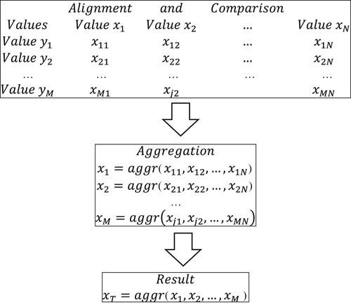
The general framework for ACMA is shown in Figure A.1.
Given two multivalued fields where the first field contains M values and the second field contains N values, the starting point for ACMA is an M×N matrix where each row is labeled by one value of the first multivalued field and each column is labeled by one value of the second multivalued field. Each cell of the M×N matrix is populated with the rating (a number in the interval [0, 1]) that represents the similarity between the corresponding row and column values.
In the first step, the similarity ratings in each row are aggregated into a single similarity rating. In the second step, the aggregated row similarity ratings are aggregated into a final similarity rating. The framework is flexible and can be customized at every step. Customization points include the method for determining the similarity rating between two values, the method of row aggregation, and the method of final aggregation.
For value similarity at the cell level, a single similarity function can be used such as the normalized Levenshtein Edit Distance. Comparators are typically applied after some standardization of the values has been applied, such as removal of punctuation, upper casing, and standard spacing. Instead of one comparator, the framework allows for several comparators to be used to calculate one cell rating. For example, Jaro-Winkler and Maximum q-Gram, which each produce a similarity rating. Reducing multiple ratings to a single cell rating provides another degree of freedom as to how these ratings will be combined – for example, maximum rating, average, or root mean square (RMS) of the ratings.
The simplest form of aggregation is to simply compute the average of all of the similarity ratings, i.e.
An alternate strategy that often works better when M≠N is to calculate the overall rating as the average of the row-column maxima. This is an iterative process starting with the largest cell rating, then the next largest cell rating not in the same row or column of the first rating, then the next largest cell rating not in the same row or column of either of the previous two ratings, and so on. If M≥N, then the iteration will produce N cell ratings. Again, the final rating can be calculated as the maximum rating, the average of the N ratings, or the RMS of ratings.
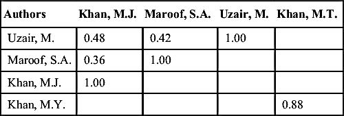
Table A.2 shows a variation of the row-column maxima algorithm comparing author names. To minimize the number of comparisons, the algorithm uses a row-order traversal of the matrix. The algorithm proceeds as follows. Start by assigning the shorter of the two lists of values as row labels. Starting with the first row, calculate the similarity rating for each cell in the row in order. If a rating exceeds a predefined match threshold (e.g. 0.80), stop the comparisons in the row and select that value as the row maximum. Remove the column of the row maximum from further consideration. Go to the next row and follow the same procedure, but do not make any comparisons in columns previously removed from consideration.
In Table A.2, three comparisons were made before reaching the 0.80 threshold. This removes Row 1 and Column 3 from further consideration. In Row 2, the process stops at Column 2, and in Row 3 it stops at Column 1. This leaves Column 4 as the only comparison to be made in Row 4. The final rating for the entire matrix is 0.97, the average of row-column maxima of 1.0, 1.0, 1.0, and 0.88.
Alias Comparators
Approximate semantic matching is when the similarity between strings is based upon their linguistic meaning rather than their character structure. For example, in the English language the name “JIM” is well-known and well-understood as an alternate name (nickname) for the name “JAMES”. Most probabilistic matching schemes for names incorporate some type of nickname or alias table to handle these situations. The problem is the mapping of names to nicknames is not one-to-one. For example, the name “HARRY” could be a nickname for the name “HENRY”, the name “HAROLD”, or perhaps not a nickname at all, i.e. the birth name was given as “HARRY”.
Semantic similarity is even more problematic when dealing with business names. For example, the determination that “TOWING AND RECOVERY” represents the same business activity as “WRECKER SERVICE” is difficult to automate. The methods and techniques for making these discoveries fall into the area of research called latent semantic analysis (Deaton, Doan, Schweiger, 2010; Landauer, Foltz, & Laham, 1998).
Phonetic Comparators
Soundex Comparator
One of the first derived match codes schemes is called the Soundex algorithm. It was first patented in 1918 (Odell & Russell, 1918) and was used in the 1930s as a manual process to match records in the Social Security Administration (Herzog et al., 2007). The name Soundex comes from the combination of the words “Sound” and “Indexing” because it attempts to recognize both the syntactic and phonetic similarity between two names. As with most approximate matching, there are many variations resulting from the adaptation of the algorithm to different applications. The algorithm presented here is from Herzog et al. (2007) using the name “Checker”:
1. Capitalize all letters and drop punctuation → CHECKER
2. Remove the letters A, E, I, O, U, H, W, and Y after the first letter → CCKR
3. Keep first letter but replace the other letters by digits according to the coding {B, F, P, V} replace with 1, {C, G, J, K, Q, S, X, Z} replace with 2, {D, T} replace with 3, {L} replace with 4, {M, N} replace with 5, and {R} replace with 6 → C226
4. Replace consecutive sequences of the same digit with a single digit if the letters they represent were originally next to each other in the name or separated by H or W → C26 (because the 22 comes from letters CK that were next to each other)
5. If the result is longer than 4 characters total, drop digits at the end to make it 4 characters long. If the result is less than 4 characters, add zeros at the end to make it 4 characters long → C260
Using this same algorithm the name “John” produces the Soundex match code value J500. By using these match codes as proxies for the attribute values, the name “John Checker” would be matches to any other names that produce the same match codes such as “Jon Cecker”.
..................Content has been hidden....................
You can't read the all page of ebook, please click here login for view all page.