
Introduction to Numerical Methods
The objectives of this chapter are to introduce numerical methods for:
A major scientific use of computers is in finding numerical solutions to mathematical problems which have no analytical solutions (i.e., solutions which may be written down in terms of polynomials and standard mathematical functions). In this chapter we look briefly at some areas where numerical methods have been highly developed, e.g., solving non linear equations, evaluating integrals, and solving differential equations.
14.1 Equations
In this section we consider how to solve equations in one; unknown numerically. The usual way of expressing the problem is to say that we want to solve the equation f(x) = 0, i.e., we want to find its root (or roots). This process is also described as finding the zeros of f(x). There is no general method for finding roots analytically for an arbitrary f(x).
14.1.1 Newton’s method
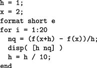
Newton’s method is perhaps the easiest numerical method to implement for solving equations, and was introduced briefly in earlier chapters. It is an iterative method, meaning that it repeatedly attempts to improve an estimate of the root. If xk is an approximation to the root, we can relate it to the next approximation xk+1 using the right-angle triangle in Figure 14.1:
![]()
where f’(x) is df/dx. Solving for xk+1 gives:
![]()
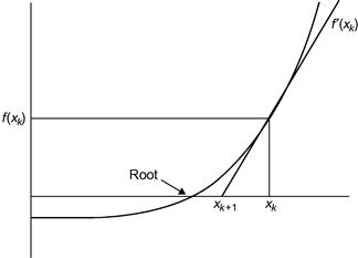
Figure 14.1 Newton’s method.
A structure plan to implement Newton’s method is:
1. Input starting value x0 and required relative error e.
2. While relative error (xk − xk−1)/xk ≥ e repeat up to k = 20, say:
It is necessary to limit step 2 since the process may not converge.
A script using Newton’s method (without the subscript notation) to solve the equation x3 + x − 3 = 0 is given in Chapter 7. If you run it you will see that the values of x converge rapidly to the root.
As an exercise, try running the script with different starting values of x0 to see whether the algorithm always converges.
If you have a sense of history, use Newton’s method to find a root of x3 − 2x − 5 = 0. This is the example used when the algorithm was first presented to the French Academy.
Also try finding a non-zero root of 2x = tan(x), using Newton’s method. You might have some trouble with this one. If you do, you will have discovered the one serious problem with Newton’s method: It converges to a root only if the starting guess is ”close enough.” Since ”close enough” depends on the nature of f(x) and on the root, one can obviously get into difficulties here. The only remedy is some intelligent trial-and-error work on the initial guess—this is made considerably easier by sketching f(x) or plotting it with MATLAB (see Figure 14.2).
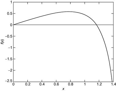
Figure 14.2 f(x) = 2x − tan(x).
If Newton’s method fails to find a root, the Bisection method, discussed below, can be used.
14.1.1.1 Complex roots
Newton’s method can also find complex roots, but only if the starting guess is complex. Use the script in Chapter 10 to find a complex root of x2 + x + 1 = 0. Start with a complex value of 1+i say, for x. Using this starting value for x gives the following output (if you replace disp( [x f(x)] ) in the script with disp( x )):
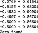
Since complex roots occur in complex conjugate pairs, the other root is −0.5 −0.866i.
14.1.2 The Bisection method
Consider again the problem of solving the equation f(x) = 0, where:
![]()
We attempt to find by inspection, or trial-and-error, two values of x, call them xL and xR, such that f(xL) and f(xR) have different signs, i.e., f(xL)f(xR) < 0. If we can find two such values, the root must lie somewhere in the interval between them, since f(x) changes sign on this interval (see Figure 14.3). In this example, xL = 1 and xR = 2 will do, since f(1) = −1 and f(2) = 7. In the Bisection method, we estimate the root by xM, where xM is the midpoint of the interval [xL, xR], i.e.,
![]() (14.1)
(14.1)
Then if f(xM) has the same sign as f(xL), as drawn in the figure, the root clearly lies between xM and xR. We must then redefine the left-hand end of the interval as having the value of xM, i.e., we let the new value of xL be xM. Otherwise, if f(xM) and f(xL) have different signs, we let the new value of xR be xM, since the root must lie between xL and xM in that case. Having redefined xL or xR, as the case may be, we bisect the new interval again according to Equation (14.1) and repeat the process until the distance between xL and xR is as small as we please.
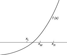
Figure 14.3 The Bisection method.
The neat thing about this method is that, before starting, we can calculate how many Bisections are needed to obtain a certain accuracy, given initial values of xL and xR. Suppose we start with xL = a, and xR = b. After the first Bisection the worst possible error (E1) in xM is E1 = |a − b|/2, since we are estimating the root as being at the midpoint of the interval [a, b]. The worst that can happen is that the root is actually at xL or xR, in which case the error is E1. Carrying on like this, after n Bisections the worst possible error En is given by En = |a − b|/2n. If we want to be sure that this is less than some specified error E, we must see to it that n satisfies the inequality |a − b|/2n < E, i.e.,
![]() (14.2)
(14.2)
Since n is the number of Bisections, it must be an integer. The smallest integer n that exceeds the right-hand side of Inequality (14.2) will do as the maximum number of Bisections required to guarantee the given accuracy E.
The following scheme may be used to program the Bisection method. It will work for any function f(x) that changes sign (in either direction) between the two values a and b, which must be found beforehand by the user.
We have assumed that the procedure will not find the root exactly; the chances of this happening with real variables are infinitesimal.
The main advantage of the Bisection method is that it is guaranteed to find a root if you can find two starting values for xL and xR between which the function changes sign. You can also compute in advance the number of Bisections needed to attain a given accuracy. Compared to Newton’s method it is inefficient. Successive Bisections do not necessarily move closer to the root, as usually happens with Newton’s method. In fact, it is interesting to compare the two methods on the same function to see how many more steps the Bisection method requires than Newton’s method. For example, to solve the equation x3 + x − 3 = 0, the Bisection method takes 21 steps to reach the same accuracy as Newton’s in five steps.
14.1.3 fzero
The MATLAB function fzero(@f, a) finds the zero nearest to the value a of the function f represented by the function f.m.
14.1.4 roots
The MATLAB function M-file roots(c) finds all the roots (zeros) of the polynomial with coefficients in the vector c. See help for details.
Use it to find a zero of x3 + x − 3.
14.2 Integration
Althoughmost “respectable” mathematical functions can be differentiated analytically, the same cannot be said for integration. There are no general rules for integrating, as there are for differentiating. For example, the indefinite integral of a function as simple as e−x2 cannot be found analytically. We therefore need numerical methods for evaluating integrals.
This is actually quite easy, and depends on the fact that the definite integral of a function f(x) between the limits x = a and x = b is equal to the area under f(x) bounded by the x-axis and the two vertical lines x = a and x = b. So all numerical methods for integrating simply involve more or less ingenious ways of estimating the area under f(x).
14.2.1 The Trapezoidal rule
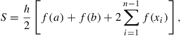
The Trapezoidal (or Trapezium) rule is fairly simple to program. The area under f(x) is divided into vertical panels each of width h, called the step-length. If there are n such panels, then nh = b − a, i.e., n = (b − a)/h. If we join the points where successive panels cut f(x), we can estimate the area under f(x) as the sum of the area of the resulting trapezia (see Figure 14.4). If we call this approximation to the integral S, then:
 (14.3)
where xi = a + ih. Equation (14.3) is the Trapezoidal rule, and provides an estimate for the integral:
![]()
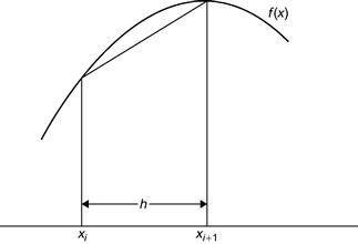
Figure 14.4 The Trapezoidal rule.
Here is a function to implement the Trapezoidal rule:

Note:
1. Since the summation in the rule is implemented with a vectorized formula rather than a for loop (to save time), the function to be integrated must use array operators where appropriate in its M-file implementation.
2. The user must choose h in such a way that the number of steps n will be an integer—a check for this could be built in.
As an exercise, integrate f(x) = x3 between the limits 0 and 4 (remember to write x.ˆ3 in the function M-file). Call trap as follows:
With h = 0.1, the estimate is 64.04, and with h = 0.01 it is 64.0004 (the exact integral is 64). You will find that as h gets smaller, the estimate gets more accurate.
This example assumes that f(x) is a continuous function which may be evaluated at any x. In practice, the function could be defined at discrete points supplied as results of an experiment. For example, the speed of an object v(t) might be measured every so many seconds, and one might want to estimate the distance travelled as the area under the speed-time graph. In this case, trap would have to be changed by replacing fn with a vector of function values. This is left as an exercise for the curious. Alternatively, you can use the MATLAB function interp1 to interpolatethe data. See help.
14.2.2 Simpson’s rule
Simpson’s rule is a method of numerical integration which is a good deal more accurate than the Trapezoidal rule, and should always be used before you try anything fancier. It also divides the area under the function to be integrated, f(x), into vertical strips, but instead of joining the points f(xi) with straight lines, every set of three such successive points is fitted with a parabola. To ensure that there are always an even number of panels, the step-length h is usually chosen so that there are 2n panels, i.e., n = (b − a)/(2h).
Using the same notation as above, Simpson’s rule estimates the integral as:
 (14.4)
Coding this formula into a function M-file is left as an exercise.
If you try Simpson’s rule on f(x) = x3 between any limits, you will find rather surprisingly, that it gives the same result as the exact mathematical solution. This is a nice extra benefit of the rule: it integrates cubic polynomials exactly (which can be proved).
14.2.3 quad
Not surprisingly, MATLAB has a function quad to carry out numerical integration, or quadrature as it is also called. See help.
You may think there is no point in developing our own function files to handle these numerical procedures when MATLAB has its own. If you have got this far, you should be curious enough to want to know how they work, rather than treating them simply as “black boxes.”
14.3 Numerical differentiation
The Newton quotient for a function f(x) is given by:
![]() (14.5)
(14.5)
where h is “small.” As h tends to zero, this quotient approaches the first derivative, df/dx. The Newton quotient may therefore be used to estimate a derivative numerically. It is a useful exercise to do this with a few functions for which you know the derivatives. This way you can see how small you can make h before rounding errorscause problems. Such errors arise because expression (14.5) involves subtracting two terms that eventually become equal when the limit of the computer’s accuracy is reached.
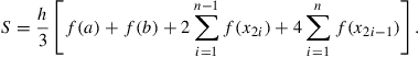
As an example, the following script uses the Newton quotient to estimate f’(x) for f(x) = x2 (which must be supplied as a function file f.m) at x = 2, for smaller and smaller values of h (the exact answer is 4).
Output:
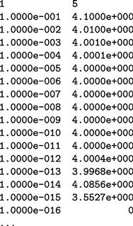
The results show that the best h for this particular problem is about 10−8. But for h much smaller than this the estimate becomes totally unreliable.
Generally, the best h for a given problem can only be found by trial and error. Finding it can be a non-trivial exercise. This problem does not arise with numerical integration, because numbers are added to find the area, not subtracted.
14.3.1 diff
If x is a row or column vector:
then the MATLAB function diff(x) returns a vector of differences between adjacent elements:
The output vector is one element shorter than the input vector.
In certain problems, diff is helpful in finding approximate derivatives, e.g., if x contains displacements of an object every h seconds, diff(x)/h will be its speed.
14.4 First-order differential equations
The most interesting situations in real life that we may want to model, or represent quantitatively, are usually those in which the variables change in time (e.g., biological, electrical or mechanical systems). If the changes are continuous, the system can often be represented with equations involving the derivatives of the dependent variables. Such equations are called differential equations. The main aim of a lot of modeling is to be able to write down a set of differential equations (DEs) that describe the system being studied as accurately as possible. Very few DEs can be solved analytically, so once again, numerical methods are required. We will consider the simplest method of numerical solution in this section: Euler’s method (Euler rhymes with “boiler”). We also consider briefly how to improve it.
14.4.1 Euler’s method
In general we want to solve a first-order DE (strictly an ordinary—ODE) of the form:
![]()
Euler’s method for solving this DE numerically consists of replacing dy/dx with its Newton quotient, so that the DE becomes:
![]()
After a slight rearrangement of terms, we get:
![]() (14.6)
(14.6)
Solving a DE numerically is such an important and common problem in science and engineering that it is worth introducing some general notation at this point. Suppose we want to integrate the DE over the interval x = a (a = 0 usually) to x = b. We break this interval up into m steps of length h, so:
![]()
(this is the same as the notation used in the update process of Chapter 11, except that dt used there has been replaced by the more general h here).
For consistency with MATLAB’s subscript notation, if we define yi as y(xi) (the Euler estimate at the beginning of step i), where xi = (i − 1)h, then yi+1 = y(x + h), at the end of step i. We can then replace Equation (14.6) by the iterative scheme:
![]() (14.7)
(14.7)
where y1 = y(0). Recall from Chapter 11 that this notation enables us to generate a vector y which we can then plot. Note also the striking similarity between Equation (14.7) and the equation in Chapter 11 representing an update process. This similarity is no coincidence. Update processes are typically modeled by DEs, and Euler’s method provides an approximate solution for such DEs.
14.4.2 Example: Bacteria growth
Suppose a colony of 1000 bacteria is multiplying at the rate of r = 0.8 per hour per individual (i.e., an individual produces an average of 0.8 offspring every hour). How many bacteria are there after 10 h? Assuming that the colony grows continuously and without restriction, we can model this growth with the DE:
![]() (14.8)
(14.8)
where N(t) is the population size at time t. This process is called exponential growth. Equation (14.8) may besolved analytically to give the well-known formula for exponential growth:
![]()
To solve Equation (14.8) numerically, we apply Euler’s algorithm to it to get:
![]() (14.9)
(14.9)
where the initial value N1 = 1000.
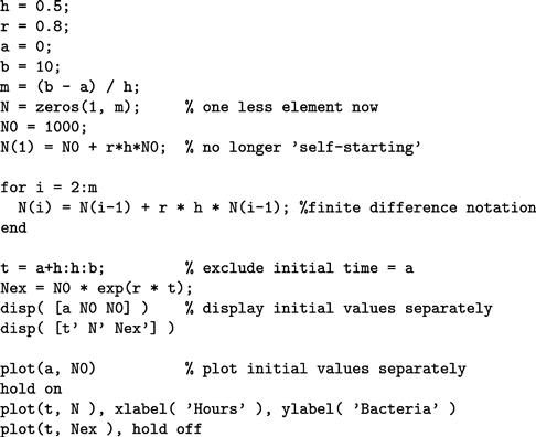
It is very easy to program Euler’s method. The following script implements Equation (14.9), taking h = 0.5. It also computes the exact solution for comparison.
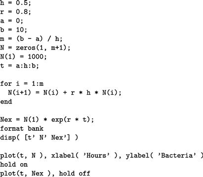
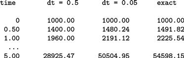
Results are shown in Table 14.1, and also in Figure 14.5. The Euler solution is not too good. In fact, the error gets worse at each step, and after 10 h of bacteria time it is about 72%. The numerical solution will improve if we make h smaller, but there will always be some value of t where the error exceeds some acceptable limit.
Table 14.1
Bacteria growth.
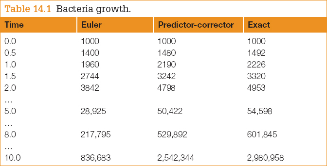
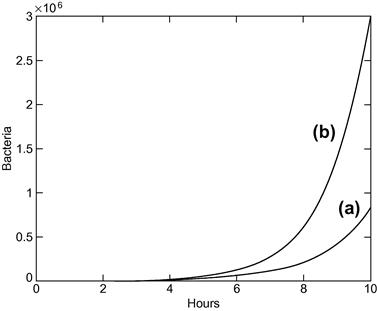
Figure 14.5 Bacteria growth: (a) Euler’s method; (b) the exact solution.
In some cases, Euler’s method performs better than it does here, but there are other numerical methods which always do better than Euler. Two of them are discussed below. More sophisticated methods may be found in most textbooks on numerical analysis. However, Euler’s method may always be used as a first approximation as long as you realize that errors may arise.
14.4.3 Alternative subscript notation
Equation 14.9 is an example of a finite difference scheme. The conventional finite difference notation is for the initial value to be represented by N0, i.e., with subscript i = 0. Ni is then the estimate at the end of step i. If you want the MATLAB subscripts in the Euler solution to be the same as the finite difference subscripts, the initial value N0 must be represented by the MATLAB scalar N0, and you have to compute N(1) separately, before the for loop starts. You also have to display or plot the initial values separately since they will no longer be included in the MATLAB vectors t, N, and Nex (which now have m instead of m + 1 elements). Here is a complete script to generate the Euler solution using finite difference subscripts:
14.4.4 A predictor-corrector method
One improvement on the numerical solution of the first-order DE:
![]()
is as follows. The Euler approximation, which we are going to denote by an asterisk, is given by:
![]() (14.10)
(14.10)
But this formula favors the old value of y in computing f(xi, yi) on the right-hand side. Surely it would be better to say:
![]() (14.11)
(14.11)
where xi+1 = xi + h, since this also involves the new value ![]() in computing f on the right-hand side? The problem of course is that
in computing f on the right-hand side? The problem of course is that ![]() is as yet unknown, so we can’t use it on the right-hand side of Equation (14.11). But we could use Euler to estimate (predict)
is as yet unknown, so we can’t use it on the right-hand side of Equation (14.11). But we could use Euler to estimate (predict) ![]() from Equation (14.10) and then use Equation (14.11) to correct the prediction by computing a better version of
from Equation (14.10) and then use Equation (14.11) to correct the prediction by computing a better version of ![]() , which we will call yi+1. So the full procedure is:
, which we will call yi+1. So the full procedure is:
This is called a predictor-corrector method. The script above can easily be adapted to this problem. The relevant lines of code are:
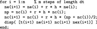
ne stands for the “straight” (uncorrected) Euler solution, np is the Euler predictor (since this is an intermediate result a vector is not needed for np), and nc is the corrector. The worst error is now only 15%. This is much better than the uncorrected Euler solution, although there is still room for improvement.
14.5 Linear ordinary differential equations (LODEs)
Linear ODEs with constant coefficients may be solved analytically in terms of matrix exponentials, which are represented in MATLAB by the function expm. For an example see MATLAB Help: Mathematics: Matrices and Linear Algebra: Matrix Powers and Exponentials.
14.6 Runge-Kutta methods
There are a variety of algorithms, under the general name of Runge-Kutta, which can be used to integrate systems of ODEs. The formulae involved are rather complicated; they can be found in most books on numerical analysis.
However, as you may have guessed, MATLAB has plenty of ODE solvers, which are discussed in MATLAB Help: Mathematics: Differential Equations. Among them are ode23 (second/third order) and ode45 (fourth/fifth order), which implement Runge-Kutta methods. (The order of a numerical method is the power of h (i.e., dt) in the leading error term.) Since h is generally very small, the higher the power, the smaller the error. We will demonstrate the use of ode23 and ode45 here, first with a single first-order DE, and then with systems of such equations.
14.6.1 A single differential equation
Here’s how to use ode23 to solve the bacteria growth problem, Equation (14.8):
![]()
1. Start by writing a function file for the right-hand side of the DE to be solved. The function must have input variables t and N in this case (i.e., independent and dependent variables of the DE), in that order, e.g., create the function file f.m as follows:
2. Now enter the following statements in the Command Window:
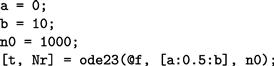
3. Note the input arguments of ode23:
@f: a handle for the function f, which contains the right-hand side of the DE;
[a:0.5:b]: a vector (tspan) specifying the range of integration. If tspan has two elements ([a b]) the solver returns the solution evaluated at every integration step (the solver chooses the integration steps and may vary them). This form would be suitable for plotting. However, if you want to display the solution at regular time intervals, as we want to here, use the form of tspan with three elements as above. The solution is then returned evaluated at each time in tspan. The accuracy of the solution is not affected by the form of tspan used.
n0: the initial value of the solution N.
4. The output arguments are two vectors: the solutions Nr at times t. For 10 h ode23 gives a value of 2,961,338 bacteria. From the exact solution in Table 14.1 we see that the error here is only 0.7%.
If the solutions you get from ode23 are not accurate enough, you can request greater accuracy with an additional optional argument. See help.
If you need still more accurate numerical solutions, you can use ode45 instead. It gives a final value for the bacteria of 2981290—an error of about 0.01%.
14.6.2 Systems of differential equations: Chaos
The reason that weather prediction is so difficult and forecasts are so erratic is no longer thought to be the complexity of the system but the nature of the DEs modeling it. These DEs belong to a class referred to as chaotic. Such equations will produce wildly different results when their initial conditions are changed infinitesimally. In other words, accurate weather prediction depends crucially on the accuracy of the measurements of the initial conditions:
Edward Lorenz, a research meteorologist, discovered this phenomenon in 1961. Although his original equations are far too complex to consider here, the following much simpler system has the same essential chaotic features:
![]() (14.12)
(14.12)
![]() (14.13)
(14.13)
![]() (14.14)
(14.14)
This system of DEs may be solved very easily with the MATLAB ODE solvers. The idea is to solve the DEs with certain initial conditions, plot the solution, then change the initial conditions very slightly, and superimpose the new solution over the old one to see how much it has changed.
We begin by solving the system with the initial conditions x(0) = −2, y(0) = −3.5, and z(0) = 21.
1. Write a function file lorenz.m to represent the right-hand sides of the system as follows:
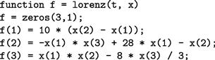
The three elements of the MATLAB vector x, i.e., x(1), x(2), and x(3), represent the three dependent scalar variables x, y, and z respectively. The elements of the vector f represent the right-hand sides of the three DEs. When a vector is returned by such a DE function it must be a column vector, hence the statement,
2. Now use the following commands to solve the system from t = 0 to t = 10, say:
![]()
Note that we are use ode45 now, since it is more accurate. You will see three graphs, for x, y, and z (in different colors).
3. It’s easier to see the effect of changing the initial values if there is only one graph in the figure to start with. It is in fact best to plot the solution y(t) on its own. The MATLAB solution x is actually a matrix with three columns (as you can see from whos). The solution y(t) that we want will be the second column, so to plot it by itself use the command:
Then keep the graph on the axes with the command hold.
Now we can see the effect of changing the initial values. Let’s just change the initial value of x(0), from −2 to −2.04—that’s a change of only 2%, and in only one of the three initial values. The following commands will do this, solve the DEs, and plot the new graph of y(t) (in a different color):
![]()
You should see (Figure 14.6) that the two graphs are practically indistinguishable until t is about 1.5. The discrepancy grows quite gradually, until t reaches about 6, when the solutions suddenly and shockingly flip over in opposite directions. As t increases further, the new solution bears no resemblance to the old one.
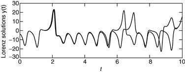
Figure 14.6 Chaos?
Now solve the system (14.12–14.14) with the original initial values using ode23 this time:
Plot the graph of y(t) only—x(:,2)—and then superimpose the ode45 solution with the same initial values (in a different color).
A strange thing happens—the solutions begin to deviate wildly for t > 1.5! The initial conditions are the same—the only difference is the order of the Runge-Kutta method.
Finally solve the system with ode23s and superimpose the solution. (The s stands for “stiff” For a stiff DE, solutions can change on a time scale that is very short compared to the interval of integration.) The ode45 and ode23s solutions only start to diverge at t > 5.
The explanation is that ode23, ode23s, and ode45 all have numerical inaccuracies (if one could compare them with the exact solution—which incidentally can’t be found). However, the numerical inaccuracies are different in the three cases. This difference has the same effect as starting the numerical solution with very slightly different initial values.
How do we ever know when we have the “right” numerical solution? Well, we don’t—the best we can do is increase the accuracy of the numerical method until no further wild changes occur over the interval of interest. So in our example we can only be pretty sure of the solution for t < 5 (using ode23s or ode45). If that’s not good enough, you have to find a more accurate DE solver.
So beware: “chaotic” DEs are very tricky to solve!
Incidentally, if you want to see the famous “butterfly” picture of chaos, just plot x against z as time increases (the resulting graph is called a a phase plane plot). The following command will do the trick:
What you will see is a static 2-D projection of the trajectory, i.e., the solution developing in time. Demos in the MATLAB Launch Pad include an example which enables you to see the trajectory evolving dynamically in 3-D (Demos: Graphics: Lorenz attractor animation).
14.6.3 Passing additional parameters to an ODE solver
In the above examples of the MATLAB ODE solvers the coefficients in the right-hand sides of the DEs (e.g., the value 28 in Equation (14.13)) have all been constants. In a real modeling situation, you will most likely want to change such coefficients frequently. To avoid having to edit the function files each time you want to change a coefficient, you can pass the coefficients as additional parameters to the ODE solver, which in turn passes them to the DE function. To see how this may be done, consider the Lotka-Volterra predator-prey model:
![]() (14.15)
(14.15)
![]() (14.16)
(14.16)
where x(t) and y(t) are the prey and predator population sizes at time t, and p, q, r and s are biologically determined parameters. For this example, we take p = 0.4, q = 0.04, r = 0.02, s = 2, x(0) = 105, and y(0) = 8.
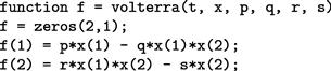
First, write a function M-file, volterra.m as follows:
Then enter the following statements in the Command Window, which generate the characteristically oscillating graphs in Figure 14.7:
![]()
Note:
![]() The additional parameters (p, q, r, and s) have to follow the fourth input argument (options—see help) of the ODE solver. If no options have been set (as in our case), use [ ] as a placeholder for the options parameter.
The additional parameters (p, q, r, and s) have to follow the fourth input argument (options—see help) of the ODE solver. If no options have been set (as in our case), use [ ] as a placeholder for the options parameter.
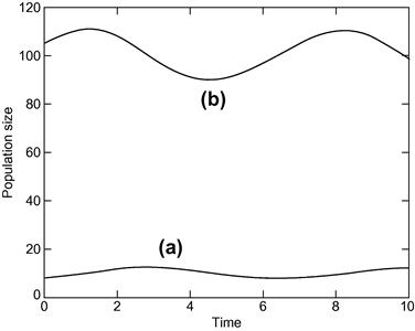
Figure 14.7 Lotka-Volterra model: (a) predator; (b) prey.
You can now change the coefficients from the Command Window and get a new solution, without editing the function file.
14.7 A partial differential equation
The numerical solution of partial differential equations (PDEs) is a vast subject, which is beyond the scope of this book. However, a class of PDEs called parabolic often lead to solutions in terms of sparse matrices, which were mentioned briefly in Chapter 16. One such example is considered in this section.
14.7.1 Heat conduction
The conduction of heat along a thin uniform rod may be modeled by the partial differential equation:
![]() (14.17)
(14.17)
where u(x,t) is the temperature distribution a distance x from one end of the rod at time t, and assuming that no heat is lost from the rod along its length.
Half the battle in solving PDEs is mastering the notation. We set up a rectangular grid, with step-lengths of h and k in the x and t directions respectively. Ageneral point on the grid has co-ordinates ![]() . A concise notation for u(x,t) at xi, yj is then simply ui, j.
. A concise notation for u(x,t) at xi, yj is then simply ui, j.
Truncated Taylor series may then be used to approximate the PDE by a finite difference scheme. The left-hand side of Equation (14.17) is usually approximated by a forward difference:
![]()
One way of approximating the right-hand side of Equation (14.17) is by the scheme:
![]() (14.18)
(14.18)
This leads to a scheme, which although easy to compute, is only conditionally stable.
If however we replace the right-hand side of the scheme in Equation (14.18) by the mean of the finite difference approximation on the jth and (j + 1)th time rows, we get (after a certain amount of algebra!) the following scheme for Equation (14.17):
![]() (14.19)
(14.19)
where r = k/h2. This is known as the Crank-Nicolson implicit method, since it involves the solution of a system of simultaneous equations, as we shall see.
To illustrate the method numerically, let’s suppose that the rod has a length of 1 unit, and that its ends are in contact with blocks of ice, i.e., the boundary conditions are:
![]() (14.20)
(14.20)
Suppose also that the initial temperature (initial condition) is:
![]() (14.21)
(14.21)
(This situation could come about by heating the center of the rod for a long time, with the ends kept in contact with the ice, removing the heat source at time t = 0.) This particular problem has symmetry about the line x = 1/2; we exploit this now in finding the solution.
If we take h = 0.1 and k = 0.01, we will have r = 1, and Equation (14.19) becomes:
![]() (14.22)
(14.22)
Putting j = 0 in Equation (14.22) generates the following set of equations for the unknowns ui,1 (i.e., after one time step k) up to the midpoint of the rod, which is represented by i = 5, i.e., x = ih = 0.5. The subscript j = 1 has been dropped for clarity:
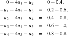
Symmetry then allows us to replace u6 in the last equation by u6. These equations can be written in matrix form as:
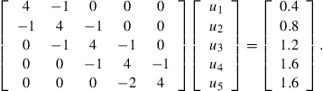 (14.23)
The matrix (A) on the left of Equations (14.23) is known as a tridiagonal matrix. Having solved for the ui,1 we can then put j = 1 in Equation (14.22) and proceed to solve for the ui,2, and so on. The system (14.23) can of course be solved directly in MATLAB with the left division operator. In the script below, the general form of Equations (14.23) is taken as:
![]() (14.24)
(14.24)
Care needs to be taken when constructing the matrix A. The following notation is often used:
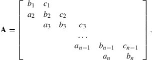
A is an example of a sparse matrix (see Chapter 16).
The script below implements the general Crank-Nicolson scheme of Equation (14.19) to solve this particular problem over 10 time steps of k = 0.01. The step-length is specified by h = 1/(2n) because of symmetry. r is therefore not restricted to the value 1, although it takes this value here. The script exploits the sparsity of A by using the sparse function.
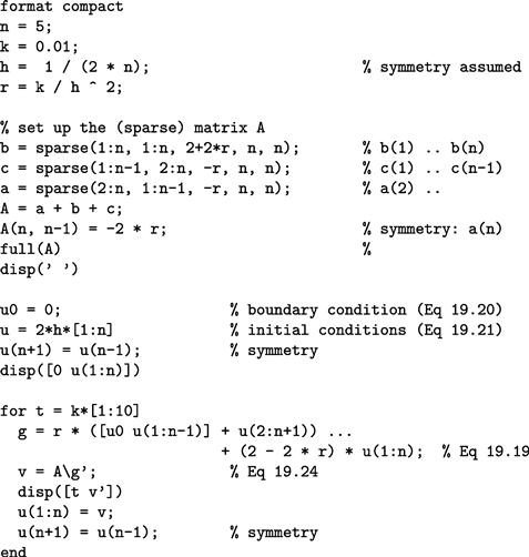
Note:
![]() To preserve consistency between the formal subscripts of Equation (14.19) etc. and MATLAB subscripts, u0 (the boundary value) is represented by the scalar u0.
To preserve consistency between the formal subscripts of Equation (14.19) etc. and MATLAB subscripts, u0 (the boundary value) is represented by the scalar u0.
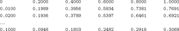
In the following output the first column is time, and subsequent columns are the solutions at intervals of h along the rod:
MATLAB has some built-in PDE solvers. See MATLAB Help: Mathematics: Differential Equations: Partial Differential Equations.
14.8 Other numerical methods
The ODEs considered earlier in this chapter are all initial value problems. For boundary value problem solvers, see MATLAB Help: Mathematics: Differential Equations: Boundary Value Problems for ODEs.
MATLAB has a large number of functions for handling other numerical procedures, such as curve fitting, correlation, interpolation, minimization, filtering and convolution, and (fast) Fourier transforms. Consult MATLAB Help: Mathematics: Polynomials and Interpolation and Data Analysis and Statistics.
Here’s an example of curve fitting. The following script enables you to plot data points interactively. When you have finished plotting points (signified when the x coordinates of your last two points differ by less than two in absolute value) a cubic polynomial is fitted and drawn (see Figure 14.8).
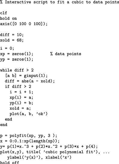
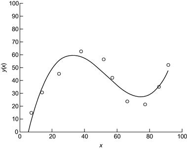
Figure 14.8 A cubic polynomial fit.
Polynomial fitting may also be done interactively in a figure window, with Tools -> Basic Fitting.
Summary
![]() A numerical method is an approximate computer method for solving a mathematical problem which often has no analytical solution.
A numerical method is an approximate computer method for solving a mathematical problem which often has no analytical solution.
![]() A numerical method is subject to two distinct types of error: Rounding error in the computer solution, and truncation error, where an infinite mathematical process, like taking a limit, is approximated by a finite process.
A numerical method is subject to two distinct types of error: Rounding error in the computer solution, and truncation error, where an infinite mathematical process, like taking a limit, is approximated by a finite process.
![]() MATLAB has a large number of useful functions for handling numerical methods.
MATLAB has a large number of useful functions for handling numerical methods.
Chapter exercises
14.1 Use Newton’s method in a script to solve the following (you may have to experiment a bit with the starting values). Check all your answers with fzero. Check the answers involving polynomial equations with roots. Hint: use fplot to get an idea of where the roots are, e.g.,
fplot(‘x^3-8*x^ 2+17* x-10’, [0 3])
The Zoom feature also helps. In the figure window select the Zoom In button (magnifying glass) and click on the part of the graph you want to magnify.
(a) ![]() (two real roots and two complex roots).
(two real roots and two complex roots).
(c) x3 − 8x2 + 17x − 10 = 0 (three real roots).
(e) x4 − 5x3 − 12x2 + 76x − 79 = 0 (four real roots).
14.2 Use the Bisection method to find the square root of 2, taking 1 and 2 as initial values of xL and xR. Continue bisecting until the maximum error is less than 0.05 (use Inequality (14.2) of Section 14.1 to determine how many Bisections are needed).
14.3 Use the Trapezoidal rule to evaluate ![]() , using a step-length of h = 1.
, using a step-length of h = 1.
14.4 A human population of 1000 at time t = 0 grows at a rate given by
![]()
where a = 0.025 per person per year. Use Euler’s method to project the population over the next 30 years, working in steps of (a) h = 2 years, (b) h = 1 year, and (c) h = 0.5 years. Compare your answers with the exact mathematical solution.
14.5 Write a function file euler.m which starts with the line:
function [t, n] = euler(a, b, dt)
and which uses Euler’s method to solve the bacteria growth DE (14.8). Use it in a script to compare the Euler solutions for dt = 0.5 and 0.05 with the exact solution. Try to get your output looking like this:
14.6 The basic equation for modeling radio-active decay is:
![]()
where x is the amount of the radio-active substance at time t, and r is the decay rate.
Some radio-active substances decay into other radio-active substances, which in turn also decay. For example, Strontium 92 (r1 = 0.256/h) decays into Yttrium 92 (r2 = 0.127/h), which in turn decays into Zirconium. Write down a pair of differential equations for Strontium and Yttrium to describe what is happening.
Starting at t = 0 with 5 × 1026 atoms of Strontium 92 and none of Yttrium, use the Runge–Kutta method (ode23) to solve the equations up to t = 8 h in steps of 1/3 h. Also use Euler’s method for the same problem, and compare your results.
14.7 The springbok (a species of small buck, not rugby players!) population x(t) in the Kruger National Park in South Africa may be modeled by the equation:
![]()
where r, b, and a are constants. Write a program which reads values for r, b, and a, and initial values for x and t, and which uses Euler’s method to compute the impala population at monthly intervals over a period of two years.
14.8 The luminous efficiency (ratio of the energy in the visible spectrum to the total energy) of a black body radiator may be expressed as a percentage by the formula:
![]()
where T is the absolute temperature in degrees Kelvin, x is the wavelength in cm, and the range of integration is over the visible spectrum.
Write a general function simp(fn, a, b, h) to implement Simpson’s rule as given in Equation (14.4).
Taking T = 3500°K, use simp to compute E, firstly with 10 intervals (n = 5), and then with 20 intervals (n = 10), and compare your results.(Answers: 14.512725% for n = 5; 14.512667% for n = 10)
14.9 Van der Pol’s equation is a second-order non-lineardifferential equation which may be expressed as two first-order equations as follows:
![]()
The solution of this system has a stable limit cycle, which means that if you plot the phase trajectory of the solution (the plot of x1 against x2) starting at any point in the positive x1 − x2 plane, it always moves continuously into the same closed loop. Use ode23 to solve this system numerically, for x1(0) = 0, and x2(0) = 1. Draw some phase trajectories for b = 1 and ɛ ranging between 0.01 and 1.0. Figure 14.9 shows you what to expect.
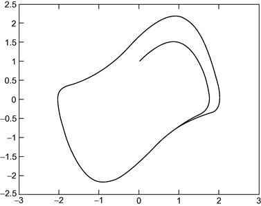
Figure 14.9 A trajectory of Van der Pol’s equation.