Data for AI

At the core of many popular machine learning models, including the highly successful neural networks that brought Artificial Intelligence back into popular spotlight since AlexNet in 2012, lies a very simple mathematical problem:

Fit a given set of data points into an appropriate function, that picks up on the important signals in the data and ignores the noise, then make sure this function performs well on new data.

Complexity and challenges, however, arise from various sources:

Hypothesis and features

Neither the true function that generated the data nor all the features it actually depends on are known. We simply observe the data then try to estimate a hypothetical function that generated it. Our function tries to learn which features of the data are important for our predictions, classifications, decisions, or general purposes. It also learns how these features interact in order to produce the observed results. One of the great potential of AI in this context is its ability to pick up on subtle interactions between features of data that humans do not usually pick up on, since we are very good at observing strong features but ignoring more subtle ones. For example, we as humans can tell that a person’s monthly income affects their ability to pay back a loan, but we might not observe that their daily commute, or morning routine, might have a nontrivial effect on that as well. Some feature interactions are much simpler than others, such as linear interactions. Others are more complex, and are nonlinear. From a mathematical point of view, whether our feature interactions are simple (linear) or complex (nonlinear), we still have the same goal: Find the hypothetical function that fits your data and is able to make good predictions on new data. One extra complication arises here: There are many hypothetical functions that can fit the same data set, how do we know which ones to choose?

Performance

Even after computing a hypothetical function that fits our data, how do we know whether it will perform well on new and unseen data? How do we know which performance measure to choose, and how to monitor this performance after deploying into the real world? Real world data and scenarios do not come to us all labeled with ground truths, so we cannot easily measure whether our AI system is doing well and making correct or appropriate predictions and decisions. We do not know what to measure the AI system’s results against. If real world data and scenarios were labeled with ground truths, then we would all be out of business since we would know what to do in every situation, there would be peace on Earth, and we would live happily ever after.

Volume

Almost everything in the AI field is very high dimensional! The number of data instances, observed features, and unknown weights to be computed could be in the millions, and the required computation steps in the billions. Efficient storage, transport, exploration, preprocessing, structuring, and computation on such volumes of data become centerfold goals. In addition, exploring the landscapes of the involved high dimensional mathematical functions is a nontrivial endeavor.

Structure

The vast majority of data created by the modern world is unstructured. It is not organized in easy to query tables that contain labeled fields such as names, phone numbers, gender, age, zip codes, house prices, income level, etc. Unstructured data is everywhere: Posts on social media, user activity, word documents, pdf files, images, audio and video files, collaboration software data, traffic, seismic, and weather data, GPS, military movement, emails, instant messenger, mobile chat data, and many others. Some of these examples, such as email data, can be considered semi-structured, since emails come with headings that include the email’s metadata: From, To, Date, Time, Subject, Content-Type, Spam Status, etc. Moreover, large volumes of important data are not available in digital format and are fragmented over multiple and non-communicating data bases. Examples here include historical military data, museums, and hospital records. Presently, there is great momentum towards digitalizing our world and our cities, in order to leverage more AI applications. Overall, it is easier to draw insights from structured and labeled data than unstructured data. Mining unstructured data requires innovative techniques that are currently driving forces in the fields of data science, machine learning, and artificial intelligence.

Real Data vs. Simulated Data

When we work with data, it is very important to know the difference between real data and simulated data. Both types of data are extremely valuable for human discovery and progress.

Real data

This data is collected through real world observations, using measuring devices, sensors, surveys, structured forms like medical questionnaires, telescopes, imaging devices, websites, stock markets, controlled experiments, etc. This data is often imperfect and noisy, due to inaccuracies and failures in measuring methods and instruments. Mathematically, we do not know the exact function or probability distribution that generated the real data but we can hypothesize about them using models, theories, and simulations. We can then test our models, and finally use them to make predictions.

Simulated data

This is data generated using a known function or randomly sampled from a known probability distribution. Here, we have our known mathematical function(s), or model, and we plug numerical values into the model inorder to generate our data points. Examples are unnumerable: Disney movie animations (Frozen, Moana, etc.), numerical solutions of partial differential equations modeling all kinds of natural phenomena, on all kinds of scales, such as turbulent flows, protein folding, heat diffusion, chemical reactions, planetary motion, fractured materials, traffic, etc.

In this chapter, we present two examples about human height and weight data in order to demonstrate the difference between real and simulated data. In the first example, we visit an online public database, then download and explore two real data sets containing measurements of the heights and weights of real individuals. In the second example, we simulate our own data set of heights and weights based on a function that we hypothesize: We assume that the weight of an individual depends linearly on their height, meaning that when we plot the weight data against the height data, we expect to see a straight, or flat, visual pattern.

Mathematical Models: Linear vs. Nonlinear

Linear dependencies model flatness in the world, like one dimensional straight-lines, two dimensional flat surfaces (called planes), and higher dimensional hyper-planes. The graph of a linear function, which models a linear dependency, is forever flat and does not bend. Every time you see a flat object, like a table, a rod, a ceiling, or a bunch of data points huddled together around a straight-line or a flat surface, know that their representative function is linear. Anything other than flat is nonlinear, so functions whose graphs bend are nonlinear, and data points which congregate around bending curves or surfaces must have been generated by nonlinear functions.

The formula for a linear function, representing a linear dependency of the function output on the features, or variables, is very easy to write down. The features appear in the formula as just themselves, with no powers or roots, and are not embedded in any other functions, such as denominators of fractions, sine, cosine, exponential, logarithmic or other calculus functions. They can only be multiplied by scalars, and added or subtracted to and from each other. For example, a function that depends linearly on three features $x_1,x_2$ and $x_3$ can be written as:

where the parameters ${\omega }_0,{\omega }_1,{\omega }_2$ and ${\omega }_3$ are scalar numbers. The parameters, or weights ${\omega }_1,{\omega }_2$, and ${\omega }_3$ linearly combine the features, and produce the outcome of $f(x_1,x_2,x_3)$ after adding the bias term ${\omega }_0$. In other words, the outcome is produced as a result of linear interactions between the features $x_1,x_2$ and $x_3$, plus bias.

The formula for a nonlinear function, representing a nonlinear dependency of the function output on the features, is very easy to spot as well: One or more features appear in the function formula with a power other than one, or multiplied or divided by other features, or embedded in some other calculus functions, such as sines, cosines, exponentials, logarithms, etc. The following are three examples of functions depending nonlinearly on three features $x_1,x_2$ and $x_3$:

As you can tell, we can come up with all kinds of nonlinear functions, and the possibilities related to what we can do and how much of the world we can model using nonlinear interactions are limitless. In fact, neural networks are successful because of their ability to pick up on the relevant nonlinear interactions between the features of the data.

We will use the above notation and terminology throughout the book, so you will become very familiar with terms like linear combination, weights, features, and linear and nonlinear interactions between features.

An Example of Real Data

You can find the python code to investigate the data and produce the figures in the following two examples at the linked Jupyter notebook for Chapter 2.

I downloaded two data sets from Kaggle website for data scientists. Both data sets contain height, weight and gender information for a certain number of individuals. My goal is to learn how the weight of a person depends on their height. Mahematically, I want to write a formula for the weight as a function of one feature, the height:

so that if I am given the height of a new person, I would be able to predict their weight. Of course, there are other features than height that a person’s weight depends on, such as their gender, eating habits, workout habits, genetic predisposition, etc.. However, for the data sets that I downloaded, we only have height, weight, and gender data available. Unless we want to look for more detailed data sets, or go out and collect new data, we have to work with what we have. Moreover, the goal of this example is only to illustrate the difference between real data and simulated data. We will be working with more involved data sets with larger number of features when we have more involved goals.

For the first data set, I plot the weight column against the height column in Figure 2-1, and obtain something that seems to have no pattern at all!

Figure 2-1. When plotting the weight against the height for the first data set, we cannot detect a pattern.

For the second data set, I do the same, and I can visually observe an obvious linear dependency in Figure 2-2. The data points seem to congregate around a straight-line!

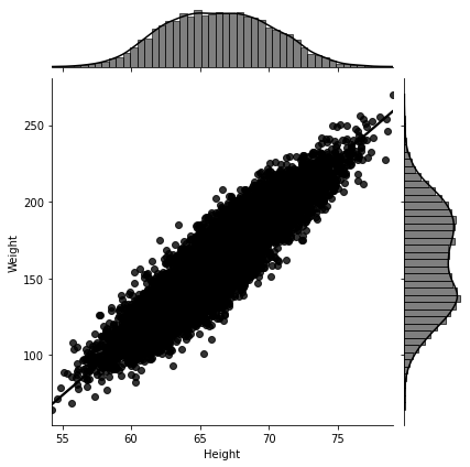
Figure 2-2. When plotting the weight against the height for the second data set, we observe a linear pattern. Note that the distribution of the weight data is plotted on the right hand side of the figure, and the distribution of the height data is plotted on the top of the figure. Both seem to have two peaks (bimodal), suggesting the existence of a mixture distribution. In fact, both the height and weight data sets can be modeled using a mixture of two normal distributions, called Gaussian mixtures, representing mixing the underlying distributions for the male and female data. So if we plot the data for either the female or male subpopulations alone, as in Figure 2-6, we observe that the height and weight data are normally distributed (bell shaped).

So what is going on? Why does my first real data set reflect no dependency between the height and weight of a person whatsoever, but my second one reflects a linear dependency? We need to investigate deeper into the data.

This is one of the many challenges of working with real data. We do not know what function generated the data, and why it looks the way it looks. We investigate, gain insights, detect patterns, if any, and we propose a hypothesis function. Then we test our hypothesis, and if it performs well based on our measures of performance, which have to be thoughtfully crafted, we deploy it into the real world. We make predictions using our deployed model, until new data tells us that our hypothesis is no longer valid, in which case, we investigate the updated data, and formulate a new hypothesis. This process keeps going.

Before moving on to simulated data, let’s explain why the first data set seemed to have no insight at all about the relationship between the height and the weight of an individual. Upon further inspection, we notice that the data set has an overrepresenation of individuals with Index scores 4 and 5, referring to Obesity and Extreme Obesity. So, I decided to split the data by Index score, and plot the weight against the height for all individuals with similar Index scores. This time around, a linear dependency between the height and the weight is evident in Figure 2-3, and the mystery is resolved. The following figure shows the weight against the height for individuals with Index score 3.

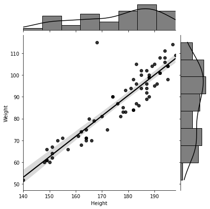
Figure 2-3. When plotting the weight against the height for individuals with similar Index score in the the first data set, we observe a linear pattern.

Now we can safely go ahead and hypothesize that the weight depends linearly on the height:

Of course, we are left with the task of finding appropriate values for the parameters ${\omega }_0$ and ${\omega }_1$. The next chapter teaches us how to do exactly that. In fact, the bulk of activity in machine learning, including deep learning, is about learning these $\omega$’s from the data. In our very simple example, we only have two $\omega$’s to learn, since we only had one feature, the height, and we assumed linear dependency, after observing a linear pattern in the real data. In the next few chapters, we will encounter some deep learning networks with millions of $\omega$’s to learn, yet, we will see that the mathematical structure of the problem is in fact similar to the same structure that will be presented in Chapter 3.

An Example of Simulated Data

In this example, I simulate my own Height Weight data set. Simulating our own data circumvents the trouble of searching for data from the web, the real world, or even building a lab in order to obtain controlled measurements. This is incredibly valuable when the required data is not available, or very expensive to obtain. It also helps test different scenarios by only changing numbers in a function, as opposed to say, creating new materials, or building labs, and running new experiments. Simulating data is so convenient because all we need is a mathematical function, a probability distribution if we want to involve randomness and/or noise, and a computer.

Let’s again assume linear dependency between the height and the weight, so the function that we will use is:

For us to be able to simulate numerical $(height,weight)$ pairs, or data points, we must assume numerical values for the parameters ${\omega }_0$ and ${\omega }_1$. Without having insights from real data about the correct choices for these $\omega$’s, we are left with making educated guesses from the context of the problem and experimenting with different values. Note that for the Height Weight case in this example, we happen to have real data that we can use to learn appropriate values for the $\omega$’s, and one of the goals of Chapter 3 is to learn how to do that. However, in many other scenarios, we do not have real data, so the only way to go is experimenting with various numerical values for these $\omega$’s.

In the following simulations, we set ${\omega }_0=-314.5$ and ${\omega }_1=7.07$, so the function becomes:

Now we can generate as many numerical $(height,weight)$ pairs as we want. For example, plugging $height=60$ in the formula for the weight function, we get $weight=-314.5+7.07\times 60=109.7$. So our linear model predicts that a person whose height is 60 inches weighs $109.7$ lbs, and the data point that we can plot on the Height Weight graph has coordinates $(60,109.7)$. In Figure 2-4, we generate 5000 of these data points: We choose 5000 values for the height between 54 and 79 inches and plug them into the weight function. We notice that the graph in Figure 2-4 is a perfect straight-line, with no noise or variation in the simulated data, since I did not incorporate those into my linear model. That’s a hallmark of simulated data: It does what the function(s) it was generated from does. If we understand the function (called model) that we used to build our simulation, and if our computation does not accumulate too many numerical errors and/or very large numbers that go rogue, then we understand the data that our model generates, and we can use this data in any way we see fit. There isn’t much space for surprises. In our example, our proposed function is linear, so its equation is that of a straight-line, and as you see in Figure 2-4, the generated data lies perfectly on this straight-line.

Figure 2-4. Simulated data: We generated five thousand (height, weight) points using the linear function $weight=-314.5+7.07\times height$.

What if we want to simulate more realistic data for height and weight? Then we can sample the height values from a more realistic distribution for the heights of a human population: The bell shaped normal distribution! Again, we know the probability distribution that we are sampling from, which is different from the case for real data. After we sample the height values, we plug those into the linear model for the weight, then we add some noise, since we want our simulated data to be realistic. Since noise has a random nature then we must also pick the probability distribution it will be sampled from. We again choose the bell shaped normal distribution, but we could’ve chosen the uniform distribution to model uniform random fluctuations. Our more realistic Height Weight model becomes:

We obtain Figure 2-5.

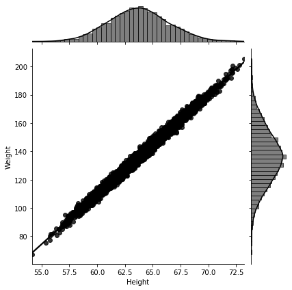
Figure 2-5. Simulated data: We generated five thousand (height, weight) points using the linear function $weight=-314.5+7.07\times height$. The height points are normally distributed and we added normally distributed noise as well. Note that the distributions of the weight and height data at the right hand side and at the top of the figure respectively are normally distributed. This is not surprising since we designed them that way in our simulation.

Now compare Figure 2-5 containing our simulated Height Weight data to Figure 2-6 containing real Height Weight data of 5000 females from the second Kaggle data set that we used. Not too bad, given that it only took five minutes of code writing to generate this data, as opposed to collecting real data! Had we spent more time tweaking the values of our $\omega$’s, and the parameters for the normally distributed noise that we added (mean and standard deviation), we would’ve obtained an even better looking simulated data set. However, we will leave this simulation here since very soon our whole focus will be on learning the appropriate parameter values for our hypothesized models.

Figure 2-6. Real Data: Weight data plotted against the height data of the 5000 females in the second Kaggle data set. Note that the distributions of the female weight and height data at the right hand side and at the top of the figure respectively are normally distributed. Check the linked Jupyter Notebook for more details.

Mathematical Models: Simulations and AI

We can always adjust our mathematical models to make them more realistic. We are the designers so we get to decide what goes into these models. It is often the case that the more a model mimics nature the more mathematical objects get incorporated within it. Therefore, while building a mathematical model, the usual tradeoff is between getting closer to reality, and the model’s simplicity and accessibility for mathematical analysis and computation. Different designers come up with different mathematical models, and some capture certain phenomena better than others. These models keep improving and evolving as the quest to capture natural behaviors continues. Thankfully, our computational capabilities have dramatically improved in the past decades, enabling us to create and test more involved and realistic mathematical models.

Nature is at the same time very finely detailed and enormously vast. Interactions in nature range from the subatomic quantum realm all the way to intergalactic interactions. We, as humans, are forever trying to undertsand nature and capture its intricate components with their numerous interconnections and interplays. Our reasons for this are varied. They range from pure curiosity about the origins of life and the universe, to creating new technologies, to building weapons, to enhancing communication systems, to designing drugs and discovering cures for diseases, to traveling to distant planets and perhaps inhabiting them in the future. Mathematical models provide an excellent and almost miraculous way to describe nature with all its details using only numbers, functions, equations, and invoking quantified randomness through probability when faced with uncertainty. Computer simulations of these mathematical models enable us to investigate and visualize various simple and complex behaviors of the modeled systems or phenomena. In turn, insights from computer simulations aid in model enhancement and design, in addition to supplying deeper mathematical insights. This incredibly positive feedback cycle makes mathematical modeling and simulations an indespensible tool that is enhanced greatly with our increased computational power.

It is a mystery of the universe that its various phenomena can be accurately modeled using the abstract language of mathematics, and it is a marvel of the human mind that it can discover and comprehend mathematics, and build powerful technological devices that are useful for all kinds of applications. Equally impressive is that these devices, at their core, are doing nothing but computing or transmitting mathematics, more specifically, a bunch of zeros and ones.

The fact that humans are able to generalize their understanding of simple numbers all the way to building and applying mathematical models for natural phenomena at all kinds of scales is a spectacular example of generalization of learned knowledge, and is a hallmark of human’s intelligence. In the AI field, a common goal for both general AI and narrow AI is generalization: The ability of an AI agent to generalize learned abilities to new and unknown situations. In the next chapter, we will understand this principle for narrow and task oriented AI: An AI agent learns from data then produces good predictions for new and unseen data.

AI interacts in three ways with mathematical models and simulations:

1. Mathematical models and simulations create data for AI systems to train on: Self driving cars are by some considered a benchmark for AI. It will be inconvenient to let intelligent car prototypes drive off cliffs, hit pedestrians, or crash into new work zones, before the car’s AI system learns that these are unfavorable events that must be avoided. Training on simulated data is especially valuable here, as simulations can create all kinds of hazardous virtual situations for a car to train on before releasing it out on the roads. Similarly, simulated data is significantly helpful for training AI systems for rovers on Mars, drug discovery, materials design, weather forecasting, aviation, military training, and so on.

2. AI enhances existing mathematical models and simulations: AI has a great potential to assist in areas that have traditionally been difficult and limiting for mathematical models and simulations, such as learning appropriate values for the involved parameters, appropriate probability distributions, mesh shapes and sizes for the discretized equations, fine meshing in order to capture fine details and delicate behaviors at various spacial and time scales, and scaling computations in a stable way to long times or to large domains with complicated shapes. Fields like navigation, aviation, finance, materials science, fluid dynamics, operations research, molecular and nuclear sciences, atmospheric and ocean sciences, astrophysics, physical and cyber security, and many others rely heavily on mathematical modeling and simulations. Integrating AI capabilities into these domains is starting to take place with very positive outcomes. We will come across examples of AI enhancing simulations in later chapters of this book.

3. AI itself is a mathematical model and simulation: One of the big aspirations of AI is to computationally replicate human intelligence. Successful machine learning systems, including neural networks with all their architechtures and variations, are mathematical models aimed at simulating tasks that humans associate with intelligence, such as vision, pattern recognition and generalization, communication through natural language, and logical reasoning. Understanding, emotional experience, empathy, and collaboration, are also associated with intelligence and have contributed tremendously to the success and domination of humankind, so we must also find ways to replicate them if we want to achieve general AI and at the same time gain deeper understanding of the nature of intelligence and the workings of the human brain. Efforts in these areas are already on the way. What we want to keep in mind is that in all these areas, what machines are doing is computing: Machines compute meanings of documents for natural language processing, combine and compute digital image pixels for computer vision, convert audio signals to vectors of numbers and compute new audio for human-machine interaction, and so on. It is then easy to see how software AI is one big mathematical model and simulation. This will become more evident as we progress in this book.

Where Do We Get our Data From?

When I first decided to enter the AI field, I wanted to apply my mathematical knowledge to help solve real world problems that I felt passionate about. I grew up in war and I saw many problems erupt, disrupt, then eventually dissipiate or get resolved, either by direct fixes or by the human network adjusting around them and settling into completely new (unstable) equilibria. Common problems in war were sudden and massive disruptions to different supply chains, sudden destruction of large parts of the power grid, sudden paralysis of entire road networks by targeted bombing of certain bridges, sudden emergence of terrorist networks, blackmarkets, trafficking, inflation, and poverty. The number of problems that math can help solve in these scenarios, including war tactics and strategy, is limitless. From the safety of the United States, my Ph.D. in mathematics, and my tenure at the university, I started approaching companies, government agencies, and the military, looking for real projects with real data to work on. I offered to help find solutions to their problems for free. What I did not know, and I learned the hard way, was that getting real data was the biggest hurdle in the way. There are many regulations, privacy issues, Institutional Review Boards, and other obstacles standing in the way. Even after jumping through all these hoops, companies, institutions, and organizations tend to hold onto their data, even when they know they are not making the best use of it, and one almost has to beg in order to get real data. It turned out the experience I had was not unique. The same had happened to many others in the field.

The story above is not meant to discourage you from getting the real data that you need to train your AI systems. The point is not to get surprised and disheartened if you encounter hesitation and resistance from the owners of the data that you need. Keep asking, and someone will be willing to take that one leap of faith.

Sometimes the data you need is available publicly on the web. For the simple models in this chapter, I am using data sets from Kaggle website. There are other great public data repositories, which I will not list here, but a simple google search with keywords like best data repositories will return excellent results. Some repositories are geared towards computer vision, others for natural language processing, audio generation and transcription, scientific research, and so on.

Crawling the web for acquiring data is common, but you have to abide by the rules of the websites you are crawling. You also have to learn how to crawl. Some websites require you to obtain written permission before you crawl. For example, if you are interested in social media user behavior, or in collaboration networks, you can crawl social media and professional networks: Facebook, Instagram, YouTube, Flickr, LinkedIn, etc. for statistics on user accounts, such as their number of friends or connections, number of likes, comments, and their own activity on these sites. You will end up with very large data sets with hundreds of thousands of records, which you can then do your computations on.

In order to gain intuitive understanding of how data gets integrated into AI, and the type of data that goes into various systems, while at the same time avoid feeling overwhelmed by all the information and the data that is out there, it is beneficial to develop a habit of exploring the data sets that successful AI systems were trained on, if they are available. You do not have to download them and work on them. Browsing the data set, its meta data, what features and labels (if any) it comes with, etc., is enough to get you comfortable with data. For example, DeepMind’s WaveNet(2016), which we will learn about in Chapter 7, is a neural network that generates raw machine audio, with realistic sounding human voices or enjoyable pieces of music. It accomplishes tasks like text to audio conversion with natural sounding human voice connotations, even with a specific person’s voice, if the network gets conditioned on this person’s voice. We will understand the mathematical meaning of conditioning when we study WaveNet in Chapter 7. For now, think of it as a restriction imposed artificially on a problem so it restricts its results to a certain set of outcomes. So what data was WaveNet trained on? For multi-speaker audio generation which is not conditioned on text, WaveNet was trained on a data set of audio files consisting of 44 hours of audio from 109 different speakers: English Multispeaker Corpus from CSTR Voice Cloning Toolkit(2012). For converting text to speech, WaveNet was trained on the North American English Data Set, which contains 24 hours of speech data, and on the Mandarine Chinese Data Set that has 34.8 hours of speech data. For generating music, WaveNet was trained on the YouTube Piano Data Set, which has 60 hours of solo piano music obtained from YouTube videos, and the MagnaTagATune Data Set(2009), which consists of about 200 hours of music audio, where each 29 second clip is labeled with 188 tags, describing the genre, instrumentation, tempo, volume, mood, and various other labels for the music. Labeled data is extremely valuable for AI systems, because it provides a ground truth to measure the output of your hypothesis function against. We will learn this in the next few sections.

How about the famous image classification (for computer vision) AlexNet (2012)? What data was its convolutional neural network trained and tested on? AlexNet was trained on ImageNet, a data set containing millions of images (scraped from the internet) and labeled (crowd-sourced human labelers) with thousands of classes.

Note that the above examples were all examples of unstructured data.

If the data that a certain system was trained on is not publicly available, it is good to look up the published paper on the system or its documentation and read about how the required data was obtained. That alone will teach you a lot.

Before moving on to doing mathematics, keep in mind the following takeaways:

1. AI systems need digital data.

2. Sometimes, the data you need is not easy to acquire.

3. There is a movement to digitalize our whole world.

The Vocabulary of Data Distributions, Probability, and Statistics

When you enter a new field, the first thing you want to learn is the vocabulary of that field. It is similar to learning a new language. You can learn it in a classroom, and suffer, or you can travel to a country that speaks the language, and listen to frequently used terms. You don’t have to know what “Bonjour” means in French. But while you are in France you notice that people say it to each other all the time, so you start saying it as well. Sometimes you will not use it in the right context, like when you have to say “Bonsoir” instead of “Bonjour”. But slowly, as you find yourself staying longer in France, you will be using the right vocabulary in the right context.

One more advantage of learning the vocabulary as fast as you can, without necessarily mastering any of the details, is that different fields refer to the same concepts with different terms, since there is a massive vocabulary collision out there. This ends up being a big source of confusion, therefore the embodiment of language barriers. When you learn the common vocabulary of the field, you will realize that you might already know the concepts, except that now you have new names for them.

The vocabulary terms from probability and statistics that you want to know for the purposes of AI applications are not too many. I will define each term once we get to use it, but note that the whole goal of probability theory is to make some deterministic or certain statements about random or stochastic quantities and events, since humans hate uncertainty and like their world to be controllable and predictable. Watch for the following language from the fields of probability and statistics whenever you are reading about AI, Machine Learning or Data Science. Again, you do not have to know any of the definitions yet, you just need to hear the following terms and be familiar with the way they progress after each other:

• It all starts with random variables. Math people talk about functions nonstop. Functions have certain or deterministic outcomes. When you call a function, you know exactly what value it will return: Call the function $x^2$ on 3 and you are certain you will get $3^2=9$. Random variables, on the other hand, do not have deterministic outcomes. Their outcomes are random or stochastic. When you call a random variable, you do not know, before you actually see the outcome, what value it will return. Since you cannot aim for certainty anymore, what you can instead aim for is quantifying how likely it is to get an outcome. For example, when you roll a die, you can confidently say that your chance to get the outcome 4 is 1/6, assuming that the die you rolled is not tampered with. You never know ahead of time what outcome you will get before you actually roll the die. If you did, then casinos would run out of business, and the finance sector would eliminate its entire predictive analytics and risk management departments. Just like deterministic functions, a random variable can return outcomes from a discrete set (discrete random variable) or from the continuum (continuous random variable). The key distinction between a random variable and a function is in the randomness vs. the certainty of the outcomes.

• After random variables we define probability density functions for continuous random variables and probability mass functions for discrete random variables. We call both distributions in order to add to our confusion. Usually, whether a distribution represents a discrete or a continuous random variable is understood from the context. Using this terminology, we sometimes say that one random variable, whether continuous or discrete, is sampled from a probability distribution, and multiple random variables are sampled from a joint probability distribution. In practice, it is rare that we know the full joint probability distribution of all the random variables involved in our data. When we do, or if we are able to learn it, it is a powerful thing.

• Marginal probability distributions sit literary on the margins of a joint probability distribution. In this setting, you are lucky enough to have access to the full joint probability distribution of multiple random variables, and you are interested in finding out the probability distribution of only one or few of them. You can find these marginal probability distributions easily using the Sum Rule for probabilities.

• The Uniform Distribution and the Normal Distribution are the most popular continuous distributions so we start with them. The normal distribution and the great Central Limit Theorem from probability theory are initimately related. There are many other useful distributions representing the different random variables involved in our data, but we do not need them right away, so we postpone them until we need to use them.

• The moment we start dealing with multiple random variables (such as our gender, height, weight, and health index data), which is almost always the case, we introduce conditional probabilities, Bayes Rule or Theorem, and the Product or Chain Rule for conditional probabilities;

• Along with the concepts of independent and conditionally independent random variables.

• Both conditional probabilities and joint distributions involve multiple random variables, so it makes sense that they have something to do with each other: Slice a joint probability distribution and you get a conditional probability distribution. We will soon demonstrate this using the multivariate (which means involving multiple random variables) normal distribution.

• From logical and mathematical standpoints, we can define conditional probabilities then move on smoothly with our calculations and our lives. Practitioners, however, give different names to different conditional probabilities, depending on whether they are conditioning on data that has been observed or on weights (also called parameters) that they still need to estimate. The vocabulary words here are: prior distribution (general probability ditribution for the weights of our model prior to observing any data), posterior distribution (probability distribution for the weights given the observed data), and the likelihood function (function encoding the probability of observing a data point given a particular weight distribution). All of these can be related through Bayes Rule, as well as through the joint distribution.

• We can mix probability distributions and produce mixtures of distributions. Gaussian mixtures are pretty famous. The Height data above that contains height measurements for both males and females is a good example of a Gaussian mixture.

• We can add or multiply random variables sampled from simple distributions to produce new random variables with more complex distributions, representing more complex random events. The natural question that’s usually investigated here is: What is the distribution of the sum random variable or the product random variable?

• Finally we use directed and undirected graph representations in order to efficiently decompose joint probability distributions. This makes our computational life much cheaper and tractable.

• Four quantities are central to probability, statistics, and data science: Expectation and mean, quantifying an average value, and the variance and standard deviation, quantifying the spread around that average value, hence encoding uncertainty. Our goal is to have control over the variance in order to reduce the uncertainty. The larger the variance the more error you can commit when using your average value to make predictions. Therefore, when you explore the field, you often notice that mathematical statements, inequalities, and theorems mostly involve some control over the expectation and variance of any quantities that involve randomness.

• When we have one random variable with a corresponding probability distribution we calculate the expectation (expected average outcome), variance (expected squared distance from the expected average), and standard deviation (expected distance from the average). For data that has been already sampled or observed, for example our height and weight data above, we calculate the sample mean (average value), variance (average squared distance from the mean), and standard deviation (average distance from the mean, so this measures the spread around the mean). So if the data we care for has not been sampled or observed yet, we speculate on it using the language of expectations, but if we already have an observed or measured sample, we calculate its statistics. Naturally we are interested in how far off our speculations are from our computed statistics for the observed data, and what happens in the limiting (but idealistic) case where we can in fact measure data for the entire population. The Law of Large Numbers answers that for us and tells us that in this limiting case (when the sample size goes to infinity) our expectation matches the sample mean.

• When we have two or more random variables we calculate the covariance, correlation, and covariance matrix. This is when the field of linear algebra with its language of vectors, matrices, and matrix decompositions (such as eigenvalue and singular value decompositions), gets married to the field of probability and statistics. The variance of each of the random variables sits on the diagonal of the covariance matrix, and the covariances of each possible pair sit off the diagonal. The covariance matrix is symmetric. When you diagonalize it, using standard linear algebra techniques, you uncorrelate the involved random variables.

• Meanwhile, we pause and make sure we know the difference between independence and zero covariance. Covariance and correlation are all about capturing a linear relationship between two random variables. Correlation works on normalized random variables, so that we can still detect linear relationships even if random variables or data measurements have vastly different scales. When you normalize a quantity, its scale doesn’t matter anymore. It wouldn’t matter whether it is measured on a scale of millions or on a 0.001 scale. Covariance works on unnormalized random variables. Life is not all linear. Independence is stronger than zero covariance.

• Markov processes are very important for AI’s reinforcement learning paradigm. They are characterized by a system’s all possible states, a set of all possible actions that can be performed by an agent (move left, move right, etc.), a matrix containing the transition probabilities between all states, or the probability distribution for what states an agent will transition to after taking a certain action, and a reward function, which we want to maximize. Two popular examples from AI include board games, and a smart thermostat such as NEST. We will go over these in the reinforcement learning chapter.

Mathematicians like to express probability concepts in terms of flipping coins, rolling dice, drawing balls from urns, drawing cards from decks, trains arriving at stations, customers calling a hotline, customers clicking on an ad or a website link, diseases and their symptoms, criminal trials and evidence, and times until something happens, such as a machine failing. Do not be surprised that these examples are everywhere as they generalize nicely to many other real life situations.

In addition to the above map of probability theory, we will borrow very few terms and functions from Statistical Mechanics (for example, the partition function) and Information Theory (for example, signal vs. noise, entropy, and the cross entropy function). We will explain these when we encounter them in later chapters.

Continuous Distributions vs. Discrete Distributions (Density vs. Mass)

When we deal with continuous distributions, it is important to use terms like observing or sampling a data point near or around a certain value instead of observing or sampling an exact value. In fact, the probability of observing an exact value in this case is zero.

When our numbers are in the continuum, there is no discrete separation between one value and the next value. Real numbers have an infinite precision. For example, if I measure the height of a male and I get 6 feet, I wouldn’t know whether my measurement is exaclty 6 feet or 6.00000000785 feet or 5.9999111134255 feet. It’s better to set my observation in an interval around 6 feet, for example 5.95 < height < 6.05, then quantify the probability of observing a height between 5.95 and 6.05 feet.

We do not have such a worry for discrete random variables, as we can easily separate the possible values from each other. For example, when we roll a die, our possible values are 1, 2, 3, 4, 5, or 6. So we can confidently assert that the probability of rolling an exact 5 is 1/6. Moreover, a discrete random variable can have non-numerical outcomes, for example, when we flip a coin, our possible values are Head or Tail. A continuous random variable can only have numerical outcomes.

Because of the above reasoning, when we have a continuous random variable, we define its probability density function, not its probability mass function, as in the case for discrete random variables. A density specifies how much of a substance is present within a certain length or area or volume (depending on the dimension we’re in) of space. In order to find the mass of a substance in a specified region, we multiply the density with the length, area, or volume of the considered region. If we are given the density per an infinitesimally small region, then we must integrate over the whole region in order to find the mass within that region, because an integral is akin to a sum over infinitesimally small regions.

We will elaborate on these ideas and mathematically formalize them in the probability chapter. For now, we stress the following:

• If we only have one continuous random variable, such as only the height of males in a certain population, then we use a one dimensional probability density function to represent its probability distribution: $f\left(x_1\right)$. In order to find the probability of the height to be between 5.95 < height < 6.05, we integrate the probability density function $f\left(x_1\right)$ over the interval (5.95, 6.05), and we write:

• If we have two continuous random variables, such as the height and weight of males in a certain population, or the true height and the measured height of a person (which usually includes random noise), then we use a two dimensional probability density function to represent their joint probability distribution: $f(x_1,x_2)$. So in order to find the joint probability that the height is between 5.95 < height < 6.05 and the weight between 160 < weight < 175, we double integrate the joint probability density function $f(x_1,x_2)$, assuming that we know the formula for $f(x_1,x_2)$, over the intervals (5.95, 6.05) and (160,175), and we write:

• If we have more than two continuous random variables, then we use a higher dimensional probability density function to represent their joint distribution. For example, if we have the height, weight, and blood pressure, of males in a certain population, then we use a three dimensional joint probability distribution function: $f(x_1,x_2,x_3)$. Similar to the reasoning in the above two bullets, in order to find the joint probability that the first random variable is between $a<x_1<b$, the second random variable is between $c<x_2<d$, and the third random variable is between $e<x_3<f$, we triple integrate the joint probability density function over the intervals (a,b), (c,d), and (e,f), and we write:

• Not all our worries (that things will add up mathematically) are eliminated even after defining the probability density function for a continuous random variable. Again, the culprit is the infinite precision of real numbers. This could sometimes lead to some paradoxes in the sense that we can contruct some sets (such as fractals) where the probability density function over their disjoint parts integrates to more than one! One must admit that these sets are pathological and must be carefully constructed by a person who has plenty on time on their hands, however, they exist and they produce paradoxes. Measure Theory in mathematics steps in and provides a mathematical framework where we can work with probability density functions without encountering paradoxes. It defines sets of measure zero (these occupy no volume in the space that we are working in), then gives us plenty of theorems that allow us to do our computations almost everywhere, that is, except on sets of measure zero. This, turns out, to be more than enough for our applications.

The Power Of The Joint Probability Density Function

Having access to the joint probability distribution of many random variables is a powerful, but rare, thing. The reason is that the joint probability distribution encodes within it the probability distribution of each separate random variable (marginal distributions), as well as all the possible co-occurences (and the conditional probabilities) that we ever encounter between these random variables. This is akin to seeing a whole town from above, rather than being inside the town and observing only one intersection between two or more alleys.

If the random variables are independent, then the joint distribution is simply the product of each of their individual distributions. However, when the random variables are not independent, such as the height and the weight of a person, or the observed height of a person (which includes measurement noise) and the true height of a person (which doesn’t include noise), accessing the joint distribution is much more difficult and expensive storage wise. The joint distribution in the case of dependent random variables is not separable, so we cannot only store each of its parts alone. We need to store every value for every co-occurence between the two or more variables. This exponential increase in storage requirements (and computations or search spaces) as you increase the number of dependent random variables is one embodiment of the infamous curse of dimensionality.

When we slice a joint probability distribution, say $f(x_1,x_2)$, meaning when we fix one of the random variables (or more in higher dimensions) to be an exact value, we retrieve a distribution proportional to the posterior probability distribution (probability distribution of the model parameters given the observations), which we are usually interested in. For example, slice through $f(x_1,x_2)$ at $x_1=a$, we get $f(a,x_2)$, which happens to be proportional to the probability distribution $f\left(x_2\right|x_1=a)$. Again, this is in the luxurious case that we know the joint probability distribution, otherwise, we use Bayes’ rule in order to obtain the same posterior probability distribution (using the prior distribution and the likelihood function).

In some AI applications, the AI system learns the joint probability distribution, by separating it into a product of conditional probabilities using the product rule for probabilities. Once it learns the joint distribution, it then samples from it in order to generate new and interesting data. DeepMind’s WaveNet does that in its process of generating raw audio.

The next sections introduce the most useful probability distributions for AI applications. Two ubiquitous continuous distributions are the uniform distribution and the normal distribution (also known as the Gaussian distribution), so we start there. Please refer to the Jupyter Notebook for reproducing figures and more details.

Distribution of Data: The Uniform Distribution

In order to intuitively understand the uniform distribution, let’s give an example of a nonuniform distribution, which we have already seen earlier in this chapter. In our real Height Weight data sets above, we cannot use the uniform distribution to model the height data. We also cannot use it to model the weight data. The reason is that human heights and weights are not evenly distributed. In the general population, it is not equally likely to encounter a person with height around 7 feet as it is to encounter a person with height around 5 feet 6 inches.

The uniform distribution only models data that is evenly distributed. If we have an interval $(x_{min},x_{max})$ containing all the values in the continuum between $x_{min}$ and $x_{max}$ of our data, and our data is uniformly distributed over our interval, then the probability of a observing a data point near any particular value in our interval is the same for all values in this interval. That is, if our interval is $(0,1)$, it is equally likely to pick a point near 0.2 as it is to pick a point near 0.75.

The probability density function for the uniform distribution is therefore constant. For one random variable x over an interval $(x_{min},x_{max})$, the formula for the probability density function for the continuous uniform distribution is given by:

and zero otherwise.

Let’s plot the probability density function for the uniform distribution over an interval $(x_{min},x_{max})$. The graph in Figure 2-7 is a straight segment because uniformly distributed data, whether real or simulated, appears evenly distributed across the entire interval under consideration. No data values within the interval are more favored to appear than others.

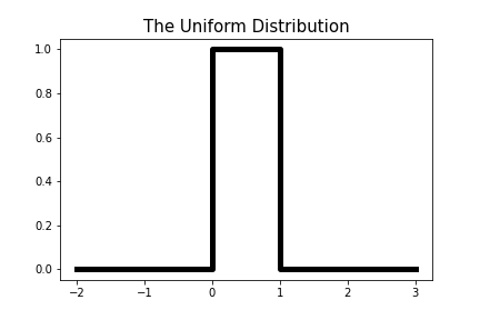
Figure 2-7. Graph of the probability density function of the uniform distribution over the interval [0,1].

The uniform distribution is extremely useful in computer simulations for generating random numbers from any other probability distribution. If you peek into the random number generators that Python uses, you would see the uniform distribution used somewhere in the underlying algorithms.

Distribution of Data: The Bell Shaped Normal (Gaussian) Distribution

A continuous probability ditribution better suited to model human height data (when restricted to one gender) is the bell shaped normal distribution, also called the Gaussian distribution. Samples from the normal distribution tend to congregate around an average value where the distribution peaks, called the mean $\mu$, then dwindle symmetrically as we get farther away from the mean. How far from the mean the distribution spreads out as it dwindles down is controlled by the second parameter of the normal distribution, called the standard deviation $\sigma$. About 68% of the data falls within one standard deviation of the mean, 95% of the data falls within two standard deviations of the mean, and about 99.7% of the data falls within three standard deviations of the mean.

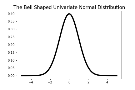
Figure 2-8. Graph of the probability density function of the bell shaped normal distribution with parameters $\mu =0$ and $\sigma =1$.

Values near the mean are more likely to be picked (or to occur, or to be observed) when we are sampling data from the normal distribution, and values near the minimum or maximum are less likely to be picked. This peaking near the mean value and decaying on the outer skirts of the distribution gives this distribution its famous bell shape. Note that there are other bell shaped continuous distributions out there, but the normal distribution is the most prevelant. It has a neat mathematical justification for this well deserved fame, based on an important theorem in probability theory called The Central Limit Theorem.

The Central Limit Theorem states that the average of many independent random variables, that all have the same distribution (not necessarily the normal distribution), is normally distributed. This explains why the normal distribution appears everywhere in society and nature. It models baby birth weights, student grade distributions, countries’ income distributions, distribution of blood pressure measurements, etc. There are special statistical tests that help us determine whether a real data set can be modeled using the normal distribution. We will expand on these ideas later in the probability chapter.

If you happen to find yourself in a situation where you are uncertain and have no prior knowledge about which distribution to use for your application, the normal distribution is usually a reasonable choice. In fact, among all choices of distributions with the same variance, the normal distribution is the choice with maximum uncertainty, so it does in fact encode the least amount of prior knowledge into your model.

The formula for the probability density function of the normal distribution for one random variable x (univariate) is:

and its graph for $\mu =0$ and $\sigma =1$ is plotted in Figure 2-8.

The formula for the probability density function for the normal distribution of two random variables x and y (bivariate) is:

and its graph is plotted in Figure 2-9.

The above bivariate formula can be written in more compact notation using the language of linear algebra:

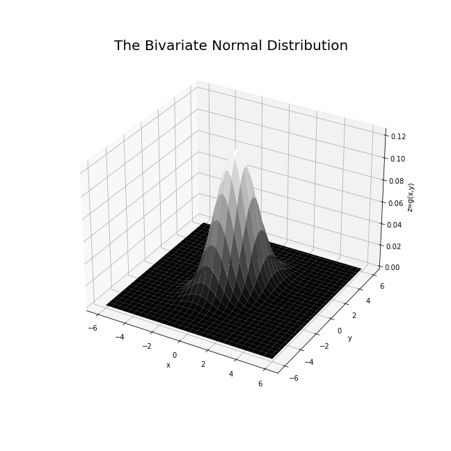
Figure 2-9. Graph of the probability density function of the bell shaped bivariate normal distribution.

In Figure 2-10, we sample 6000 points from the bivariate normal distribution.

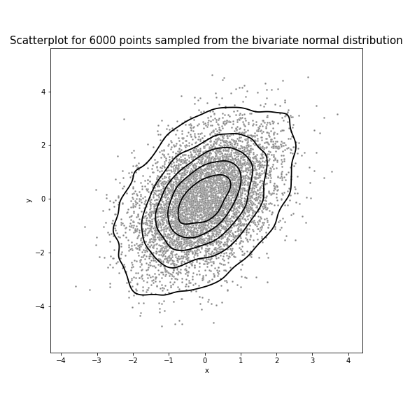
Figure 2-10. Sampling 6000 points from the bivariate normal distribution. Points near the center are more likey to be picked, and points away from the center are less likely to be picked.

Let’s pause and compare the formula of the probability density function for the bivariate normal distribution to formula of the probability density function for the univariate normal distribution:

• When there is only one random variable we only have one mean $\mu$ and one standard deviation $\sigma$.

• When there are two random variables, we have two means $\left(\begin{array}{c}{\mu }_1\\ {\mu }_2\end{array}\right)$, two standard deviations $\left(\begin{array}{c}{\sigma }_1\\ {\sigma }_2\end{array}\right)$. The product ${\sigma }^2$ will be replaced by the covariance matrix $\Sigma =\left(\begin{array}{cc}{\sigma }_1^2& \rho {\sigma }_1{\sigma }_2\\ \rho {\sigma }_1{\sigma }_2& {\sigma }_2^2\end{array}\right)$ and its determinant. $\rho$ is the correlation between the two random variables, which is the covariance of the two normalized versions of the random variables.

The same exact formula for the probability density function of the bivariate normal distribution generalizes to any dimension, where we have many random variables instead of only two random variables. For example, if we have 100 random variables, representing 100 features in a data set, the mean vector in the formula will have 100 entries in it, and the covariance matrix will have size $100\times 100$, with the variance of each random variable on the diagonal and the covariance of each of the 4950 pairs of random variables off the diagonal.

Distribution of Data: Other Important and Commonly Used Distributions

Almost everything you did not understand in this chapter will be revisited and mathematically formalized in Chapter 10 on Probability. Moreover, the same concepts will keep appearing in the upcoming chapters, so they will get reinforced as time evolves. Our goal for this chapter is to get exposed to the vocabulary of probability and statistics, and have a guiding map for the important ideas that frequently appear in AI applications. We also want to acquire a good probabilistic intuition for the following chapters without having to take a deep dive and delay our progress for no necessary reason.

There are many probability distributions out there. Each models a different type of real world scenario. The uniform and normal distributions are very common, but we have other important distributions that frequently appear in the AI field. Recall that our goal is to model the world around us in order to make good designs, predictions and/or decisions. Probability distributions help us make predictions when our models involve randomness or when we are uncertain about our outcomes.

When we study distributions, one frustrating part is that most of them have weird names that provide zero intuition about what kind of phenomena a given distribution would be useful for. This makes us either expend extra mental energy to memorize these names, or keep a distribution cheat sheet in our pocket. I prefer to keep a cheat sheet. Another frustrating part is that most text book examples involve either flipping a coin, rolling a die, or drawing colored balls from urns. This leaves us with no real life examples or motivation to understand the subject, as I never met anyone walking around flipping coins and counting heads or tails, except for The Joker in the Dark Night (a really good 2008 movie, where The Joker says some of my favorite and profound statements about randomness and chance, like this one, "The world is cruel. And the only morality in a cruel world is chance. Unbiased. Unprejudiced. Fair.”). I will try to amend this as much as I can in this book, pointing to as many real world examples as my page limit allows.

Some of the following distributions are mathematically related to each other, or follow naturally from others. We will explore these relationships in Chapter 10. For now, let’s name a popular distribution, state whether it is discrete (predicts a count of something that we care for) or continuous (predicts a quantity that exists in the continuum, such as the time needed to elapse before something happens: Careful, this is not the number of hours since the number of hours is discrete, but it is the length of the time period), state the parameters that control it, and its defining properties that are useful for our AI applications.

• The Binomial Distribution: This is discrete. It represents the probability of obtaining a certain number of successes when repeating one experiment, independently, multiple times. Its controlling parameters are n, the number of experiments we perform, and p, the predefined probability of success. Real world examples include predicting the number of patients that will develop side effects for a vaccine or a new medication in a clinial trial, predicting the number of ad clicks that will result in a purchase, or the number of customers that will default on their monthly credit card payments.

• The Poisson Distribution: This is discrete. It predicts the number of rare events that will occur in a given period of time. These events are independent or weakly dependent, meaning that the occurence of the event once does not affect the probability of its next occurence in the same time period. They also occur at a _ known and constant_ average rate $\lambda$. Thus, we know the average rate, and we want to predict how many of these events will happen during a certain time period. The Poisson distribution’s controlling parameter is the predefined rare event rate $\lambda$. Real world examples include predicting the number of babies born in a given hour, the number of people in a population who age past 98, the number of alpha-particles discharged from a radioactive system during a certain time period, the number of duplicate bills sent out by the IRS, the number of a not too popular product sold on a particular day, the number of typos that one page of this book contains, the number of defective items produced by a certain machine on a certain day, the number of people entering a store at a certain hour, the number of car crashes an insurance company needs to cover within a certain time period, and the number of earthquakes happening within a particular time period.

• The Geometric Distribution: This is discrete. It predicts the number of trials needed before we obtain a success, when performing independent trials each with a known probability p for success. The controlling parameter here is obviously the probability p for success. Real-world examples include estimating the number of weeks that a company can function without experiencing a network failure, the number of hours a machine can function before producing a defective item, or the number of people we need to interview before meeting someone who opposes a certain bill that we want to pass.

• The Exponential Distribution: This is continuous. It predicts the waiting time until an event occurs when it is known that the events occur at a constant rate $\lambda$. It is memoryless, in the sense that the remaining lifetime of an item which belongs to this exponential distribution is also exponential. The controlling parameter is the constant rate of event occurance $\lambda$. Real world examples include the amount of time we have to wait until an earthquake occurs, the amount of time before a terrorist attack strikes, the time until the default on a loan, or the time until a machine part fails. This is very useful for the reliability field, where the reliability of a certain machine part is calculated, hence statements such as 10-year guarantee, etc.

• The Weibull Distribution: This is continuous. It is widely used in engineering in the field of predicting products’ lifetimes. Again, 10 year guarantee statements are appropriate here as well. Here, a product consists of many parts, and if any of its parts fails, then the product stops working. For example, a car would not work if its battery fails, or if a fuse in its gearbox burns out. A Weibull distribution provides a good approximation for the lifetime of a car before it stops working, after accounting for its many parts and their weakest link (assuming we are not maintaining the car and resetting the clock). It is controlled by three parameters: the shape, scale, and location parameters. The exponential distribution is a special case of this distribution, because the exponential distribution has a constant rate of event occurance, but the Weibull distribution can model rates of occurence that increase or decrease with time.

• The Log-Normal Distribution: This is continuous. If we take the logarithms of each value provided in this distribution, then we get normally distributed data. Meaning in the beginning your data might not appear normally distributed, but try transforming it using the log function, then you would see normally distributed data. This is a good distribution to use when encounter skewed data with low mean value, large variance, and assumes only positive values. Just like the normal distribution appears when you average many independent samples of a random variable (using the central limit theorem), the log-normal distribution appears when you take the product of many positive sample values. Mathematically, this is due to an awesome property of log functions: The log of a product is a sum. This distribution is controlled by three parameters: shape, scale, and location parameters. Real world examples include the volume of gas in a petroleum reserve, and the ratio of the price of a security at the end of one day to its price at the end of the day before.

• The Chi-Squared Distribution: This is continuous. It is a distribution for the sum of squares of normally distributed independent random variables. You might wonder why would we care about squaring normally distributed random variables, then adding them up. The answer is that this is how we usually compute the variance of a random variable or of a data sample, and one of our main goals is controlling the variance, in order to lower our uncertainties. There are three types of significance tests associated with this distribution: The goodness of fit test, which measures how far off our expectation is from our observation, and the independence and homogeneity of features of data test.

• The Pareto Distribution: This is continuous. It is useful for many real world applications, such as, the time to complete a job assigned to a supercomputer (think machine learning computations), the household income level in a certain population, and the file size of the internet traffic. This distribution is controlled by only one parameter $\alpha$.

Let’s throw in few other distributions before moving on, without fussing about any of the details. These are all more or less related to the aforementioned distributions: The Student t-Distribution (continuous, similar to the normal distribution, but used when the sample size is small and the population variance is unknown), the Beta Distribution (continuous, produces random values in a given interval), the Cauchy Distribution (continuous, has to do with the tangents of randomly chosen angles), the Gamma Distribution (continuous, has to do with the waiting time until n events occur, instead of only one event, as in the exponential distribution), the Negative Binomial Distribution (discrete, has to do with the number of trials needed in order to obtain a certain number of successes), the Hypergeometric Distribution (discrete, similar to the binomial but the trials are not independent), and the Negative Hypergeometric Distribution (discrete, captures the number of dependent trials needed before we obtain a certain number of successes).

The Various Uses Of The Word Distribution

You might have already noticed that the word distribution refers to many different (but related) concepts, depending on the context. This inconsistent use of the same word could be a source of confusion and an immediate turn off for some people who are trying to enter the field.

Let’s list the different concepts that the word distribution refers to, so that we easily recognize its intended meaning in a given context:

• If you have real data, such as the Height Weight data in this chapter, and plot the histogram of one feature of your data set, such as the Height, then you get the emperical distribution of the height data. You usually do not know the underlying probability density function of the height of the entire population, also called distribution, since the real data you have is only a sample of that population, so you try to estimate it, or model it, using the probability distributions given by probability theory. For the height and weight features, when separated by gender, a Gaussian distribution is appropriate.

• If you have a discrete random variable, the word distribution could refer to either its probability mass function or its cummulative distribution function, which gives the probability that the random variable is less than or equal a certain value.

• If you have a continuous random variable, the word distribution could refer to either its probability density function or its cummulative distribution function, whose integral gives the probability that the random variable is less than or equal a certain value.

• If you have multiple random variables (discrete, continuous, or a mix of both), then the word distribution refers to their joint probability distribution.

A common goal is to establish an appropriate correpondence between an idealized mathematical function, such as a random variable with an appropriate distribution, and real observed data or phenomena, with an observed emperical distribution. When working with real data, each feature of the data set can be modeled using a random variable. So in a way a mathematical random variable with its corresponding distribution is an idealized version of our measured or observed feature.

Finally, distributions appear everywhere in AI applications. We will encounter them plenty of times in the next chapters, for example, the distribution of the weights at each layer of a neural network, and the distribution of the noise and the errors committed by various machine learning models.

Summary And Looking Ahead

In this chapter, we emphasized the fact that data is central to AI. We also clarified the differences between concepts that are usually a source of confusion: structured and unstructured data, linear and nonlinear models, real and simulated data, deterministic functions and random variables, discrete and continuous distributions, posterior probabilities and likelihood functions. We also provided a map for the probability and statistics needed for AI without diving into any of the details, and we introduced the most popular probability distributions.

If you find yourself lost in some new probability concept, you might want to consult the map provided in this chapter and see how that concept fits within the big picture of probability theory, and most importantly, how it relates to AI. Without knowing how a particular mathematical concept relates to AI, you are left with having some tool that you know how to turn on, but you have no idea what it is used for.

We have not yet mentioned random matrices and high dimensional probability. In these fields, probability theory, with its constant tracking of distributions, expectations and variances of any relevant random quantities, merges with linear algebra, with its hyperfocus on eigenvalues and various matrix decompositions. These fields are very important for the extremely high dimensional data that is involved in AI applications, and they will have their own Chapter 12 in this book.

In the next chapter, we learn how to fit our data into a function, then use this function to make predictions and/or decisions. Mathematically, we find the weights (the $\omega$’s) that characterize the strengths of various interactions between the features of our data. When we characterize the involved types of interactions (the formula of the fitting function, called the learning or training function) and the strengths of these interactions (the values of the $\omega$’s), we can make our predictions. In AI, this one concept of characterizing the fitting function with its suitable weight values can be used successfully for computer vision, natural language processing, predictive analytics (like house prices, time until maintainance etc.), and many other applications.