Chapter 2. Design a tabular BI semantic model

The skills necessary to develop a tabular model for SQL Server Analysis Services (SSAS) are much different than the skills required to develop a multidimensional model. In some ways, the tabular modeling process is much simpler and more flexible than the multidimensional modeling process. Although it is not required to transform the source data for a tabular model into a star schema, the development steps are in general easier if you work from a star schema and the processing necessary to load a tabular model with data can often run faster. For this reason, in this chapter we use the same data source introduced in the previous chapter to walk through key development and administrative tasks for a tabular model. In addition, we explore your options for keeping the data in your tabular model up-to-date, either by importing the data into the model on a periodic basis or by configuring the model for real-time data access.

Skills in this chapter:

Design and publish a tabular data model

Configure, manage, and secure a tabular model

Develop a tabular model to access data in near real time

1. Open Microsoft SQL Server Data Tools for Visual Studio 2015 (SSDT). If you have trouble connecting to the tabular instance in a later step, you should right-click SSDT in the Start Menu or in the All Apps list, and then click Run As Administrator to elevate permissions while developing the tabular model.

2. In the File menu, point to New, and then click Project.

3. In the New Project dialog box, click Analysis Services in the Business Intelligence group of templates, and then click Analysis Services Tabular Project. At the bottom of the dialog box, type a name for the project, select a location, and optionally type a new name for the project’s solution. The project for the examples in this chapter is named 70-768-Ch2.

4. When you create a new tabular project, the Tabular Model Designer dialog box prompts you for the workspace server name and compatibility level. If necessary, type the SSAS tabular server name (or server and instance name, such as localhostTABULAR). Performance during model development is generally better if you work with a local tabular server. Keep the default compatibility level, SQL Server 2016 RTM (1200) to enable features specific to the SQL Server 2016 version of SSAS tabular on which the exam tests your knowledge. The other compatibility levels are included for backward compatibility. Click OK to create the project and add the Model.bim file to your project in the Solution Explorer window.

When you add the Model.bim file to your project, SSDT creates a workspace database on the SSAS server. Each model has its own workspace database that you can recognize in SSMS by its name that is a concatenation of the database name specified in the project’s properties (described in the “Select a deployment option, including Processing Option, Transactional Deployment, and Query Mode” section of this chapter) and a globally unique identifier (GUID). You should not use SSMS to make changes to the workspace database while the model is open in SSDT to avoid damaging the model.

Your next step is to add data to your project. Whereas a multidimensional database requires your data to be in a relational data source, a tabular database can import data from the following data sources:

Microsoft SQL Server 2008 and later

Microsoft Azure SQL Database

Microsoft Azure SQL Data Warehouse

Microsoft Analytics Platform System

Microsoft Access 2010 and later

Oracle 9i and later

Teradata V2R6 and later

Sybase 15.0.2

Informix

IBM DB2 8.1

OLE DB or ODBC

Microsoft SQL Server 2008 and later Analysis Services

Microsoft Reporting Services

Microsoft Azure Marketplace

Data feed in Atom 1.0 format or exposed as Windows Communication Foundation (WCF) Data Service

Microsoft Excel 2010 and later

Text file

Office Database Connection (.odc) file

Let’s add a few tables from the WideWorldImportersDW database to the tabular model. To do this, perform the following steps:

1. Click Import From Data Source on the Model menu, click Microsoft SQL Server on the Connect To A Data Source page of the Table Import Wizard, and click Next.

2. On the Connect To A Microsoft SQL Server Database page of the wizard, type the name of your SQL Server in the Server Name box, set the authentication if not using Windows authentication, select WideWorldImportersDW in the Database Name drop-down list, and click Next.

3. On the Impersonation Information page of the wizard, you can choose one of the following options:

Specific Windows User Name And Password Use this option when you need to connect to your data source with a specific login, such as a Windows login with low privileges that has read permission to the data source. This information is kept in memory only and not persisted on disk. If the model is not in memory when you attempt to deploy it from SSDT, you are prompted to provide the credentials.

Service Account Use this option to connect to the data source by using the account running the SSAS service. If you use this option, be sure that it has read permission on the database.

Unattended Account Ignore this option because it is not supported.

4. Click Next to continue to the Choose How To Import The Data page of the wizard. This page displays only when you are connecting to a relational data source. Here you can choose one of the following options:

Select From A List Of Tables And Views To Choose The Data To Import Use this option to choose one or more tables or views from the data source.

Write A Query That Will Specify The Data To Import Use this option when you want to create a single table in the model based on a Structured Query Language (SQL) query. Your query can be as simple or complex as you need to return the required results from the data source. However, you cannot call a stored procedure by using this option.

To follow the examples in this chapter, click the Select From A List Of Tables And Views To Choose The Data To Import option, and click Next to see the list of available tables and views.

5. Select the check box to the left of each of the following tables: City, Customer, Date, Employee, Stock Item, and Sale.

6. You can apply a filter to an individual table to eliminate specific columns or remove rows based on criteria that you supply. For example, let’s remove the Sale Key and Lineage Key columns from the Sale table. Select the Sale table in the list of tables and views, and then click Preview And Filter button. A dialog box displays a preview of the rows in the table. Here you can clear the check box for the Sale Key column, as shown in Figure 2-1.

7. You can apply a row filter by clicking the arrow in the column header to open the AutoFilter menu, the contents of which depend on the data type of the column. Figure 2-2 shows the AutoFilter menu for a date column. You can point to Date Filters to display a list of filtering options, such as Before, After, and Last Year, among others. If the column is numeric, the filtering options include Equals, Greater Than, and Between, to name a few. Text filtering options include Begins With, Contains, and several others. As an alternative approach, you can individually clear or select check boxes in the list of items that display in the Autofilter menu. However, it’s possible that the item list is not complete, as indicated by the Not All Items Showing message. Click OK to close the Autofilter menu, and then click OK to close the Preview Selected Table dialog box.

8. After adding and optionally filtering the tables you need for the models, click Finish on the Select Tables And Views page of the Table Import Wizard. SSDT then executes the queries against your relational data source and copies the data into memory on the SSAS server. This version of the model is not deployed yet, but exists on the server nonetheless as a result of creating the project as described at the beginning of this section. Tabular models on the SSAS server are managed by the tabular engine, also known as the xVelocity engine.

9. Click Close to close the Table Import Wizard after the data is successfully copied. After the tables are loaded, the model designer displays in SSDT with one tab per table, as shown in Figure 2-3. Notice the status bar at the bottom of the page in which you can see the number of rows imported for the current table.

You can continue to load data from other data sources by repeating this process. There is no requirement for all data to be combined into a single source before you load it into the tabular model or that all data comes from a single type of data source, such as a relational database. Your primary consideration should be whether the data from different sources are related, and how much transformation of the data is necessary for it to be useful in the model. If you need to perform complex or many transformations, you should consider using an extract-transform-load (ETL) tool to prepare the data in advance of loading it into a tabular model, or even consider building a data mart or data warehouse to transform and conform the data as needed.

Let’s add a simple measure to the Sale table to compute the total sales by summing the Total Excluding Tax column. To do this, perform the following steps:

1. Click the Sale tab, and then click a cell in the measure grid. The measure grid is the section of the model designer that displays below the data grid. You can click any cell, but a good habit to develop is to place measures in the cells in the first few columns of the grid to make it easier to find them later if you need to make changes.

2. After you click a cell in the measure grid, use the formula bar above the data grid to type a measure name followed by a colon, an equal sign, and a DAX expression (shown in Listing 2-1), as shown in Figure 2-4. In this measure expression, the SUM aggregate function is applied to the [Total Excluding Tax] column in the Sale table. After you press Enter, SSDT computes the result and displays it next to the measure name in the calculation grid below the data grid in the model designer.

LISTING 2-1 Total Sales measure expression

Click here to view code image

---

Total Sales := SUM(Sale[Total Excluding Tax])

---

The formula bar in the model designer has several features that help you write and review DAX formulas easier:

Syntax coloring You can identify formula elements by the color of the font: functions display in a blue font, variables in a cyan font, and string constants in a red font. All other elements display in a black font.

IntelliSense IntelliSense helps you find functions, tables, or columns by displaying potential matches after you type a few characters. In addition, it displays a wavy red underscore below an error in your expression.

Formatting You can improve legibility of complex or long expressions by pressing ALT+Enter to break the expression into multiple lines. You can also type // as a prefix to a comment.

Formula fixup As long as your tabular model is set to compatibility level 1200, the model designer automatically updates all expressions that reference a renamed column or table.

Incomplete formula preservation If you cannot resolve an error in an expression, you can save and close the model, if it is set to compatibility level 1200, and then return to your work at a later time.

Next, create additional measures in the specified tables as shown in Table 2-1. Unlike a multidimensional model in which you create measures only as part of a measure group associated with a fact table, you can add a measure to any table in a tabular model.

Each measure has the following set of editable properties that control the appearance and behavior of the measure in client applications:

Display Folder You can type a name to use as a container for one or more measures when you want to provide a logical grouping for several measures and thereby help users more easily locate measures within a list of many measures. The use of this feature depends on the client application. Excel includes the Display Folder in the PivotTable Field List, but the Power View Field List does not.

Description You can type a description to provide users with additional information about a measure. This feature requires the client application to support the display of a description. Excel does not display the measure’s description, but Power View includes the description in a tooltip when you hover the cursor over the measure in the Power View Field List.

Format You can apply an appropriate format to your measure by choosing one of the following values in the Format drop-down list: General, Decimal Number, Whole Number, Percentage, Scientific, Currency, Date, TRUE/FALSE, or Custom. If the selected format supports decimal places, the Decimal Places property is added to the Properties window, which you can configure to define the measure’s precision. Some format types allow you to specify whether to show thousand separators. If you select the Currency format, you can also configure the Currency Symbol property. Selection of the Custom format adds the Format String property, which you can configure to use a Visual Basic format string.

Measure Name If you need to rename the measure, you can type a new name for this property. A measure name must be unique within your tabular model and cannot duplicate the name of any column in any table. Consider assigning user-friendly names that are meaningful to users and use embedded spaces, capitalization, and business terms.

Table Detail Position This property defines behavior for specific client tools, such as Power View in SharePoint. When you set this property, a user can double-click the table to add a default set of fields to a table.

Let’s set the format for each of the measures, as shown in Table 2-2.

Because the WideWorldImportersDW database tables have foreign key relationships defined in the Sale table, the addition of the dimension tables associated with that fact table also adds corresponding relationships in the model. Click the Diagram icon in the bottom right corner of the model designer (or point to Model View in the Model menu, and then select Diagram View) to see a diagram of the model’s tables and relationships, as shown in Figure 2-5.

You can review the Properties window to understand an individual relationship by clicking its line in the diagram. For example, if you click the line between Employee and Sale, you can review the following three properties:

Active Most of the time, this value is set to True and the relationship line is solid. When this value is set to False, the relationship line is dashed. This property is the only one that you can change in the Properties window.

Foreign Key Column This column contains the foreign key value that must be resolved by performing a lookup to the primary key column. For the relationship between Employee and Sale, the foreign key column is set to Sale[Salesperson Key].

Primary Key Column This column contains the primary key column holding unique values for a lookup. For the relationship between Employee and Sale, the primary key column is set to Employee[Employee Key].

A relationship is not always automatically created when you add tables. As one example, if your tables come from a relational data source and no foreign key relationship exists between tables, you must define the relationship manually. As another example, if you add the tables in separate steps, the relationship is not inherited by the tabular model. Last, if your tables come from different data sources, such as when one table comes from a Microsoft Excel workbook and another table comes from a text file, there is no predefined relationship to inherit and therefore you must add any needed relationships.

To manually add a relationship, you can use one of the following techniques:

Drag and drop (Diagram View) In the Diagram view, you can drag the foreign key column from one table and drop it on the corresponding primary key column in another table to create a relationship.

Column relationship (Grid View) To access the Grid view, click the tab for the table that has the foreign key column, right-click the foreign key column, and click Create Relationship. In the Table 2 drop-down list, select the table containing the primary key column, and then click the primary key column in the list that displays. You can then specify the cardinality and filter direction as described later in this section.

Manage Relationships dialog box On the Table menu, select Manage Relationships to open the Manage Relationships dialog box, as shown in Figure 2-6. In this dialog box, you have a comprehensive view of all relationships defined in the tabular model. The dialog box includes buttons to create a new relationship, edit an existing relationship, or delete a relationship.

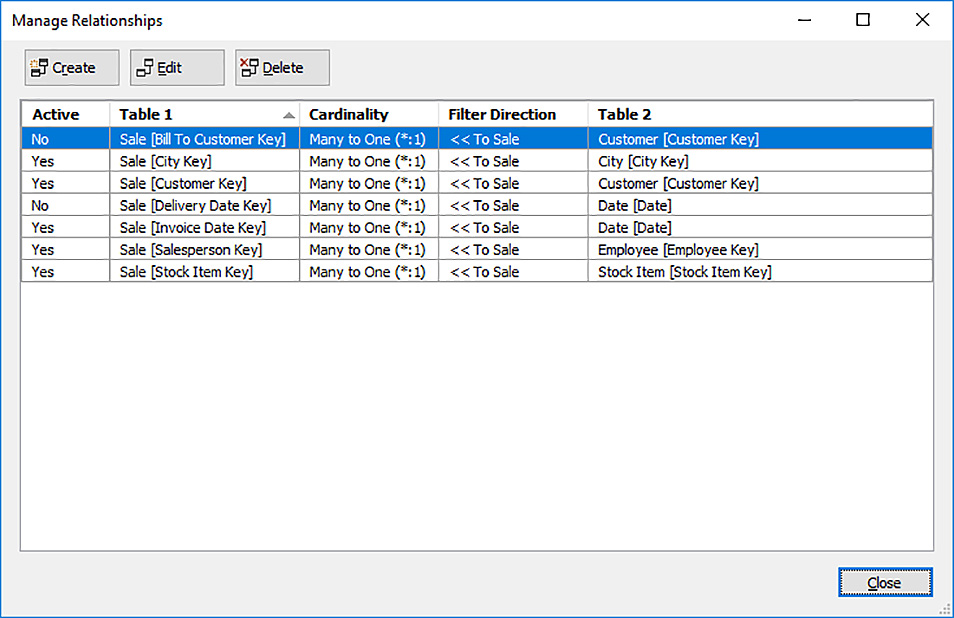
In the Manage Relationships dialog box, you can tell at a glance the cardinality of each relationship and the filter direction. These settings directly influence the behavior of queries that involve these tables.

Many To One Many-to-one cardinality describes a relationship in which Table 1 can have many rows that reference a single row in Table 2. For example, the Sale table can have many rows that refer to a single stock item, or a single customer.

One To One One-to-one cardinality describes a relationship in which only one row in Table 1 refers to a single row in Table 2. None of the tables in the tabular model have one-to-one cardinality.

Regardless of the cardinality type that you define for a relationship, the lookup column in Table 2 must contain unique values in each row. Although a null or blank value is valid, you cannot have multiple rows that are null or blank in the lookup column.

Furthermore, the lookup column must be a single column. You cannot use composite keys in a table. You must combine multiple columns into a single column prior to loading the data into your model, or by creating a calculated column. (Calculated columns are described later in this section.)

Let’s look at an example of each type of filter direction to understand the ramifications of each option by performing the following steps:

1. First, consider the relationship between the Sale and City table for which the filter direction is set To Sale, a one-directional filter. On the Model menu, click Analyze In Excel, and click OK in the Analyze In Excel dialog box to open a new Excel workbook connected to your model.

2. In the PivotTable Fields list, select the following check boxes: Sale Count, City Count, and Sales Territory (in the City table).

In the resulting PivotTable, shown in Figure 2-7, the row labels are values in the Sales Territory column from the City table. Because of the one-directional filter between Sale and City, SSAS uses each sales territory to filter the Sale table and compute the Sales Count value. In other words, SSAS starts by filtering the Sale table to include only rows for cities that have the value External in the Sales Territory column and counts the rows remaining in the filtered Sale table. Then it repeats the process to filter the Sale table for the Far West sales territory and counts the rows in the Sale table, and so on. Each measure value in the Sales Count column is the result of a separate filter based on a value in the City table applied to the Sale table. The City Count value counts rows in the City table, and uses the Sales Territory filter from the same table and computes correctly.

3. Now let’s add another row label to the PivotTable to summarize the results by both Sales Territory and Calendar Year. In the PivotTable Fields List, expand the More Fields folder for the Date table, and drag Calendar Year below the Sales Territory field in the Rows pane to produce the PivotTable for which a few rows are shown in Figure 2-8.

Now the Sale Count values are computed correctly because the Sale table is filtered by Sales Territory on rows 2 and 8, and by both Sales Territory and Calendar Year on rows 3 through 7, and rows 9 through 13 because both the City and Date tables have a one-directional filter for the Sale table. However, values in the City Count column compute correctly only on rows 2 and 8 because they are filtered by Sales Territory, which is in the same table as the City Count column. For the other rows, SSAS is unable to apply an additional filter by Calendar Year because the Date table has no relationship with the City table, nor should it. Consequently, the City Count for a specific sales territory repeats across all years for that sales territory.

4. To change this behavior, you can set up a bidirectional relationship between City and Sale by leaving Excel open, switching back to SSDT, and clicking Manage Relationships on the Table menu.

5. In the Manage Relationships dialog box, select the row with Sale [City Key] in the Table 1 column, and City [City Key] in the Table 2 column, and click Edit.

6. In the Filter Direction drop-down list, select To Both Tables. Click OK to close the Edit Relationship dialog box, and then click Close to close the Manage Relationships dialog box. Press CTRL+S to save the model.

7. Switch back to Excel and click Refresh in the Analyze tab of the ribbon to update the PivotTable, shown in Figure 2-9. Now the City Count values change for each year. For each row containing a Calendar Year, SSAS filters the Sale table by sales territory and by calendar year, and then filters the City table by using the City Key values in the filtered Sale Table. To compute City Count, it counts the rows in the filtered City table.

The ability to use a bidirectional filter in a relationship means you can now model a many-to-many relationship in a tabular model rather than create complex DAX expressions, which was the only way to handle a many-to-many scenario in previous versions of SSAS. You can simulate a many-to-many relationship in the tabular model like the one described in Chapter 1 by adding a new table to the model based on a query. To do this, perform the following steps:

1. Switch back to SSDT, and then, on the Model menu, click Import From Data Source, click Next in the wizard, type the server name for your SQL Server, and select WideWorldImportersDW in the Database Name drop-down list.

2. Click Next, select the Service Account option for impersonation, click Next, select the Write A Query That Will Specify The Data To Import option, click Next, and then type the query shown in Listing 2-2.

LISTING 2-2 Query statement to create Sales Reason dimension

Click here to view code image

---

SELECT
    1 AS SalesReasonKey, 'Value' AS SalesReason
UNION
SELECT
    2 AS SalesReasonKey, 'Manufacturer' AS SalesReason
UNION
SELECT
    3 AS SalesReasonKey, 'Sales Person' AS SalesReason;

---

3. Click Finish, and then click Close. In the model designer, right-click the tab labeled Query, click Rename, and type Sales Reason.

4. Next, repeat these steps to add the bridge table by using the query shown in Listing 2-3.

LISTING 2-3 Named query statement to create Sales Reason Bridge

Click here to view code image

---

SELECT
    CAST(1 AS bigint) AS [Sale Key],
    1 AS SalesReasonKey
UNION
SELECT
    CAST(1 AS bigint) AS [Sale Key],
    2 AS SalesReasonKey
UNION
SELECT
    CAST(1 AS bigint) AS [Sale Key],
    3 AS SalesReasonKey
UNION
SELECT
    CAST(2 AS bigint) AS [Sale Key],
    1 AS SalesReasonKey;

---

5. Rename the query as Sales Reason Bridge. You can do this by replacing the Friendly Name when you add the query to the Table Import Wizard, or after the table is added to the model. Because this table is used only for modeling purposes, you can hide it by right-clicking its tab, and clicking Hide From Client Tools, just as you can hide a column.

6. Now you need to define relationships between Sale and Sales Reason Bridge. Switch to the Sale table, right-click the Sale Key column header, and click Create Relationship. In the Create Relationship dialog box, select Sales Reason Bridge in the Table 2 drop-down list table, and select To Both Tables in the Filter Direction drop-down list. Notice the One To Many relationship between the tables is automatically set for you. Click OK.

7. You also need a relationship between Sales Reason Bridge and Sales Reason. Switch to the Sales Reason Bridge table, right-click the Sales Reason Key column header, and click Create Relationship. In the Table 2 drop-down list, select Sales Reason. Keep the cardinality and filter direction settings, and click OK. Click CTRL+S to save the model.

8. You can check the results of modeling this many-to-many relationship by creating a PivotTable to show sales counts by sales reason. Click Analyze In Excel in the Model menu, click OK, and then set up the PivotTable by selecting the Total Sales, Sales Count, WWI Invoice ID (from the Sale table) and SalesReason (from the Sales Reason table) check boxes. Partial results are shown in Figure 2-10. No direct relationship exists between Sales Reason and Sale, but the subtotal for each invoice reflects the correct count of sales, which does not match the sum of the individual rows.

When you create a new relationship between two tables, the filter direction is one-directional by default. However, you can change this behavior for the current model by clicking the Model.bim file in Solution Explorer, and then, in the Properties window, choosing Both Directions in the Default Filter Direction drop-down list. If you want to change the default for all new tabular projects, click Options on the Tools menu, expand Analysis Services Tabular Designers in the navigation pane on the left, click New Project Settings, and then select Both Directions in the Default Filter Direction drop-down list.

To create a hierarchy in a tabular model, perform the following steps:

1. Switch to the Diagram view in SSDT.

2. Let’s create a hierarchy in the Date dimension to support drill down from year to month to date. To do this, right-click Calendar Year Label, click Create Hierarchy, and type Calendar as the new hierarchy name. You can then either drag the next column, Calendar Month Label, below Calendar Year Label in the hierarchy, or right-click the column, point to Add To Hierarchy, and then click Calendar.

3. Repeat this step to add Date to the hierarchy. You can see the resulting hierarchy and its columns in the Diagram view, as shown in Figure 2-11.

4. You can now test the hierarchy. If Excel remains open from a previous step, you can click Refresh on the PowerPivot Tools Analyze tab of the ribbon. Otherwise, click Analyze In Excel on the Model menu, and click OK in the Analyze In Excel dialog box. In Excel, select the following check boxes in the PivotTable Fields List: Total Sales and Calendar.

5. In the PivotTable, you can expand CY2013 and CY2013-Apr to view each level of the hierarchy related to April 2013, as shown in Figure 2-12.

The behavior of the hierarchy is normal, but its sort order is not because the default sort order of values in a column with a Text data type is alphabetical. However, the sort order for months should be chronological by month number. In a tabular model, you can fix this by configuring a Sort By Column to manage the sort order. If you have control over the design over the data source, you can add a column to define a sort order for another column. Otherwise, you need to modify the table structure in your model, as described in the “Calculated columns” section later in this chapter.

6. To fix the sort order for Calendar Month Label, switch back to SSDT from Excel, toggle to the Grid view, and select the Date tab at the bottom of the model designer.

7. Select the Calendar Month Label column to view its properties in the Properties window.

8. In the Sort By Column property’s drop-down list, select Calendar Month Number.

9. Press CTRL+S to save the model, and then switch back to Excel. In the Analyze tab of the ribbon, click Refresh. The months for CY2013 now sort in the correct sequence from CY2013-Jan to CY2013-Dec.

Another scenario for which you can consider partitioning is a rolling window strategy. In this case, your business requirements can be to support analysis of sales over the last 24 months. If you partition by month, you can add a new partition as sales data comes in for a new month and remove the oldest partition so that you always have 24 partitions at a time. The addition of a new partition and removal of an existing partition is much faster than reloading the entire 24 months of data into the tabular model.

By default, each table in your tabular model is contained in one partition. You can define more partitions in the Partition Manager, which you open by selecting Partitions on the Table menu. Figure 2-13 shows the Partition Manager for the Sale table. Here you can see the name and last processed date of the single partition that currently exists in the tabular model as well as a preview of the rows in the selected partition.

You use the Partition Manager to manually define a specific number of partitions. If each partition is based on the same source, you define a filter for each partition. As an example, let’s say that data for each Bill To Customer comes into the source system at different times and you want to refresh the tabular model for each Bill To Customer separately. To change the filter for the existing partition, perform the following steps:

1. Click the drop-down arrow in the Bill To Customer Key column, clear the (Select All) check box, select the 0 check box, and click OK.

2. Change the partition name by typing Bill To Customer 0 after the existing name, Sale, in the Partition Name text box.

3. Next, click Copy to create another partition and then change the filter for the new partition to the Bill To Customer key value of 1, and change its name to Sale Bill To Customer 1.

4. Create a final partition by copying either partition, setting the Bill To Customer key to 202, and changing its name to Bill To Customer 202.

5. Click OK to save your changes, and then, on the Model menu, point to Process, and then select Process Table to replace the single partition for Sale in your tabular model with the three new partitions.

When your partitioning strategy is more dynamic, usually because it is based on dates, you can use a script to define partitions instead of Partition Manager. You can then create a SQL Server Integration Services (SSIS) package to execute the script by using an Analysis Services DDL Task, and then schedule the SSIS package to run on a periodic basis.

To generate a script template, perform the following steps:

1. Right-click the project in Solution Explorer, and select Deploy. SSDT deploys your project to the server you identified when you created the project using the name of your project as the database name, but you can change these settings in the project’s properties.

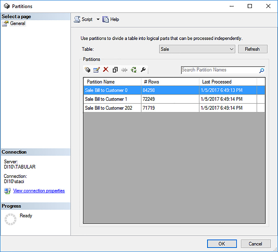
2. Next, open SQL Server Management Studio (SSMS), connect to the tabular instance of Analysis Services, expand the Databases folder, expand the 70-768-Ch2 database, expand the Tables folder, right-click the Sale table, and select Partitions to open the Partitions dialog box, as shown in Figure 2-14.

3. Click the Script drop-down arrow, select Script Action To New Query Window, and click Cancel to close the Partitions dialog box. You can then update the script that displays in the query window by replacing the sections of the script with a new name for the partition and a revised query, as shown by the bold text in Listing 2-4. Although this listing does not include the annotations, you can keep the annotations in the script if you like.

LISTING 2-4 Create a new partition

Click here to view code image

---

{
  "createOrReplace": {
    "object": {
      "database": "70-768-Ch2",
      "table": "Sale",
      "partition": "Sale Bill To Customer 100"
    },
    "partition": {
      "name": "Sale Bill To Customer 100",
      "source": {
        "query": "SELECT [Fact].[Sale].* FROM [Fact].[Sale]
                  WHERE ([Bill To Customer Key] = 100)",
        "dataSource": "SqlServer localhost WideWorldImportersDW"
      }
    }
  }
}

---

4. Be sure to select 70-768-Ch2 in the Available Databases drop-down list, and then click Execute, or press F5 to execute the script.

5. Right-click the Sale table in the Object Explorer window, and select Process Table.

6. In the Process Table(s) dialog box, click OK to perform a Process Default operation on the Sale table. (We explain processing operations in more detail in Skill 2.2.)

7. Click Close in the Data Processing dialog box when processing is complete.

8. Check to confirm the addition of the new partition by right-clicking the Sale table in the Object Explorer window, and selecting Partitions to open the Partitions dialog box. Because there is no Bill To Customer key value of 100 in the table, the new partition appears in the dialog box with a last processed date but zero rows.

To create a new perspective, perform the following steps:

1. Point to Perspectives on the Model menu, and select Create And Manage.

2. In the Perspectives dialog box, click New Perspective, and type a name for the perspective, such as Stock Items By Date.

3. Scroll down, expand Date, and select the check box for each of the following fields: Calendar Month Label, Calendar Year Label, Date, and Calendar.

4. Expand Sale, and select the check box for Sales Count and Total Sales.

5. Next, expand Stock Item, and select the check box for the following fields: Brand, Color, Size, and Stock Item.

6. Click OK to save the perspective.

7. You can test the perspective by selecting Analyze In Excel on the Model menu, and then, in the Analyze In Excel dialog box, select Stock Items By Date in the Perspective drop-down list. Click OK to open Excel. The PivotTable Fields list now shows a subset of the available fields as defined by the perspective, as shown in Figure 2-15. Close the workbook when your review is finished.

When a user connects to a tabular model directly from Excel, the Data Connection Wizard displays the option to connect to the tabular model (called a Cube in the user interface) or to the perspective. In other client applications, you must specify replace the model name with the perspective name in the Cube property of the connection string.

A table contains columns for FirstName and LastName, but you need to display a single column with the values concatenated like “LastName, FirstName.”

A table contains null values and you want to display a default value, such as “NA.”

You need to perform a mathematical operation on values in two separate columns to derive a new scalar value.

You need unique values in a column to use as a lookup.

To resolve any of these situations, you can create a calculated column to define a new column in the table and populate it by using a DAX expression. There is no limitation on the data type that you assign to a calculated column, nor is there any limitation on the number of calculated columns that you can add to a table. That said, bear in mind that the data in a calculated column is stored in memory just like data imported from a data source, unlike a measure which is computed at query time.

In general, to add a calculated column, click the cell in the first row of the column labeled Add Column, and then type the expression for the calculated column in the formula bar. You do not provide a name for the calculated column in the expression as you do for a measure. Instead, after adding the expression, select the column, and then type the name in the Column Name property in the Properties window.

Enhance the 70-768-Ch2 model in SSDT by adding the calculated columns shown in Table 2-3. Refer to Chapter 3 to review these types of DAX expressions.

At this point, the tabular model is ready to explore using any tool that is compatible with SSAS, such as Excel or SSRS, but it is not yet set up as well as it can be. There are more dimensions and fact tables to add as well as many configuration changes to the dimension and cube to consider and implement that you explore in Skills 1.2 and 1.3.

A new feature in SQL Server 2016 Analysis Services, which requires your model to be set to a compatibility level of 1200, is the ability to create a calculated table. A calculated table is built solely by using a DAX expression. You can select a few columns from another table in the model, combine columns from separate tables, or transform and filter data to restructure it as a separate table. Use this feature sparingly because the addition of a calculated table to your model requires more memory on the SSAS server to store its data and increases the model’s processing time.

One use case for the addition of a date table is to support a roleplaying Date dimension. In the Sale table, there are two date columns—Invoice Date Key and Delivery Date Key. Rather than use DAX to change a query’s context from Invoice Date to Delivery Date, you can set up a calculated table for Delivery Date, and then define a relationship between the new date table and the Delivery Date Key column in the Sale table.

To create the date table, perform the following steps:

1. Click New Calculated Table on the Table menu, or click the Create A New Table Calculated From A DAX Formula tab at the bottom of the model designer.

2. In the formula bar above the new empty table grid, type a DAX expression or query that returns a table. For example, you can use a simple expression, such as =’Date’ to copy an existing roleplaying dimension table, Date.

A simpler method to create a date table is to use one of the following DAX functions:

CALENDAR Use this function to create a table with a single date column. You define the date range by providing a start and end date.

CALENDARAUTO Use this function to create a table with a single date column. The date range is determined by the model designer, which uses the earliest and latest dates found in any column in any table in the model.

Regardless of the method you use, you can then work with the table just like any other table for which data was imported in to the model. That means you can rename it, define relationships, add calculated columns, and configure properties.

Before deployment, SSAS stored your model in memory as a workspace database, which you can also access in SSMS. This workspace database stores the data that you added to the model by using the Table Import Wizard. When you view data in the model designer, or use the Analyze In Excel feature, SSAS retrieves the data from the workspace database. There are properties associated with the model that manage the behavior of the workspace database. Click the Model.bim file in Solution Explorer to view the following properties in the Properties window:

Data Backup You can change the setting from the default, Do Not Backup To Disk, to Backup To Disk to create a backup of the workspace database as an ABF file each time you save the Model.bim file. However, you cannot use the Back To Disk option if you are using a remote SSAS instance to host the workspace database.

Workspace Database This property cannot be changed. It displays the name that SSAS assigns to the workspace database.

Workspace Retention This setting determines whether SSAS keeps the workspace database in memory when you close the project in SSDT. The default option, Unload From Memory, keeps the database on disk, but removes it from memory. SSDT loads the model faster when you next open the project when you can choose the Keep In Memory option. The third option, Delete Workspace, deletes the workspace database from both memory and disk, which takes the longest time to reload because SSAS requires additional time to import data into the new workspace database. You can change the default for this setting if you open the Tools menu, select Options, and open the Data Modeling page in the Analysis Server settings.

Workspace Server This property specifies the server you use to host the workspace database. For best performance, you should use a local instance of SSAS.

1. Right-click the project name in Solution Explorer and select Properties.

2. In the 70-768-Ch2 Property Pages dialog box, select the Deployment page, as shown in Figure 2-16, and then update the Server text box with the name of your SSAS server if you need to deploy to a remote server rather than locally.

The following additional deployment options are also available on this page:

Processing Option Just as you can with multidimensional databases, you can specify whether to process the tabular model after deployment, and what type of processing to perform. When this option is set to Default, which is the default setting, SSAS processes only the objects that are not currently in a processed state. You can change this setting to Do Not Process if you want to perform processing later, or to Full if you want the database to process all objects whenever you deploy your project from SSDT. In Skill 2.2, “Configure, manage, and secure a tabular model,” we explain these and other processing options in greater detail.

Transactional Deployment When the value in this option is False, the deployment does not participate in a transaction with processing. Consequently, if processing fails, the model is deployed to the server, but remains in an unprocessed state. If you change this option’s value to True, deployment rolls back if processing fails.

3. When you are ready to create the database on the server, right-click the project in Solution Explorer, and click Deploy.

The first time you perform this step, the deployment process creates the database on the server and adds any objects that you have defined in the project. Each subsequent time that you deploy the project, as long as you have kept the default deployment options in the project properties, the deployment process preserves the existing database and adds any new database objects, and updates any database objects that you have modified in the project.

4. You can check the tabular model on the server by opening SSMS and connecting to the tabular instance of Analysis Services. In Object Explorer, expand the Databases folder, expand the 70-768-Ch2 folder, and then expand the Connection and Tables folders to review the objects in each folder, as shown in Figure 2-17.

If your tabular model is set to a lower compatibility level (1100 or 1103), you have the following two additional options available in the project’s properties:

Query Mode You use this option to determine the type of storage that SSAS uses for the tabular model. You can choose one of the following options:

DirectQuery This mode stores metadata on the SSAS server and keeps the data in the relational storage as described in Skill 2.3.

DirectQuery With In-Memory This option is a hybrid mode. SSAS resolves queries by using DirectQuery by default. It retrieves data from cache only if the client connection string requests a change in mode as described in Skill 2.3.

In-Memory This mode stores both metadata and data imported from data sources on the SSAS server.

In-Memory With DirectQuery This is another type of hybrid mode. With this option, queries are resolved from the data stored in cache on the SSAS server unless the client connection string switches the query to DirectQuery mode as described in Skill 2.3.

Impersonation Settings This option is applicable only if you set the Query Mode option to DirectQuery. If you keep the default value of Default, user connections to the tabular model use the credentials set in the Table Import Wizard to connect to the backend database. You can change this to ImpersonateCurrentUser if you want SSAS to pass the user’s credentials to the backend database.

You can also change data source impersonation after deploying the model to the server. In SSMS, connect to the Analysis Services server, and then, in Object Explorer, expand the Databases folder, the folder for your database, and the Connections folder. Right-click the data source object, and click Properties. In the Impersonation Info box, click the ellipsis button, and then select Use The Credentials Of The Current User in the Impersonation Information dialog box. When you click OK, the Impersonation Info property changes to ImpersonateCurrentUser.

When using the ImpersonateCurrentUser option, your authorized users must have Read permission on the data source. In addition, you must configure constrained delegation so that SSAS can pass Windows credentials to the backend database.

To configure storage for a tabular model, click the Model.bim file in Solution Explorer in SSDT. In the Properties window, confirm the DirectQuery Mode option is set to Off, the default value, to configure in-memory storage for the tabular model.

For in-memory storage, the data imported from the tabular model’s data sources is stored on disk when the SSAS service is not running. When the service starts, SSAS reads the metadata of the deployed databases. When a user query requests on object from a database, the entire database is then loaded into memory from disk. On the other hand, all databases are loaded when you connect to the SSAS server by using SSMS. The time required to load a database into memory can be a few seconds or several minutes depending on the size of the database and the speed of the disk. The database then stays in memory until the SSAS service is stopped.

When you use the in-memory storage mode, you must plan to periodically refresh the data. Changes to the underlying data source are not automatically reflected in the tabular model. If you need that capability, configure the tabular model to use DirectQuery as described in Skill 2.3. You can choose to refresh the entire model, or you can refresh data in specific partitions, as explained in Skill 2.1.

Let’s take a closer look at data storage by considering some simple examples. When a relational database engine resolves a query, it must read entire rows of data from a row-oriented table, such as the simple version of the Employee table shown in Table 2-4. It must read columns from the entire row and then ignore the columns that the query does not request. Row-oriented storage is efficient for inserting a new row or retrieving a single record, but is less efficient when aggregating data across multiple rows.

By contrast, when the tabular engine resolves a query from a column-oriented table, as shown in Table 2-5, it reads only the columns necessary to resolve the query. If the query is filtered, such as when you need only the names of employees who are also a salesperson, the engine reads through the Is Salesperson column to find the rows having a TRUE value, and then finds the corresponding rows in the Employee column.

More precisely, SSAS creates a dictionary of the distinct values in each column and a bitmap index for the dictionary, compresses these objects, and stores them both in random access memory (RAM) and disk. When the SSAS service starts, it reads the disk version of the dictionary and bitmap indexes to avoid the need to read data from the original data sources.

To compress the data, SSAS uses one of the following techniques:

Dictionary encoding

Value encoding

Run Length encoding

Let’s look at an example of each of these compression techniques in the context of the Employee table. Table 2-6 shows how SSAS applies dictionary encoding to the Is Salesperson column.

Sometimes a more efficient compression method is to use value encoding. In this case, SSAS looks for a way to use mathematical relationships to reduce the number of bytes required to store the data. For example, let’s say each employee key has a prefix of 100, as shown in Table 2-7. As SSAS evaluates the column, it determines that it can subtract 1000 from each employee key value and store the result, which uses fewer bytes overall. The number of distinct values is the same before and after encoding, but overall storage is reduced. When a query requests values from a value-encoded column, SSAS reverses the mathematical operation and adds 1000 to the stored value return the original value of each employee key.

To understand run length encoding, let’s start with a simplified version of the row-oriented Sale table as shown in Table 2-8. The goal of run length encoding is to avoid the repetition of values. Notice the repetition of the same customer key in the Sale table, although this repetition is not always in a consecutive row. On the other hand, the Invoice Date Key column contains the same value for all rows shown in the example while the Total Excluding Tax column has no repeated values.

Table 2-9 shows the result of run length encoding on the Sale table. The structure that SSAS creates to store the data reduces the size of the column by storing a value once for each set of contiguous rows in which it exists in row-oriented storage in addition to storing an index to the row in which the value appears, and the number of subsequent rows containing the value. When a column such as Total Excluding Tax has high cardinality, encoding cannot compress the column’s data.

Whenever a model is deployed the first time, or when data changes in a partition, SSAS must also process the following types of dependent objects:

Calculated columns A dependent calculated column can exist in a table other than the one that is being processed. For example, let’s say you use the RELATED() function in a calculated column in Table A to use a value from related Table B, and then Table B is reprocessed. In that case, even though Table A is not reprocessed, the calculated column is updated based on Table B’s new values. Calculated columns are stored in the same way as table columns.

Indexes Because an index is dependent on the column dictionary, which could have changed for a processed table, SSAS rebuilds dependent indexes for the processed table.

Relationships When a relationship exists between two tables, SSAS creates a file storing the unique values from the foreign key column and mapping those values to the corresponding row numbers in the lookup table. For example, the relationship between the Sale and Stock Item tables stores the Stock Item Key values from the Sale table, and the row number in which those keys are found in the Stock Item table, as shown in Table 2-10. When either of these tables are processed, the relationship table must also be rebuilt.

Hierarchies SSAS creates a separate storage structure for hierarchies defined in a table. Reprocessing a table containing hierarchies also requires reprocessing each hierarchy to make it consistent with the updated table.

One way to conserve memory during processing is to use the Process Clear operation before using Process Full. That way, SSAS does not keep two copies of the data as described later in the “Process Full” section. On the other hand, when you take this approach, users cannot query the object until the Process Full operation is complete.

This is your best option when you want to minimize the time required for processing when data has not changed in all tables. Run the Process Recalc only after processing all tables so that dependent objects are not unnecessarily refreshed more than once.

Database All objects in the database can be queried without performing any additional operation.

Table Ideally, if processing multiple tables using Process Default, use one transaction for processing. If you choose to process the tables in separate transactions, you should choose the sequence of process operations carefully to ensure a table with a calculated column dependent on another table is processed after that other table. Either way, perform a Process Recalc operation at the database level after processing the tables to ensure all dependent objects are rebuilt correctly.

Partition The partition is loaded with data only if it was empty prior to the Process Default operation, but the dependent objects are not refreshed. Therefore, you must still perform a Process Recalc at the database level afterward.

Although a fragmented dictionary does not yield incorrect query results, it does cause queries to consume more memory and thereby adversely impacts performance. Therefore, you should perform a Process Defrag operation periodically if you run refresh operations on partitions only.

Process Defrag at the database level (which you can run only by using TMSL) also causes data for unprocessed tables to be loaded. However, these tables are ignored when you run Process Defrag at the table level.

You can perform the Process Full operation at the database level to rebuild all tables. If you perform this on a table or partition, SSAS performs a Process Data operation on the target object, and a Process Recalc operation is performed only for the table’s or partition’s dependent objects. If your Process Full operation is performed for multiple objects in a single transaction, the Process Recalc executes only once. If you use separate transactions, the Process Recalc executes once per transaction.

It is important to note that if a calculated column has a dependency on another table that is in an unprocessed state, the calculation is performed as if that other table were empty. When that other table is processed with a Process Data operation, you must perform a Process Recalc to correct the calculated column. However, if you run Process Full on that table, the refresh of the calculated column occurs automatically, but more memory is required to complete the operation.

First, let’s review how to create a processing operation. In SSMS, connect to the tabular instance. In Object Explorer, expand the Databases folder. To perform a process operation at the database level, right-click the database, and select Process Database. In the Process Database dialog box, select the desired processing operation in the Mode drop-down list, as shown in Figure 2-18.

Rather than click OK, you can generate a script by clicking Script, and then clicking Script Action To New Query Window, and clicking Cancel. In a query window, you see the TMSL for the selected operation, as shown in Listing 2-5. In this example, Process Default is reflected as the automatic type.

LISTING 2-5 TMSL script to refresh database by using the Process Default mode

Click here to view code image

---

{
  "refresh": {
    "type": "automatic",
    "objects": [
      {
        "database": "70-768-Ch2"
      }
    ]
  }
}

---

You can use this same technique to generate a processing script for one or more tables by right-clicking one of the tables in the database, and selecting Process Table. In the Process Table(s) dialog box, select the process operation in the Mode drop-down list, and select the check box for each table to process. Last, click Script, and then Script Action To New Query Window. Listing 2-6 shows an example of processing three tables in a single transaction.

LISTING 2-6 TMSL script to refresh tables by using the Process Default mode

Click here to view code image

---

{
  "refresh": {
    "type": "automatic",
    "objects": [
      {
        "database": "70-768-Ch2",
        "table": "Customer"
      },
      {
        "database": "70-768-Ch2",
        "table": "Stock Item"
      },
      {
        "database": "70-768-Ch2",
        "table": "Sale"
      }
    ]
  }
}

---

Similarly, you can create a processing script for partitions by right-clicking a table in Object Explorer, and selecting Partitions. In the Partitions dialog box, select a partition, and click the Partitions button in the dialog box’s toolbar. In the Process Partition(s) dialog box, select a processing operation in the Mode drop-down list, and select the check box for one or more partitions. You can then click Script, and Script Action To New Query Window to generate the TMSL script for partitions, such as the one shown in Listing 2-7.

LISTING 2-7 TMSL script to refresh partitions using the Process Default mode

Click here to view code image

---

{
  "refresh": {
    "type": "automatic",
    "objects": [
      {
        "database": "70-768-Ch2",
        "table": "Sale",
        "partition": "Sale Bill To Customer 202"
      },
      {
        "database": "70-768-Ch2",
        "table": "Sale",
        "partition": "Sale Bill To Customer 100"
      }
    ]
  }
}

---

You can execute the scripts that you generate from the dialog boxes in the SSMS query window as needed. However, to automate the execution of the scripts, the most common approach is to use a SQL Server Agent job. To do this, perform the following steps:

1. Connect to the database engine in Object Explorer, and start SQL Server Agent if necessary. SQL Server Agent should be running continuously to run refresh operations at scheduled intervals.

2. Expand SQL Server Agent, right-click the Jobs folder, and select New Job.

3. In the New Job dialog box, type a name for the job in the Name box, such as Process Tabular Database, and then click the Steps tab.

4. Click New, type a name in the Name box, select SQL Server Analysis Services Command in the Type drop-down list, type the server name (with the instance name if necessary) in the Server text box, and paste in the TMSL command in the Command box, as shown in Figure 2-19.

5. Click OK to close the New Job Step dialog box.

6. In the New Job dialog box, select the Schedules tab, click New, type a name for the schedule, and configure the frequency. For example, you can execute processing each day at midnight, as shown in Figure 2-20.

7. Click OK twice to add the job to SQL Server Agent.

When you assign a group or individual to a role, you can use one of the following types of roles:

Server administrator This role grants administrative permissions at the server level. In addition to reading data from any database on the server, a user that is a member of this role can also create or delete any object on the server, perform process operations on any object, and configure security.

Database role This role grants selected administrative or read permissions at the database level.

To manage members of the server administrator role, open SSMS, connect to the SSAS instance, and then, in Object Explorer, right-click the server node, select Properties, and then click Security in the Analysis Server Properties dialog box, as shown in Figure 2-21. Click Add, provide a user login or Windows group in the Select Users Or Groups dialog box to add a new member to the server administrator role, and then click OK.

You can remove local administrators or the SSAS service account from the SSAS server administrator role in one of two ways. You can either change the properties using the graphical interface in SSMS, or manually reset properties in the Msmdsrv.ini file located in C:Program FilesMicrosoft SQL ServerMSAS13.<tabular instance>OLAPConfig folder, replacing <tabular instance> with the name of the instance running SSAS in tabular mode.

To use the SSMS interface, open the Analysis Server Properties dialog box as described earlier in this section, select General, and then select the Show Advanced (All) Properties check box. Scroll to locate the Security properties, select False in the drop-down list for the following two properties, as shown in Figure 2-22, and click OK when finished:

Security BuiltinAdminsAreServerAdmins

Security ServiceAccountIsServerAdmin

To define a database role in SSDT, click Roles on the Model menu. In the Role Manager, click New. Type a name for the role in the Name box, and then select one of the following options in the Permissions drop-down list, as shown in Figure 2-23:

None You can explicitly define members who have no access to the database. Remember that no one has access unless it is granted or until that user is added as a member to another role that does have access.

Read A user assigned to this role only can read the database by using a client application to query the tabular model. You can further restrict the user to read only a subset of the tabular model by configuring row-level security as described in the next section of this chapter.

Read And Process This role allows a user to read a database and to perform any processing operation.

Process A user assigned to this role only can perform processing operations. Furthermore, these operations can be performed only by using a tool like SQL Server Integration Services (SSIS) because the user has insufficient permissions to connect to the database in SSMS.

Administrator With this role, a user can read any data in the database, process any object, and configure security by creating roles and assigning members to roles. Administrator permissions also allows a user to create or delete objects in the database.

Your next step is to assign members to the role. Click the Members tab, and then click Add. You can then specify the users or groups to add to this role, and click OK twice to save the role and its members.

To define a database role in SSMS, connect to the tabular instance, expand the Databases folder, expand the folder for your database, right-click the Roles folder, and click New Role. In the Create Role dialog box, shown in Figure 2-24, type a name for the role in the Role Name box, optionally type a description, and then select one or more of the following database permissions:

Full Control (Administrator) A user assigned to this role has full permissions on the database just like the Administrator permission that you can specify in SSDT.

Process Database This role is like the Process role in SSDT and allows the user only to perform processing operations by using SSIS.

Read Use this role to grant permissions to query the tabular model. Use row-level security as described in the next section of this chapter if you need to restrict the user to a subset of the model.

Unlike SSDT in which you specify a single type of permission, you can select multiple options in SSMS. After selecting Full Control (Administrator), the selection of either of the other two options is superfluous because the role already has full administrative permissions, which permit processing and reading the database. On the other hand, if you need a user to be able to both read a database and process it, which is the equivalent of Read And Process in SSDT’s Role Manager, then select both the Process Database and Read check boxes in the Create Role dialog box in SSMS.

After you select the permissions, select the Membership page of the Create Role dialog box. Then click Add to open the Select Users Or Groups dialog box in which you can add one or more users or groups. Click OK twice to complete the addition of the role and role assignments.

You define row filter security in the Row Filters section of the Role Manager dialog box in SSDT, or on the Row Filters tab of the Create Role dialog box in SSMS. Figure 2-25 shows how you can use the Role Manager in SSDT to add a filter on the Stock Item table to restrict role members to viewing data for the Northwind brand in the Stock Item table by using an expression like this:

Click here to view code image

='Stock Item'[Brand] = "Northwind"

You can create more complex expressions when you need to reference multiple columns and apply AND or OR logic using the && or || operators, respectively. To restrict users to cities in the Far West and External sales territories having populations greater than 100,000, create an expression like this:

Click here to view code image

=('City'[Sales Territory] = "Far West" || 'City'[Sales Territory] = "External") &&
'City'[Latest Recorded Population] > 100000

If you need to allow users access to all rows in a table except the rows containing a single value, set up an inequality expression. For example, you can prevent users from seeing any row in the Stock Item table with color N/A by using this expression:

Click here to view code image

='Stock Item'[Color] <> "N/A"

To block access to any row in a table, use an expression like this:

=FALSE()

One way to test row-level security is to click Analyze In Excel in the Model menu. In the Analyze In Excel dialog box, you can impersonate another user by specifying a user in the Other Windows User text box, or by selecting a role, as shown in Figure 2-26. If you select the Role option, you can select multiple roles at once to test the security for users who are members of multiple roles.

You can then set up a PivotTable to test security. Figure 2-27 shows the selection of Total Sales and Brand. Notice the grand total is calculated with the filter in effect. If you test with an administrator’s role, or with your credentials, the grand total is 118,050,905.30.

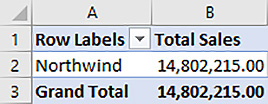
Another way to test security if you are a member of the server administrator role is to use one of the following connection string properties:

EffectiveUserName Use this property with a Windows domain user name like this: EffectiveUserName=DomainNameUserName.

Roles Use this property with one or more role names like this: Roles=Role1,Role2.

As an example, you can use the Roles property to test security in SSMS by opening a new MDX query window from the toolbar and then, in the Connect To Analysis Services dialog box, click Options, select the Additional Connection Parameters tab, and then type the connection string, as shown in Figure 2-28. Note that security does not affect the metadata pane in SSMS, so you can see all tables and dimensions. However, if you were to write a query to retrieve values from the Brand column, the results are correctly filtered.

You can also use this technique in client applications such as Excel by editing the connection string. For example, create a new workbook in Excel. On the Data tab of the ribbon, click From Other Sources, and then click From Analysis Services. On the Connect To Database Server of the Data Connection Wizard, type the server name (and instance name if required), and click Next. On the Select Database And Table page of the wizard, select the database containing your tabular model. If you are testing roles for a workspace version of your model rather than the deployed version, be sure to select the database with a GUID string appended to the database name in the drop-down list, select Model, and click Finish. Click OK in the Import Data dialog box. Then set up a PivotTable that includes a field in the columns or rows that you want to test.

Initially, you should see all data because your credentials allow you to see the unfiltered model. To test row-level security by using a connection string property, such as Roles, click Connections on the Data tab of the ribbon, click Properties, and append a semicolon and the connection string property to the connection string on the Definition tab, as shown in Figure 2-29. Click OK, click Yes to confirm the change to the connection string, and then click Close. The PivotTable should now be filtered.

One dynamic security option is to use the USERNAME function to get the Windows login for the user connecting to the model. This approach is preferred when users connect directly to a tabular model and can see or change the connection string used to make the connection. To do this, perform the following steps:

1. Create a permissions table in a relational database, such as the SalesTerritoryPermissions table shown in Table 2-12, to map user logins (assuming a domain name of WWI) to a filter value for the Sales Territory column in the City table. If a user can see multiple values, add multiple rows to the table.

Add the table to the model in SSDT by clicking Import From Data Source on the Model menu and using the Table Import Wizard to get data from the SalesTerritoryPermissions table.

2. Prevent users from viewing data in this table by right-clicking the table’s tab and clicking Hide From Client Tools.

3. Your next step is to create a role in the model, named SalesTerritoryRole for example. Give the role Read permissions, and ensure the users listed in the SalesTerritoryPermissions table are assigned to this role.

4. Next, define a row filter for the City table using the USERNAME function in an expression like this:

Click here to view code image

=CONTAINS(
    SalesTerritoryPermissions,
    SalesTerritoryPermissions[UserLogin],
    USERNAME(),
    SalesTerritoryPermissions[FilterValue],
    City[Sales Territory]
)

The first argument in the CONTAINS function specifies the table to evaluate and the next two arguments specify the column to check, and the value to look for in that column. Similarly, the fourth and fifth arguments are a column/value pair to evaluate. When the values in each column/value pair are found in the respective columns, the expression evaluates as TRUE. In other words, the current user can see sales territories when the UserLogin column of the SalesTerritoryPermissions table contains his or her login, and the FilterValue column in corresponding rows in the same table contains a sales territory.

5. You can test the dynamic security in SSMS by opening a new MDX query window, connecting to the tabular instance, and adding the following connection string properties to the Additional Connection Parameters page of the Connect To Analysis Services dialog box:

Click here to view code image

Roles=SalesTerritoryRole; EffectiveUserName=WWIEthan

6. After you successfully connect to the SSAS server and your model, run the following query to confirm the filter is applied correctly:

EVALUATE City

Another dynamic security option is to pass information about the current user in the CustomData property in the connection string. To do this, use the CUSTOMDATA function to access that property value and apply it as part of a row filter expression. This option is best when you have a custom client application that queries the tabular model on behalf of the users and users cannot view or modify the connection string.

Let’s say you set up a role called CustomSalesTerritory and use the following DAX expression as a row filter:

Click here to view code image

=IF(
    CUSTOMDATA()= "",
    FALSE(),
    City[Sales Territory] = CUSTOMDATA()
)

As with the previous examples, you can test this role in SSMS by opening a new MDX query window, connecting to the tabular instance, and adding the following connection string properties to the Additional Connection Parameters page of the Connect To Analysis Services dialog box:

Click here to view code image

Roles=CustomSalesTerritory; CustomData=Far West

And then in the query window, execute the following query to confirm the filter works:

EVALUATE City

SQL Server 2008 or later

Azure SQL Database

Azure SQL Data Warehouse

Analytics Platform System (formerly Parallel Data Warehouse)

Oracle 9i, 10g, 11g, and 12g

Teradata V2R6, V2

Implementing a tabular model in DirectQuery mode also has the following limitations:

You cannot create calculated tables in the model, nor can you add a pasted table. A workaround is to use corresponding logic to create a derived column or a view in the underlying source.

Some DAX functions do not translate correctly into SQL, particularly time-intelligence functions and some statistical functions. For these functions, consider adding a derived column in the underlying table instead.

Unlike ROLAP in a multidimensional model, DirectQuery does not cache query results within SSAS. If any caching occurs as a result of a query to a tabular model in DirectQuery mode, it happens only in the relational data source.

You can return only one million rows in a query. However, you can override this limitation by adding the MaxIntermediateRowSize property to the Msmdsrv.ini file.

Even if you create a tabular model in in-memory mode, you can always switch to DirectQuery mode at any time. If you do this, any data previously stored in the cache is flushed, but the metadata is retained. That means any measures, calculated columns, or property settings that you have added to the model are kept in the model.

If you start designing a tabular model by using in-memory storage and later decide to switch it to DirectQuery mode, you can encounter errors that must be resolved before you can complete the conversion. For example, you cannot convert a tabular model to DirectQuery mode if it contains multiple data source connections. You must first delete tables associated with the additional data sources, and then remove the data sources by clicking Existing Connections on the Model menu, selecting the data source connection in the Existing Connections dialog box, and clicking Delete. Click Close after all deleting the data sources.

Another obstacle to converting a tabular model to DirectQuery mode is the existence of a table in your model that is defined with multiple partitions. To fix this problem, click Partitions on the Table menu, select the partition in the Partition Manager, and click Delete. Repeat until you have only one partition for the table.

Regardless of the underlying data source, you have the following options for modeling when using DirectQuery mode:

Use all data, which is the only option in earlier versions of SQL Server.

Use no data, which is the new default.

Use a subset of data based on a query that you supply.

Even when using DirectQuery mode, you continue to use the Table Import Wizard to define and connect to your data source. When working with an empty tabular model, launch the wizard by selecting Import From Data Source from the Model menu. You select a relational database and then the tables for your model, but the wizard does not import the data. Instead, you work with an empty model that contains only metadata, such as column names and relationships, as shown in Figure 2-30. You perform all the same steps by configuring properties for columns, defining relationships, or working with the model in diagram view, but cannot view the results of your work as you can if you were to import data for an in-memory tabular model.

By working without the data, you can often perform modeling tasks faster because you no longer wait for calculations to complete after adding or changing measures or calculated columns. On the other hand, you can find it challenging to determine the effect of your modeling changes without viewing the data. In that case, you can import a subset of sample data that provides a view of these changes on a limited number of rows. This approach performs calculations faster than possible when working with the full set of underlying data.

To set up sample data, perform the following steps:

1. Click a table in the model designer, and then click Partitions on the Table menu.

2. Select the existing partition, which has the prefix (DirectQuery), click Copy, and then click the Query Editor button to add a WHERE clause to the partition query, and return a subset of the original partition query. For example, you can modify the query for the Sale table as shown in Figure 2-31.

When you add a sample partition definition like this, the Partition Manager includes a Set As DirectQuery button that appears only when you select a sample partition in the partition list. When you click this button, you reset the partition that Analysis Services uses to retrieve data for user queries. There can be only one DirectQuery partition defined for a table at any time. If you select the DirectQuery partition, the button’s caption displays Set As Sample instead. Although you can define only one DirectQuery partition, you can define multiple sample partitions.

3. When you close the Partition Manager, you must process the partition to load data into the sample partition. On the Model menu, point to Process, click Process Table, and click Close to close the Data Processing dialog box. The subset of rows defined by your query is displayed in the model designer, as shown in Figure 2-32.

The sample data partition is also accessible when you use the Analyze Table In Excel feature to test the model from the presentation layer. Using the sample partition makes it easier to test the results of calculations in measures, and to check relationships between tables even when you are using only a subset of data. Try this out by clicking Analyze In Excel on the Model menu. Notice the Analyze In Excel dialog box now requires you to choose one of two options, Sample Data View or Full Data View, as shown in Figure 2-33.

If you create sample partitions for some, but not all, tables in your model, and use the Analyze In Excel feature, you see only null values for columns in tables without a sample partition. Therefore, if you define a sample partition in one table, you should repeat the process for other tables. Your sample partition does not need to be a subset of the table. If the table is small, you can copy the DirectQuery partition and keep the existing query without adding a WHERE clause.

If you need to troubleshoot queries generated from your client application when using Oracle or Teradata as a source for your DirectQuery-mode tabular model, use the applicable trace monitoring tools for your source database instead of using Extended Events or SQL Profiler as you would for a SQL Server data source.

In Excel PivotTables, the standard method of the PivotTable Fields List to add items to rows, columns, and filters generates the appropriate MDX. However, you cannot use the Create Set Based On Row Items or Manage Sets commands, both of which are accessible by clicking Fields, Items, & Sets in the Calculations group of the Analyze tab on the ribbon. These commands are useful for building MDX sets at query time, which means they are session-scoped MDX statements and not supported by DirectQuery. This limitation is not exclusive to Excel; DirectQuery itself does not support any session-scoped constructs in ad hoc queries such as named sets, calculated members, calculated cells, visual totals, and default members.

DirectQueryMode=DirectQuery

After loading data into the model, you can enhance the model by adding measures to compute aggregate values, defining relationships to enable cross-filtering of data across tables, and creating hierarchies to provide users with a navigation path from summary to detail data. Optionally, you can separate data in a table into different partitions to manage the refresh process more efficiently. You can also add perspectives to focus the user on a subset of tables, hierarchies, or columns when the tabular model contains many objects. Another common tabular model enhancement is the addition of calculated columns to resolve data quality issues, concatenate columns values, or combine columns from related tables in preparation for building a hierarchy, to name a few reasons.

One new feature in SQL Server 2016 is the ability to create a calculated table. One reason you can do this is to add a time (or date) table to the tabular model when you do not have an existing table in your data source. To use DAX time intelligence functions, you must have a date table in your model. You can easily build a calculated date table by using the CALENDAR or CALENDARAUTO functions.

When you are ready for users to access the tabular model, you can publish it from SSDT by clicking Deploy on the Build menu or by right-clicking the project in Solution Explorer and clicking Deploy.

Tabular model development can begin in a desktop environment by using PowerPivot in Excel. You can then create a new project in SSDT by using the Import From PowerPivot template to load the PowerPivot workbook and import design into a tabular model.

When you deploy a tabular model from SSDT, you can configure the Processing Option and Transactional Deployment options when the model is set to compatibility level 1200. The Processing Option specifies the type of processing operation that SSAS should perform when deployment is complete, if any. The Transactional Deployment option determines whether deployment rolls back if the processing operation is not successful. When the tabular model is set to a lower compatibility level, you can also set the Query Mode option to DirectQuery, DirectQuery With In-Memory, In-Memory, or In-Memory With DirectQuery.

SSAS supports two storage modes for tabular models: in-memory and DirectQuery. You must refresh an in-memory tabular model by performing a processing operation periodically if you want to update the data in the model. A DirectQuery-mode tabular model does not require processing because it retrieves data from the underlying data source at query time and is thereby always up-to-date. There are several different types of processing operations: Process Add, Process Clear, Process Data, Process Default, Process Defrag, Process Full, and Process Recalc. You can use many of these operations at the database, table, or partition level, but some operations are restricted to specific levels. Furthermore, you should understand how they each affect memory resources and dependent objects.

You can convert an in-memory tabular model to DirectQuery mode as long as the model has a single supported data source and only the default partition defined for each table. You have the option to configure constrained delegation if you want to pass user credentials to the backend database at query time.

You can schedule the refresh of data in several ways. A straightforward option is to script the processing operation as TMSL and then add the script as a job step in a scheduled SQL Server Agent job. Other options include using SSIS, AMO, or PowerShell.

Security for a tabular model is role-based and requires you to assign Windows logins or groups to a role to enable access. You can assign users to a server administrative role to enable full access to all objects and all tasks on the SSAS server. Most of the time, you assign users to a database role to restrict them to administrative tasks or read activities on a specific database. You can restrict users to a specific set of data in the tabular model by implementing row-level security, which requires you to define a filter by using a DAX expression.

DirectQuery enables you to build a tabular model that accesses data directly from the backend database in near real-time, although some limitations exist that you should be able to enumerate. In previous versions of SQL Server, DirectQuery could retrieve data only from SQL Server databases. Beginning with SQL Server 2016, you can now use any of the following data sources: Azure SQL Database, Azure SQL Data Warehouse, Analytics Platform System, Oracle, and Teradata. While you design your DirectQuery-mode tabular model, you can choose to perform your modeling tasks with all data, some data, or no data. You can check your work by defining a partition for sample data and then using an Excel PivotTable to query the model. A PivotTable generates MDX, which is now supported by DirectQuery and translated into platform-specific SQL for the backend database.

Use the DirectQueryMode=DirectQuery connection parameter in the connection string of a tool that supports access to a tabular model at compatibility level 1100 or 1103 with its Query Mode set to In-Memory With DirectQuery when you want to convert an in-memory query to DirectQuery.

Wingtip Toys is a company that has two channels for sales, Internet, and Direct Sales. The company sells toys to individual consumers on a commercial website. They also sell to companies by using a direct sales teams located in branch offices in key regions worldwide.

As part of your role as a BI developer at Wingtip Toys, you are responsible for developing and implementing a SSAS tabular model set to compatibility level 1200 to meet a specific set of business requirements.

The current database environment includes two OLTP systems that run on separate instances of SQL Server 2016, set up with Availability Groups. To protect the OLTP systems, you source the data from read-only secondary replicas. The data you need for the tabular model is found in following the tables and columns listed for each database:

Database: WingtipWebSales

Sales: Invoice Date, CustomerID, ProductID, SaleAmount, Quantity

Customer: CustomerID, FirstName, LastName, EmailAddress, StreetAddress, City, StateProvince, Country, PostalCode

Product: ProductID, ProductName, Brand, Size, Color, Dimensions, Description, UnitPrice

Database: WingtipDirectSales

Sales: InvoiceDate, CustomerID, ProductID, SalespersonID, TotalAmount, UnitsSold

Customer: CustomerID, CompanyName, StreetAddress, City, StateProvince, Country, PostalCode, ContactName, PhoneNumber

Salesperson: SalespersonID, FirstName, LastName, Login, City, SalesTerritoryID

Sales Territory: SalesTerritoryID, Sales Territory, Country, Region

Product: ProductID, ProductName, Brand, Size, Color, Dimensions, Description, UnitPrice

Users plan to use Excel 2016 to answer the following types of questions:

What are total sales and total quantities sold by date, product, sales territory, sales person, customer, and sales channel?

How many Internet sales transactions occur hourly each day?

To satisfy the business requirements, the tabular model must have the following characteristics:

The Internet sales information must be available in near real-time.

The Internet sales team must be restricted to viewing sales data from the WingtipSales database only.

Each salesperson must be restricted to viewing sales data for the sales territory to which he or she is assigned.

Management must be able to view all sales data.

The salesperson table must support drilling from region to country to city to salesperson.

The model must support analyzing sales by dates.

Based on this background information and business requirements, answer the following questions:

1. Which of the following steps do you need to perform to enable management to view Total Sales for both sales channels combined?

A. Create a linked server on one of the SQL Server instances to enable access to the other instance.

B. Use the Table Import Wizard to import data by creating a query to union the Sales tables from WingtipWebSales and WingtipDirectSales and rename the new table in the tabular model as Sales.

C. Use the Table Import Wizard to import data from the Sales tables in each database as separate tables, with one table named Internet Sales, and the other table named Direct Sales.

D. Create a measure named Total Sales in the Sales table by using a DAX expression to sum the values in the SaleAmount column and add it to the sum of the values in the Total Amount column.

E. Create a measure named Total Internet Sales in the Internet Sales table by using a DAX expression to sum the SaleAmount column.

F. Create a measure named Total Direct Sales in the Direct Sales table by using a DAX expression to sum the TotalAmount column.

G. Create a measure in either the Total Direct Sales or Total Internet Sales table by using a DAX expression to add Total Direct Sales to Total Internet Sales.

2. Which of the following steps do you need to perform to create the Sales Territory hierarchy?

A. Switch to Diagram view in the model designer and create a many to one relationship between the Sales Territory and Salesperson tables, if necessary.

B. Right-click the Sales Territory table, and click Create Hierarchy.

C. Right-click the Salesperson table, and click Create Hierarchy.

D. Type Sales Territory as the hierarchy name.

E. Create the Salesperson calculated column in the Salesperson table by concatenating FirstName and LastName.

F. Create the following calculated columns in the Sales Territory table by using the RELATED function: City, Salesperson.

G. Create calculated columns in the Salesperson table by using the RELATED function: Region, Country.

H. Right-click the following columns in the Sales Territory table, point to Add To Hierarchy, and click Sales Territory: Region, Country, City, Salesperson.

I. Right-click the following columns in the Salesperson table, point to Add To Hierarchy, and click Sales Territory: Region, Country, City, Salesperson.

3. What type of partitioning strategy should you implement to support the analysis of hourly Internet sales transactions?

A. Create one partition per hour per day dynamically by running an SSIS package each hour to build the new partition. Load the data for the current hour by performing a Process Add, and then execute a Process Recalc on the partition.

B. Create one partition per day dynamically by running an SSIS package daily to build the new partition. Load the data for the current day by performing a Process Full operation on the partition.

C. Set the model to DirectQuery With In-Memory Mode. Define a sample partition for the Internet Sales table to view data during development.

D. Convert the model to DirectQuery. Add columnstore indexes to the source tables. In the model, define a sample partition for all tables to view data during development.

4. How can you enhance the model to support analysis by date?

A. Create calculated columns in the Internet Sales and Direct Sales tables to derive year, quarter, and month from the InvoiceDate columns.

B. Create a calculated table using the CALENDARAUTO function and add calculated columns to the calculated table to derive year, quarter, and month from the InvoiceDate columns.

C. Create a date table in a new SQL Server database, and import it into the model by using the Table Import Wizard.

D. Create a calculated column in the Internet Sales and Direct Sales tables using the CALENDAR function on the InvoiceDate column.

5. Which is the easiest option for configuring and maintaining security for each salesperson?

A. Create a role for each salesperson with a row filter restricting the user to a specific sales territory in the Direct Sales table.

B. Create one role for the salesperson group with a row filter on the Direct Sales table that uses the CUSTOMDATA function.

C. Create a one role for the salesperson group with a row filter on the Direct Sales table that uses the CONTAINS and USERNAME functions to find the user’s sales territory in the Salesperson table.

D. Create a permissions table, add it to the tabular model, and define a relationship between it and the Direct Sales table.

6. The project’s Processing Option property is set to Do Not Process. You add a Total Quantity as a new measure to the Direct Sales table in the tabular model in SSDT and deploy the model. Based on your answer to Question 3, how do you ensure users can use the new measure in the deployed model?

A. Open SSMS, open the Tables folder for the model’s database, right-click the Direct Sales table, click Process Table, and select Process Recalc in the Mode drop-down list.

B. Nothing. The new measure is deployed and accessible without processing because the model is in DirectQuery mode.

C. Open SSMS, right-click the database containing your model, and click Process Database.

D. Open SSMS, open the Tables folder for the model’s database, right-click the Direct Sales table, click Process Table, and select Process Default in the Mode drop-down list.

1. The answers are C, E, F, G. The ideal way to design the model is to import the two sales tables separately to satisfy the data access requirements for each sales channel, create separate measures for each channel, and then add these two measures together for total sales.

Answer A is unnecessary because the tables should be imported separately and separate data connections to the source directly do not require a linked server. Answers B and D are incorrect due to the security requirements. Although a row filter could be used to isolate each channel type, the performance of a row filter on large tables containing sales data is not optimal when separate tables suffice.

2. The answers are A, C, D, E, G, I. The Salesperson table must contain the hierarchy because it contains Salesperson column, which is created as a calculated column by concatenating FirstName and LastName. You must create calculated columns by using the RELATED function to include the Region and Country columns in the Salesperson table.

Answers B and H are incorrect because the Sales Territory table does not contain the column for the lowest level of the hierarchy. Answer F is also incorrect because it is not possible to use the RELATED function in the table on the many side of the many-to-one relationship.

3. The answer is D. The near real-time requirement for Internet Sales means the model must be set to DirectQuery. Because the compatibility level is set to 1200, the entire model must be in DirectQuery mode.

Answers A and B do not satisfy the near-real time requirement. Answer C is not correct because DirectQuery With In-Memory Mode is not available when the compatibility level is 1200.

4. The answer is C. Of the four possible answers, only C is correct. It can be as simple or as complex as you need.

Answer A is incorrect. Although the addition of calculated columns for dates in the two sales tables is adequate when a user interacts only with one of the sales table due to security requirements, it is not a suitable solution for management users who want to see data from both tables at the same time. For this scenario, a separate table enables time analysis across all sales data. Answer B is incorrect because the model is in DirectQuery mode (see Question 3) and calculated tables are not supported. Answer D is incorrect because the CALENDAR function returns a table and therefore cannot be used to create a calculated column.

5. The answer is C. The Salesperson table has the information necessary to develop a DAX expression that uses the CONTAINS function to find the user’s sales territory by matching the USERNAME to a sales territory. A single role can be defined in the model with a row filter and then all other maintenance takes place in the Salesperson table as salesperson rows are added or removed or the sales territories are changed as a normal part of business operations.

Answer A is incorrect because it requires too much maintenance to require a separate role for each salesperson. Answer B is incorrect because the CUSTOMDATA function requires you to have another mechanism determine what value to pass in the function, typically as part of a custom application. Answer D is incorrect because the existence of a permissions table with a relationship to the Direct Sales table is insufficient. A role must be defined to determine how the permissions table is used to secure access to the Direct Sales table.

6. The answer is B. No processing is required when you deploy a DirectQuery model.

Answers A, C, and D are incorrect because process operations are not supported by DirectQuery.