
Computers can only perform finite computations. Consequently, computers only make use of finite precision representations of numbers. This has several important implications in the context of scientific computation.
This chapter provides an overview of the representations and properties of values of types int and float, used to represent members of the sets Z and R, respectively. Practical examples demonstrating the robust use of floating-point arithmetic are then given. Finally, some other forms of arithmetic are discussed.
In this section, we shall introduce the representation of integer and floating-point numbers before outlining some properties of these representations.
Positive integers are represented by several, least-significant binary digits (bits). For example, the number 1 is represented by the bits ... 00001 and the number 11 is represented by the bits ... 01011. Negative integers are represented in twoscomplement format. For example, the number −1 is represented by the bits ... 11111 and the number −11 is represented by the bits ... 10101.
![Values i of the type int, called machine-precision integers, are an exact representation of a consecutive subset of the set of integers i ϵ [I... u] C Z where I and u are given by min_int and max_int, respectively.](http://imgdetail.ebookreading.net/software_development/33/9780470242117/9780470242117__f-for-scientists__9780470242117__figs__0401.png)
Figure 4.1. Values i of the type int, called machine-precision integers, are an exact representation of a consecutive subset of the set of integers i ϵ [I... u] C Z where I and u are given by min_int and max_int, respectively.
Consequently, the representation of integers n ϵ Z by values of the type int is exact within a finite range of integers (illustrated in figure 4.1). This range is platform specific and may be obtained as the min_int and max_int values. On a 32-bit platform, the range of representable integers is substantial:
> min_int, max_int;;
val it : int * int = (-2147483648, 2147483647)
On a 64-bit platform, the range is even larger.
The binary representation of a value of type int may be obtained using the following function:
> let binary_of_int n =
    [for i in Sys.word_size - 1 .. −1 .. 0 ->
       if (n>>>i) %2 = 0 then "0" else "1"]
    |> String.concat "";;
val binary_of_int : int -> string
For example, the 32-bit binary representations of 11 and — 11 are:
> binary_of_int 11;;
val it : string = "0000000000000000000000000001011"

> binary_of_int (-11);;
val it : string = "1111111111111111111111111110101"
As we shall see in this chapter, the exactness of the int type can be used in many ways.
In science, many important numbers are written in scientific notation. For example, Avogadro's number is conventionally written NA = 6.02214 × 10²³. This notation essentially specifies the two most important quantities about such a number:
the most significant digits called the mantissa, in this case 6.02214, and
the offset of the decimal point called the exponent, in this case 23.
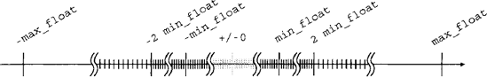
Figure 4.2. Values of the type float, called double-precision floating-point numbers, are an approximate representation of real-valued numbers, showing: a) full-precision (normalized) numbers (black), and b) denormalized numbers (gray).
Computers use a similar, finite representation called "floating point" which also contains a mantissa and exponent. In F#, floating-point numbers are represented by values of the type float. Roughly speaking, values of type int approximate real numbers between min_int and max_int with a constant absolute error of ±½ whereas values of the type float have an approximately-constant relative error that is a tiny fraction of a percent.
In order to enter floating-point numbers succinctly, the F# language uses a standard "e" notation, equivalent to scientific number notation a × 10b. For example, the number 5.4 × 10¹² may be represented by the value:
> 6.02214e23;;
val it : float = 6.02214e+23
As the name "floating point" implies, the use of a mantissa and an exponent allows the point to be "floated" to any of a wide range of offsets. Naturally, this format uses base-two (binary) rather than base-ten (decimal) and, hence, numbers are represented by the form a × 2b where a is the mantissa and b is the exponent. Double-precision floating-point values consume 64-bits, of which 53 bits are attributed to the mantissa (including one bit for the sign of the number) and the remaining 11 bits to the exponent.
By default, F# interactive mode only displays a few digits of precision. In order to examine floating point numbers more accurately from the interactive mode, we shall replace the pretty printer used to visualize values of the float type with one that conveys more precision:
> fsi.AddPrinter(sprintf "%0.2 0g");;
val it : unit = ()
Compared to the type int, the exponent in a value of type float allows a huge range of real-valued numbers to be approximated. As for the type int, this range is given by the predefined values:
> min_float, max_float;;
val it : float * float =
  (2.22507385850720138e-308, 1.79769313486231571e+308)
Some useful values not in the set of real numbers R are also representable in floating-point number representation. Numbers out of range are expressed by the values -0.0, - Infinity (-∞) and Infinity (∞). For example, in floatingpoint arithmetic
> 1.0 / 0.0;;
val it : float = Infinity
Floating point arithmetic includes a special value denoted nan in F# that is used to represent results that are "not a number". This is used when calculations do not return a real-valued number x ϵ R, e.g. when a supplied parameter falls outside the domain of a function. For example[16], ln(—1) ∉ R:
> log −1.0; ,-
val it : float = NaN
The domain of the log function is 0 ≤ x ≤ ∞, with log 0.0 evaluating to -Infinity,and log infinity evaluating to infinity.
The special value nan has some interesting and important properties. In particular, all comparisons involving nan return false except inequality of nan with itself:
> nan < = 3.0;;
val it : bool = false

> nan >= 3.0;;
val it : bool = false

> nan <> nan;;
val it : bool = true
However, although comparing nan with itself using equality indicates that nan is not equal to itself, the built-in compare function returns 0 when comparing nan with nan as a special case:
> compare nan nan;;
val it : int = 0
This ensures that collections built using the compare function, such as sets (described in section 3.4), do not leak when many nan values are inserted:
> set [nan; nan; nan];;
val it : Set<float> = seq [NaN]
In the case of ln(-l), the implementation of complex numbers provided in the Math. Complex module may be used to calculate the complex-valued result ln(—1) = πi:
> log(complex −1.0 0.0);;
val it : Complex = 0.Or + 3.141592654i
Note that the built-in log function is overloaded to work transparently on the complex type as well as the float type. This makes it very easy to write functions that handle complex numbers in F#.
As well as min_float, max_float, infinity and nan, F# also predefines contains an epsilon_float value:
> epsilon_f loat;;
val it : float = 2.22044604925031308e-16
This is the smallest number that, when added to one, does not give one:
> 1.0 + epsilon_float;;
val it : float = 1.00000000000000022
Consequently, the epsilon_float value is seen in the context of numerical algorithms as it encodes the accuracy of the mantissa in the floating point representation. In particular, the square root of this number often appears as the accuracy of numerical approximants computed using linear approximations (leaving quadratics terms as the largest remaining source of error). This still leaves a substantially accurate result, suitable for most computations:
> 1.0 + sqrt epsilon_float;;
val it : float = 1.000000015
This was used in the definition of the d combinator in section 1.6.4.
The approximate nature of floating-point computations is often seen in simple calculations. For example, the evaluation of
> 1.0 / 3.0;;
val it : float = 0.333333333333333315
In particular, the binary representation of floating-point numbers renders many decimal fractions approximate. For example, although 1 is represented exactly by the type float, the decimal fraction 0.9 is not:
> 1.0 - 0.9;;
val it : float = 0.0999999999999999778
Many of the properties of conventional algebra over real-valued numbers can no longer be relied upon when floating-point numbers are used as a representation. For more details, see the relevant literature [17].
In real arithmetic, addition is associative:
In general, this is not true in floating-point arithmetic. For example, in floatingpoint arithmetic (0.1 + 0.2) + 0.3 ≠ 0.1 + (0.2 + 0.3):
> (0.1 + 0.2) + 0.3 = 0.1 + (0.2 + 0.3);;
val it : bool = false
In this case, round-off error results in slightly different approximations to the exact answer that are not exactly equal:
> (0.1 + 0.2) + 0.3, 0.1 + (0.2 + 0.3);;
val it : float * float =
  (0.60000000000000009, 0.59999999999999998)
Hence, even in seemingly simple calculations, values of type float should not be compared for exact equality.
More significant errors are obtained when dealing with the addition and subtraction of numbers with wildly different exponents. For example, in real arithmetic 1.3 + 1015 - 1015 = 1.3 but in the case of float arithmetic:
> 1.3 + lel5 - lel5;;
val it : float =1.25
The accuracy of this computation is limited by the accuracy of the largest magnitude numbers in the sum. In this case, these numbers are 1015 and −1015, resulting in a significant error of 0.05 in this case.
In general, this problem boils down to the subtraction of similar-sized numbers. This includes adding a similar-sized number of the opposite sign.
The accuracy of calculations performed using floating-point arithmetic may often be improved by carefully rearranging expressions. Such rearrangements often result in more complicated expressions which are, therefore, slower to execute.
Consider the following function f(x):
This involves the subtraction of a pair of similar numbers when x ≃ 0. This may be expressed in F# as:
> let f_l x =
    sqrt (1.0 + x) - 1.0;;
val f_l : float -> float
As expected, results of this function are significantly erroneous in the region x ≃ 0. For example:

> f_l le-15;;
val it : float = 4 .4408920985006262e-16
Note that the result given by F# differs from the mathematical result by ~ 0.056. The /i function may be rearranged into a form which evades the subtraction of similar-sized numbers around x ≃ 0:
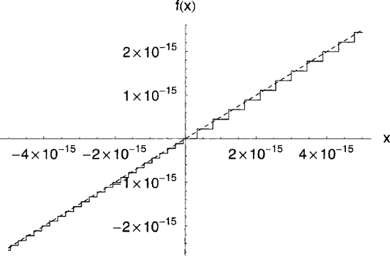
Figure 4.3. Accuracy of two equivalent expressions when evaluated using floating-point arithmetic: a)
This alternative definition may be expressed in F# as:
> let f_2 x =
    x / (1.0 + sqrt (1.0 + x));;
val f_2 : float -> float
Although f1(x) = f2(x) ∀ x ϵ R, the f2 form of the function is better behaved when evaluated in the region x ≃ 0 using floating-point arithmetic. For example, the value ofthe function at x = 10−15 is much better approximated by f2 than it was by f1:
> f_2 le-15;;
val it : float = 4.9999999999999994e-16
This is particularly clear on a graph ofthe two functions around x ≃ 0 (illustrated in figure 4.3).
Due to the accumulation of round-off error, loops should not use loop variables of type float but, rather, use the type int and, if necessary, convert to the type float within the loop. Interpolation is an important example of this.
Comprehensions provide an easy way to demonstrate this. The following comprehension generates a list of values interpolating from 0.1 to 0.9 inclusive:
> [0.1 .. 0.2 .. 0.9];;
val it : float list = [0.1; 0.3; 0.5; 0.7; 0.9]
However, specifying the step size in this way is not numerically stable because repeated float additions lead to numerical error. For example, using a step size of 0.16 leads to the last value being omitted:
> [0.1 . . 0.16 . . 0.9];;
val it : float list = [0.1; 0.26; 0.42; 0.58; 0.74]
In this case, the result of repeatedly adding the approximate representation of d to that of x, starting with x = l, produced an approximation which was slightly greater than u. Thus, the sequence terminated too early. This produced a list containing five elements instead of the expected six.
As such functionality is commonly required in scientific computing, a robust alternative must be found.
Fortunately, this problem is easily solved by resorting to an exact form of arithmetic for the loop variable, typically int arithmetic, and converting to floating-point representation at a later stage. For example, the interp function may be written robustly by using an integer loop variable i:
for i ϵ {1... n}:
> let interp xl xn n =
    [for i in 1 .. n ->
       xl + float(i - 1) * (xn - xl) / float(n - 1)];;
val interp : float -> float -> int -> float list
Thanks to the use of an exact form of arithmetic, this function produces the desired result:
> interp 0.1 0.9 6;;
val it : float list = [0.1; 0.26; 0.42; 0.58; 0.74; 0.9]
In terms of comprehensions, this is equivalent to:
> [for i in 0 .. 5 ->
     0.1 + float i * 0.8 / 5.0];;
val it : float list = [0.1; 0.26; 0.42; 0.58; 0.74; 0.9]
We shall now conclude this chapter with two simple examples of the inaccuracy of floating-point arithmetic.
The solutions of the quadratic equation ax2 + bx + c = 0 are well known to be:
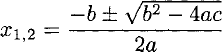
The root
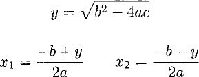
These values are easily calculated using floating-point arithmetic:
> let quadratic a b c =
    let y = sqrt (b*b-4.0*a*c)
    (-b + y) / (2.0 * a), (-b - y) / (2.0 * a);;
val quadratic : float -> float -> float -> float * float
However, when evaluated using floating-point arithmetic, these expressions can be problematic. Specifically, when b2 >> 4ac, subtracting 4ac from b2 in the subexpression b2 — 4ac will produce an inaccurate result approximately equal to b2. This results in
For example, using the conditions a = 1, b = 109 and c = 1, the correct solutions are x ≃ —10−9 and —109 but the above implementation of the quadratic function rounds the smaller magnitude solution to zero:
> quadratic 1.0 le9 1.0;;
val it : float * float = (0.0, -le+9)
The accuracy of the smaller-magnitude solution is most easily improved by calculating the smaller-magnitude solution in terms of the larger-magnitude solution, as:
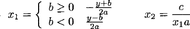
This formulation, which avoids the subtraction of similar values, may be written:
> let quadratic a b c =
    let y = sqrt (b*b-4.0*a*c)
    let xl = (if b < 0.0 then y-b else -y-b) / (2.0 * a)
    xl, c / (xl * a);;
val quadratic : float -> float -> float -> float * float
This form of the quadratic function is numerically robust, producing a more accurate approximation for the previous example:
> quadratic 1.0 le9 1.0;;
val it : float * float = (-1000000000.0, -le-09)
Numerical robustness is required in a wide variety of algorithms. We shall now consider the evaluation of some simple quantities from statistics.
In this section, we shall illustrate the importance of numerical stability using expressions for the mean and variance of a set of numbers.
The mean value
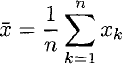
The sum may be computed by folding addition over the elements and dividing by the length:
> let mean xs =
    Seq.fold (+) 0.0 xs / float(Seq.length xs);;
val mean : #seq<float> -> float
Note that this definition of the mean function can be applied to any sequence container (lists, arrays, sets etc.).
For example, the mean of
> mean [|1. 0; 3.0; 5.0; 7 . 0 |];;
val it : float =4.0
Although the sum of a list of floating point numbers may be computed more accurately by accumulating numbers at different scales and then summing the result starting fromthe smallest scale numbers, the straightforward algorithm used by this mean function is often satisfactory. The same cannot be said of the straightforward computation of variance.
The variance σ2 of a set Xk of numbers is typically written:
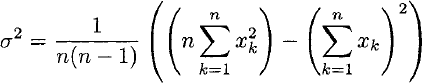
Although variance is a strictly non-negative quantity, the subtraction of the sums in this expression for the variance may produce small, negative results when computed directly using floating-point arithmetic, due to the accumulation of rounding errors. This problem can be avoided by computing a numerically robust recurrence relation [17]:
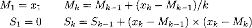
Thus, the variance may be computed more accurately using the following functions:
> let variance_aux (m, s, k) x =
    let m' = m + (x - m) / k
m', s + (x - m) * (x - m') , k + 1.0;;
val variance_aux :
float * float * float -> float ->
float * float * float
> let variance xs =
let _, s, n2 = Seq.fold aux (0.0, 0.0, 1.0) xs
S / (n2 - 2.0);;
val variance : #seq<float> -> floatThe auxiliary function variance_aux accumulates the recurrence relation when it is folded. The variance function simply folds this auxiliary function over the sequence to return a better-behaved approximation to the variance
For example, the variance of
> variance [|1. 0; 3.0; 5.0; 7 . 0 |];;
val it : float = 6.66666666666666696
The numerical stability of this variance function allows us to write a function to compute the standard deviation σ the obvious way, without having to worry about negative roots:
> let standard_deviation x =
    sqrt (variance x);;
val variance : #seq<float> -> float
Clearly numerically stable algorithms which use floating-point arithmetic can be useful. We shall now examine some other forms of arithmetic.
As we have seen, the int and float types in F# represent numbers to a fixed, finite precision. Although computers can only perform arithmetic on finite-precision numbers, the precision allowed and used could be extended indefinitely. Such representations are known as arbitrary-precision numbers.
The vast majority of F# programs use machine-precision integer arithmetic (described in section 4.1.1) because it is provided in hardware and, consequently, is extremely efficient. In some cases, programs are required to handle integers outside the range of machine-precision integers. In such cases, F# programs can use the built-in Math. Biglnt type.
Arbitrary-precision integers may be specified as literals with an I suffix:
> open Math;;
> 123I;;
val it : bigint = 123I
The Bigint class provides some useful functions for manipulating arbitrary-precision integers such as a factorial function:
> Bigint.factorial 33I;;
val it : bignum = 8683317618811886495518194401280000000I
Arbitrary-precision integers are used in some parts of scientific computing, most notably in computer algebra systems.
Rationals, fractions of the form
Compared to the type float, rational arithmetic allows arbitrary precision to be used for any value in 3EL However, arithmetic operations on floating point numbers are 0 (1) but arithmetic operations on arbitrary-precision rational numbers are asymptotically slower. The larger the numerators and denominators, the slower the calculations.
Arbitrary-precision rational arithmetic is implemented by the BigNum class. Rational literals are written 123N or:
> 123N / 456N;;
val it : bignum = 41/152N
Note that the fraction is automatically reduced, in this case by dividing both numerator and denominator by 3.
For example, an arbitrary-precision factorial function may be written:
> let rec factorial = function
    | 0 -> 1N
    | n -> BigNum.of_int n * factorial (n - 1);;
val factorial : int -> bignum
> factorial 33;;
val it : bignum = 8683317618811886495518194401280000000N
Rational arithmetic, represented by the constructor Ratio, may then be used to calculate an approximation to:
> open Math;;

> let rec e = function
    | 0 -> IN
    | n -> IN / factorial n + e (n - 1);;
val e : int -> BigNum
For example, the first eighteen terms give the rational approximation to e of:
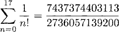
> e 17;;
val it : string = 7437374403113/2736057139200N
Converting this result from rational representation into a floating point number demonstrates that the result is very close to the value given by a native floating point evaluation of e:
> Math.BigNum.to_float(e 17);;
val it : float = 2.718281828

> exp 1.0;;
val it : float = 2.718281828
Rational arithmetic can be useful in many circumstances, including geometric computations.
Some problems can use ordinary precision floating-point arithmetic most of the time and resort to higher-precision arithmetic only when necessary. This leads to adaptive-precision arithmetic, which uses fast, ordinary arithmetic where possible and resorts to suitable higher-precision arithmetic only when required.
Geometric algorithms are an important class of such problems and a great deal of interesting work has been done on this subject [24]. This work is likely to be of relevance to scientists studying the geometrical properties of natural systems.
[16] Note that negative float literals do not need brackets, i.e. log -1.0 is equivalent to log (-1.0).