
Scientific applications are among the most computationally intensive programs in existence. This places enormous emphasis on the efficiency of such programs. However, much time can be wasted by optimizing fundamentally inefficient algorithms and concentrating on low-level optimizations when much more productive higher-level optimizations remain to be exploited.
Too commonly, a given problem is shoe-horned into using arrays because more sophisticated data structures are prohibitively complicated to implement in many common languages. Examples of this problem, endemic in scientific computing, are rife. For example, Finite element materials simulations, numerical differential equation solvers, numerical integration, implicit surface tesselation and simulations of particle or fluid dynamics based around uniformly subdivided arrays when they should be based upon adaptively subdivided trees.
Occasionally, the poor performance of these inappropriately-optimized programs even drives the use of alternative (often approximate) techniques. Examples of this include the use of padding to round vector sizes up to integer-powers of two when computing numerical Fourier transforms (Fourier series). In order to combat this folklore-based approach to optimization, we shall introduce a more formal approach to quantifying the efficiency of computations. This approach is well known in computer science as complexity theory.
The single most important choice determining the efficiency of a program are the selection of algorithms and of data structures. Before delving into the broad spectrum of data structures accessible from F#, we shall study the notion of algorithmic complexity. This concept quantifies algorithm efficiency and, therefore, is essential for the objective selection of algorithms and data structures based upon their performance. Studying algorithmic complexity is the first step towards drastically improving program performance.
In order to compare the efficiencies of algorithms meaningfully, the time requirements of an algorithm must first be quantified. Although it is theoretically possible to predict the exact time taken to perform many operations such an approach quickly becomes intractable.
Consequently, exactness can be productively relinquished in favour of an approximate but still quantitative measure of the time taken for an algorithm to execute. This approximation, the conventional notion of algorithmic complexity, is derived as an upper- or lower-bound or average-case[10] of the amount of computation required, measured in units of some suitably-chosen primitive operations. Furthermore, asymptotic algorithmic efficiency is derived by considering these forms in the limit of infinite algorithmic complexity.
We shall begin by describing the notion of the primitive operations of an algorithm before deriving a mathematical description for the asymptotic complexity of an algorithm. Finally, we shall demonstrate the usefulness of algorithmic complexity in the optimization of a simple function.
In order to derive an algorithmic complexity, it is necessary to begin by identifying some suitable primitive operations. The complexity of an algorithm is then measured as the total number of these primitive operations it performs. In order to obtain a complexity which reflects the time required to execute an algorithm, the primitive operations should ideally terminate after a constant amount of time. However, this restriction cannot be satisfied in practice (due to effectively-random interference from cache effects etc.), so primitive operations are typically chosen which terminate in a finite amount of time for any input, as close to a constant amount of time as possible.
For example, a first version of a function to raise a floating-point value x to a positive, integer power n may be implemented naïvely as:
> let rec ipow_l x = function
| 0 -> 1.0
    | n -> x * ipow_l x (n - 1);;
val ipow_l : float -> int -> float
The ipow_l function executes an algorithm described by this recurrence relation:
Consequently, this algorithm performs the floating-point multiply operation exactly n times in order to obtain its result, i.e. x° = 1, x1 = x x 1, x2 = x x x x 1 and so on. Thus, floating-point multiplication is a logical choice of primitive operation. Moreover, this function multiplies finite-precision numbers and the algorithms used to perform this operation in practice (which are almost always implemented as dedicated hardware) always perform a finite number of more primitive operations at the bit level, regardless of their input. Thus, this choice of primitive operation will execute in a finite time regardless of its input.
We shall now examine an approximate but practically very useful measure of algorithmic complexity before exploiting this notion in the optimization of the ipow_l function.
The complexity of an algorithm is the number of primitive operations it performs. For example, the complexity of the ipow_l function is T (n) = n.
As the complexity can be a strongly dependent function of the input, the mathematical derivation of the complexity quickly becomes intractable for reasonably complicated algorithms.
In practice, this is addressed in two different ways. The first approach is to derive the tightest possible bounds of the complexity. If such bounds cannot be obtained then the second approach is to derive bounds in the asymptotic limit of the complexity.
An easier-to-derive and still useful indicator of the performance of a function is its asymptotic algorithmic complexity. This gives the asymptotic performance of the function in the limit of infinite execution time.
Three notations exist for the asymptotic algorithmic complexity of a function f(x)
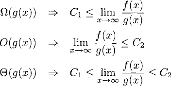
for some constants C1, C2 ϵ R.
The
The formulation of the asymptotic complexity of a function leads to some simple but powerful manipulations:
f(x) is O(ag(x)), a > 0 => f(n) is 0(g(x)), i.e. constant prefactors can be removed.
f(x) is 0(xa + xb), a > b > 0 => f(x) is 0(xa), i.e. the polynomial term with the largest exponent dominates all other polynomial terms.
f(x) is 0(xa + bx), a > 0, b > 0 => f(n) is 0(bx), i.e. exponential terms dominate any polynomial terms.
f (x) is 0{ax + bx), a > b > 0 =>f (n) is 0 (ax), i.e. the exponential term ax with the largest mantissa a dominates all other exponential terms.
These rules can be used to simplify an asymptotic complexity.
As the complexity of the ipow_l function is T (n) = n, the asymptotic complexities are clearly 0(n), Ω(n) and, therefore,
The algorithm behind the ipow_l function can be greatly improved upon by reducing the computation by a constant proportion at a time. In this case, this can be achieved by trying to halve n repeatedly, rather than decrementing it. The following recurrence relation describes such an approach:
> let rec ipow_2 x = function
| 0 -> 1.0
| 1 -> x
| n ->
let x2 = ipow_2 x (n/2)
x2 * if n mod 2=0 then x2 else x * x2;;
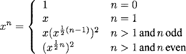
val ipow_2 : float -> int -> floatThis variant is clearly more efficient as it avoids the re-computation of previous results, e.g. x4 is factored into (x2)2 to use two floating-point multiplications instead of four. Quantifying exactly how much more efficient is suddenly a bit of a challenge!
We can begin by expanding the computation manually for some small n (see Table 3.1) as well as computing and plotting the exact number of integer multiplications performed for both algorithms as a function of n (shown in figure 3.1).
Table 3.1. Complexity of the ipow_ 2 function measured as the number of multiply operations performed.
n | Computation | T(n) |
0 | 1 | 0 |
1 | x | 0 |
2 | x × x2 | 1 |
3 | x × x2 | 2 |
4 | (x2)2 | 2 |
5 | x × (x2)2 | 3 |
6 | (x × x2)2 | 3 |
7 | x × (x × x2)2 | 4 |
8 | ((x2)2)2 | 3 |
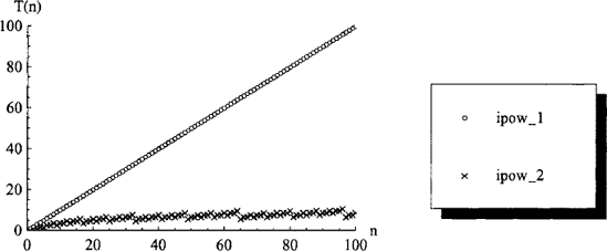
Figure 3.1. Complexities of the ipow_l and ipow_2 functions in terms of the number T(n) of multiplies performed.
Lower and upper bounds of the complexity can be derived by considering the minimum and maximum number of multiplies performed in the body of the ipow_2 function, and the minimum and maximum depths of recursion.
The minimum number of multiplies performed in the body of a single call to the ipow_2 function is 0 for n d 1, and 1 for n > 1. The function recursively halves n, giving a depth of recursion of 1 for n d 1, and at least [log2 n] for n > 1. Thus, a lower bound of the complexity is 0 for n d 1, and log2(n) — 1 for n > 1.
The maximum number of multiplies performed in the body of a single call to the ipow_2 function is 2. The depth of recursion is 1 for n d 1 and does not exceed [log2 n] for n > 1. Thus, an upper bound of the complexity is 0 for nd 1, and 2(1 +log2n) forn > 1.
From these lower and upper bounds, the asymptotic complexities of the ipow_2 function are clearly Ω(ln n), O (ln n) and, therefore,
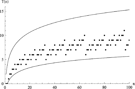
Figure 3.2. Complexities of the ipow_2 function in terms of the number of multiplies performed, showing: exact complexity T(n) (dots) and lower- and upper-bounds algorithmic complexities log2(n) — 1 ≤ T (n) ≤ 2(1 + log2 n) for n > 1 (lines).
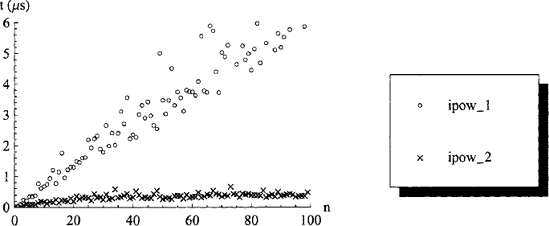
Figure 3.3. Measured performance of the ipow_l and ipow_2 functions which have asymptotic algorithmic complexities of
The actual performance of these two versions of the ipow function can be measured (see Figure 3.3). As expected from the algorithmic complexity, we find that the ipow_2 function is considerably faster for large n .
Figure 3.4. Arrays are the simplest data structure, allowing fast, random access (reading or writing) to the ith element ∀ i |ϵ {0 ... n — 1} where n is the number of elements in the array. Elements cannot be added or removed without copying the whole array.
Asymptotic algorithmic complexity, as we have just described, should be consid-ered first when trying to choose an efficient algorithm or data structure. On the basis of this, we shall now examine some of the wide variety of data structures accessible from F# in the context of the algorithmic complexities of operations over them.
Of all the data structures, arrays will be the most familiar to the scientific programmer. Arrays have the following properties in F#:
Mutable.
Fixed size.
Fast random access and length.
Slow insertion, deletion, concatenation, partition and search.
More specifically, arrays are containers which allow the ith element to be extracted in 0 (1) time (illustrated in figure 3.4). This makes them ideally suited in situations which require a container with fast random access. As the elements of arrays are typically stored contiguously in memory, they are often the most efficient container for iterating over the elements in order. This is the principal alluring feature which leads to their (over!) use in numerically intensive programs. However, many other data structures have asymptotically better performance on important operations.
As we have already seen, the F# language provides a notation for describing arrays:
> let a = [|l; 2|]
  let b = [|3; 4; 5|]
  let C = [|6; 7; 9 |];;
val a : int array
val b : int array
val c : int array
In F#, arrays are mutable, meaning that the elements in an array can be altered in-place.
The element at index i of an array b may be read using the short-hand syntax b. [i]:
> b. [1];;
val it : int = 4
Note that array indices run from {0... n — 1} for an array containing n elements. Array elements may be set using the syntax used for mutable record fields, namely:
> c. [2] <- 8;;
val it : unit = ()
The contents of the array c have now been altered:
> c;;
val it : int array = [|6; 7; 8|]
Any attempt to access an array element which is outside the bounds of the array results in an exception being raised at run-time:
> C. [3] <- 8;;
System.IndexOutOfRangeException: Index was outside the
bounds of the array
The mutability of arrays typically leads to the use of an imperative style when arrays are being used.
The core F# library provides several functions which act upon arrays in the Array module. We shall examine some of these functions before looking at the more exotic array functions offered by F#.
The append function concatenates two arrays:
> Array.append a b;;
val it : int array = [|l; 2; 3; 4; 5|]
The append function has complexity
The concat function concatenates a list of arrays:
> let e = Array.concat [a; b; c];;
val e : int array

> e;;
val it : int array = [|1; 2; 3; 4; 5; 6; 7; 8|]
The concat function has complexity
As we discussed in section 1.6.1, values are referenced so a new variable created from an existing array refers to the existing array. Thus the complexity of creating a new variable which refers to an existing array is
> let d = c;;
val d : int array = [|6; 7; 8|]
The effect of altering the array via either c or d can be seen from both c and d, i.e. they are the same array:
> d.[0] <- 17;;
val it : unit = ()

> c, d;;
val it : int array * int array =
  ([|17; 7; 8|], [|l7; 7; 8|])

> C. [0] <- 6;;
val it : unit = ()

> C, d;;
val it : int array * int array =
  ([| 6; 7; 8 |] , [| 6; 7; 8 |])
The copy function returns a new array which contains the same elements as the given array. For example, the following creates a variable d (superseding the previous d) which is a copy of c:
> let d = Array.copy c;;
val d : int array
Altering the elements of the copied array d does not alter the elements of the original array c:
> d.[0] <- 17;;
val it : unit = ()

> c, d;;
val it : int array * int array =
  ([|6; 7; 8|] , [| 17; 7; 8|])
Aliasing can sometimes be productively exploited in heavily imperative code. However, aliasing is often a source of problems because the sharing of mutable data structures quickly gets confusing. This is why F# encourages a purely functional style of programming using only immutable but performance sometimes leads to the use of mutable data structures because they are more difficult to use correctly but are often faster, particularly for single-threaded use.
The sub function returns a new array which contains a copy of the range of elements specified by a starting index and a length. For example, the following copies a sub-array of 5 elements starting at index 2 (the third element):
> Array.sub e 2 5;;
val it : int array = [|3; 4; 5; 6; 7|]
In addition to these conventional array functions, F# offers some more exotic functions. We shall now examine these functions in more detail.
The higher-orderinit function creates an array, filling the elements with the result of applying the given function to the index i ϵ {0... n — 1} of each element (illustrated in figure 3.5). For example, the following creates the array ai = i2 for i ϵ{0...3}:
> let a = Array.init 4 (fun i -> i * i);;
val a : int array

> a;;
val it : int array = [|0; 1; 4; 9|]
Several higher-order functions are provided to allow functions to be applied to the elements of arrays in various patterns.
The higher-order function iter executes a given function on each element in the given array in turn and returns the value of type unit. The purpose of the function passed to this higher-order function must, therefore, lie in any side-effects it incurs. Hence, the iter function is only of use in the context of imperative, and not functional, programming. For example, the following prints the elements of an int array:
> Array.iter (printf "%d
") a;;
0
1
4
9

Figure 3.6. The higher-order Array. map function creates an array containing the result of applying the given function f to each element in the given array a.
Functions like iter are sometimes referred to as aggregate operators. Several such functions are often applied in sequence, in which case the pipe operator | > can be used to improve clarity. For example, the above could be written equivalently as:
> a |> Array.iter (printf "%d
");;
0
1
4
9
The iter function is probably the simplest of the higher-order functions.
The map function applies a given function to each element in the given array, returning an array containing each result (illustrated in figure 3.6). For example, the following creates the array bi; = a2i:
> let b = Array.map (fun e -> e * e) a;;
val b : int array

> b;;
val b : int array = [|0; 1; 16; 8|]
Higher-order map functions transform data structures into other data structures of the same kind. Higher-order functions can also be used to compute other values from data structures, such as computing a scalar from an array.
The higher-order fold_left and fold_right functions accumulate the result of applying their function arguments to each element in turn. The fold_left function is illustrated in figure 3.7.
In the simplest case, the fold functions can be used to accumulate the sum or product of the elements of an array by folding the addition or multiplication operators over the elements of the array respectively, starting with a suitable base case. For example, the sum of 3, 4, and 5 can be calculated using:
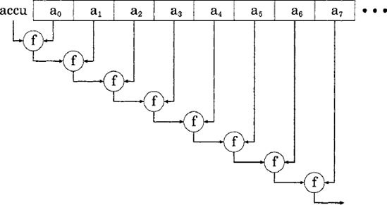
Figure 3.7. The higher-order Array. fold_left function repeatedly applies the given function f to the current accumulator and the current array element to produce a new accumulator to be applied with the next array element.
> Array.fold_left (+) 0 [|3; 4; 5|];;
val it : int = 98
We have already encountered this functionality in the context of the fold_range function developed in section 2.1. However, arrays may contain arbitrary data of arbitrary types (polymorphism) whereas the fold_range function was only applicable to sequences of consecutive ints.
For example, an array could be converted to a list by prepending elements using the cons operator:
> let to_list a =
    Array.fold_right (fun h t -> h :: t) a [];;
val to_list : 'a array -> 'a list
Applying this function to an example array produces a list with the elements of the array:
> to_list [|0; 1; 4; 9|];;
val it : int list = [0; 1; 4; 9]
This to_list function uses fold_right to cumulatively prepend to the list t each element h of the array a in reverse order, starting with the base-case of an empty list []. The result is a list containing the elements of the array. The to_list function is, in fact, already in the Array module:
> Array.to_list [|0; 1; 4; 9 |];;
val it : int list = [0; 1; 4; 9]
Although slightly more complicated than iter and map, the fold_left and fold_right functions are very useful because they can produce results of any type, including accumulated primitive types as well as different data structures.
The contents of an array may be sorted in-place using the higher-order Array. sort function, into an order specified by a given total order function (the predefined compare function, in this case):
> let a = [|l; 5; 3; 4; 7; 9 |];;
val a : int array

> Array.sort compare a;;
val it : unit = ()

> a;;
val it : int array = [|1; 3; 4; 5; 7; 9|]
In addition to these higher-order functions, arrays can be used in pattern matches.
When pattern matching, the contents of arrays can be used in patterns. For example, the vector cross product a x b could be written:
> let cross (a : float array) b =
    match a, b with
    | [|xl; yl; zl|], [|x2; y2; z2|] ->
        [|yl * z2 - zl * y2;
          Zl * X2 - Xl * Z2;
          xl * y2 - yl * x2|]
    | _ -> invalid_arg "cross";;
val cross : float array -> float array -> float array
Note the use of a type annotation on the first argument to ensure that the function applies to float elements rather than the default int elements.
Thus, patterns over arrays can be used to test the number and value of all elements, forming a useful complement to the map and fold algorithms.
Lists have the following properties:
Fast prepend and decapitation (see figure 3.8).
Slow random access, length, insertion, deletion, concatenation, partition and search.
Arguably the simplest and most commonly used data structure, lists allow two fundamental operations. The first is decapitation of a list into two parts, the head (the first element of the list) and the tail (a list containing the remaining elements). The second is the reverse operation of prepending an element onto a list to create a new list. The complexities of both operations are
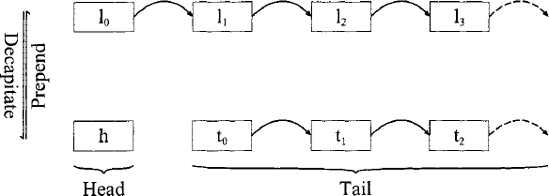
Figure 3.8. Lists are the simplest, arbitrarily-extensible data structure. Decapitation splits a list li iϵ{0... n — 1} into the head element h and the tail list ti i ϵ{0 ... n — 2}.
As we have already seen, the F# language implements lists natively. In particular, the cons operator : : can be used both to prepend an element and to represent decapitated lists in patterns. Unlike arrays, the implementation of lists is functional, so operations on lists produce new lists.
The List module contains the iter, map, fold_left and fold_right functions, equivalent to those for arrays, a flatten function, which provides equivalent functionality to that of Array. concat (i.e. to concatenate a list of lists into a single list). In particular, the append function has the pseudonym @:
> [1; 2] @ [3; 4];;
val it : int list = [1; 2; 3; 4]
The List module also contains several functions for sorting and searching.
The contents of a list may be sorted using the higher-order List. sort function, into an order specified by a given total order function (the predefined compare function, in this case):
> List.sort compare [1; 5; 3; 4; 7; 9];;
val it : int list = [1; 3; 4; 5; 7; 9]
Lists can be searched using a variety of functions.
There are three main forms of searching provided by the List module.
An element may be tested for membership in a list using the List. mem function:
> List.mem 4 [1; 3; 4; 5; 7; 9];;
val it : bool = true

> List.mem 6 [1; 3; 4; 5; 7; 9];;
val it : bool = false
This is the simplest form of searching that can be applied to lists and is an easy but inefficient way to handle sets of values.
The first element in a list that matches a given predicate function may be extracted using the higher-order List. find function:
> List.find (fun i -> (i-6)*i > 0) [1; 3; 4; 5; 7; 9];;
val it : int = 7
This function raises an exception if all the elements in the given list fail to match the given predicate:
> List.find (fun i -> (i-6)*i = 0) [1; 3; 4; 5; 7; 9];;
System.IndexOutOfRangeException: Index was outside the
bounds of the array
The related function List. find_al1 returns the list of all elements that match the given predicate function:
> [1; 3; 4; 5; 7; 9]
  |> List.find_all (fun i -> (i-6)*i > 0);;
val it : int list = [7; 9]
Searching lists using predicate functions works well when several different predicates are used and performance is unimportant.
The contents of a list of key-value pairs may be searched using the List. assoc function to find the value corresponding to the first matching key. For example, the following list list contains (i, i2) key-value pairs:
> let list =
    [for i in 1 .. 5 ->
       i, i*i 1;;
val list : (int * int) list

> list;;
val it : (int * int) list
  = f(l, 1); (2, 4); (3, 9); (4, 16); (5, 25)]
Searching list for the key i = 4 using the List. assoc function finds the corresponding value i2 = 16:
> List.assoc 4 list;;
val it : int = 16
As we have seen, lists are easily searched in a variety of different ways. Consequently, lists are one of the most useful generic containers provided by the F# language. However, testing for membership is really a set-theoretic operation and the built-in HashSet and Set modules provide asymptotically more efficient ways to implement sets as well as extra functionality. Similarly, the ability to map keys to values in an association list is provided more efficiently by hash tables and maps. All of these data structures are discussed later in this chapter.
The ability to grow lists makes them ideal for filtering operations based upon arbitrary predicate functions. The List .partition function splits a given list into two lists containing those elements which match the predicate and those which do not. The following example uses the predicate xi ≤ 3:
> List.partition (fun x -> x <= 3) [1 .. 5];;
val it : int list * int list = ([1; 2; 3], [4; 5])
Similarly, the List.filter function returns a list containing only those elements which matched the predicate, i.e. the first list that List. partition would have returned:
> List.filter (fun x -> x <= 3) [1 .. 5];;
val it : int list = [1; 2; 3]
The partition and filter functions are ideally suited to arbitrarily extensible data structures such as lists because the length of the output(s) cannot be precalculated.
In addition to the conventional higher-order iter, map, folds, sorting and searching functions, the List module contains several functions which act upon pairs of lists. These functions all assume the lists to be of equal length. If they are found to be of different lengths then an Invalid_argument exception is raised. We shall now elucidate these functions using examples from vector algebra.
The higher-order function map2 applies a given function to each pair of elements from two equal-length lists, producing a single list containing the results. The type of the map2 function is:
val map2 :
  ('a -> 'b -> 'c) -> 'a list -> 'b list -> 'c list
The map2 function can be used to write a function to convert a pair of lists into a list of pairs:
> let list_combine a b =
    List.map2 (fun a b -> a, b) a b;;
val list_combine : 'a list -> 'b list -> ('a, 'b) listApplying the 1is t_combine function to apair of lists of equal lengths combines them into a list of pairs:
> list_combine [1; 2; 3] ["a"; "b"; "c"];;
val it : (int * string) list =
  [(1, "a"); (2, "b"); (3, "c")]
Applying the list_combine function to a pair of lists of unequal lengths causes an exception to be raised by the map2 function:
> list_combine [1; 2; 3] [2; 3; 4; 5];;
Microsoft.FSharp.InvalidArgumentException: map2
In fact, the functionality of this list_combine function is already provided by the combine function in the List module of the F# standard library.
Vector addition for vectors represented by lists can be written in terms of the map2 function:
> let vec_add (a : float list) b =
    List.map2 (+) a b;;
val vec_add : float list -> float list -> float list
When given a pair of lists a and b of floating-point numbers, this function creates a list containing the sum of each corresponding pair of elements from the two given lists, i.e. a + b:
> vec_add [1.0; 2.0; 3.0] [2.0; 3.0; 4.0];;
val it : float list = [3.0; 5.0; 7.0]
The higher-order fold_left2 and fold_right2 functions in the List module are similar to the fold_left and fold_right functions, except than they act upon two lists simultaneously instead of one. The types of these functions are:
val fold_left2 :
  ('a -> 'b -> 'c -> 'a) -> 'a -> 'b list -> 'c list ->
    'a
val fold_right2 :
  ('a -> 'b -> 'c -> 'c) -> 'a list -> 'b list -> 'c ->
    'c
Thus, the fold_left2 and fold_right2 functions can be used to implement many algorithms which consider each pair of elements in a pair of lists in turn. For example, the vector dot product could be written succinctly using fold_left2 by accumulating the products of element pairs from the two lists:
> let vec_dot (a : float list) (b : float list) =
    List.fold_left2 (fun dab->d+a*b) O.Oab;;
val vec_dot : float list -> float list -> float
When given two lists, a and b, of floating-point numbers, this function accumulates the products a,i × bi of each pair of elements from the two given lists, i.e. the vector dot product a • b:
> vec_dot [1.0; 2.0; 3.0] [2.0; 3.0; 4.0];;
val it : float =20.0
The ability to write such functions using maps and folds is clearly an advantage in the context of scientific computing. Moreover, this style of programming can be seamlessly converted to using much more exotic data structures, as we shall see later in this chapter. In some cases, algorithms over lists cannot be expressed easily in terms of maps and folds. In such cases, pattern matching can be used instead.
Patterns over lists can not only reflect the number and value of all elements, as they can in arrays, but can also be used to test initial elements in the list using the cons operator : : to decapitate the list. In particular, pattern matching can be used to examine sequences of list elements. For example, the following function "downsamples" a signal, represented as a list of floating-point numbers, by averaging pairs of elements:
> let rec downsample : float list -> float list =
    function | [] -> []
    | hl::h2::t -> 0.5 * (h1 + h2) :: downsample t
    | [_] -> invalid_arg "downsample";;
val downsample : float list -> float list
This is a simple, recursive function which uses a pattern match containing three patterns. The first pattern downsamples the empty list to the empty list. This pattern acts as the base-case for the recursive calls of the function (equivalent to the base-case of a recurrence relation). The second pattern matches the first two elements in the list (hi and h2) and the remainder of the list (t). Matching this pattern results in prepending the average of h1 and h2 onto the list resulting from downsampling the remaining list t. The third pattern matches a list containing any single element, raising an exception if this erroneous input is encountered:
> downsample [5.0];;
Exception: Invalid_argument "downsample".
As these three patterns are completely distinct (any input list necessarily matches one and only one pattern) they could, equivalently, have been presented in any order in the pattern match.
The downsample function can be used to downsample an eight-element list into a four-element list by averaging pairs of elements:
> [0.0; 1.0; 0.0; −1.0; 0.0; 1.0; 0.0; −1.0]
  |> downsample;;
val it : float list = [0.5; −0.5; 0.5; −0.5]
The ability to perform pattern matches over lists is extremely useful, resulting in a very concise syntax for many operations which act upon lists.
Note that, in the context of lists, the iter and map higher-order functions can be expressed succinctly in terms of folds:
let iter f list =
  List.fold_left (fun () e -> f e) () list
let map f list =
  List.fold_right (fun h t -> f h :: t) list []
and that all of these functions can be expressed, albeit more verbosely, using pattern matching. The iter function simply applies the given function f to the head h of the list and then recurses to iterate over the element in the tail t:
let rec iter f = function
  | [] -> ()
  | h::t -> f h; iter f t
The map function applies the given function f to the head h of the list, prepending the result f h onto the result map f t of recursively mapping over the elements in the tail t:
let rec map f = function
  | [] -> []
  | h: : t - > f h : : map f t
The fold_left function applies the given function f to the current accumulator accu and the head h of the list, passing the result as the accumulator for folding over the remaining elements in the tail t of the list:
let rec fold_left f accu list =
  match list with
  | h::t -> fold_left f (f accu h) t
  | [] -> accu
The fold_right function applies the given function f to the head h of the list and the result of recursively folding over the remaining elements in the tail t of the
list:
let rec fold_right f list accu =
  match list with
  | h::t -> f h (fold_right f t accu)
  | [] -> accu
Thus, the map and fold functions can be thought of as higher-order functions which have been factored out of many algorithms. In the context of scientific programming, factoring out higher-order functions can greatly increase clarity, often providing new insights into the algorithms themselves. In chapter 6, we shall pursue this, developing several functions which supplement those in the standard library.
Having examined the two simplest containers provided by the F# language itself, we shall now examine some more sophisticated containers which are provided in the standard library.
Sets have the following properties:
In the context of data structures, the term "set" typically means a sorted, unique, associative container. Sets are "sorted" containers because the elements in a set are stored in order according to a given comparison function. Sets are "unique" containers because they do not duplicate elements (adding an existing element to a set results in the same set). Sets are "associative" containers because elements determine how they are stored (using the specified comparison function).
The F# standard library provides sets which are implemented as balanced binary trees[11]. This allows a single element to be added or removed from a set containing n elements in O (ln n) time. Moreover, the F# implementation also provides functions union, inter and diff for performing the set-theoretic operations union, intersection and difference efficienctly.
In order to implement the set-theoretic operations between sets correctly, the sets used must be based upon the same comparison function. If no comparison function is specified then the built-in compare function is used by default. Sets implemented using custom comparison functions can be created using the Set. Make function.
The empty set can be obtained as:
> Set.empty;;
val it : Set<'a>
The type Set< ' a> represents a set of values of type ' a.
A set containing a single element is called a singleton set and can be created using the Set.singleton function:
> let setl = Set.singleton 3;;
val setl : Set<int>
Sets can also be created from sequences using the set function:
> set [1; 2; 3];;
val it : Set<int> = seq [1; 2; 3]
Once created, sets can have elements added and removed.
As sets are implemented in a functional style, adding an element to a set returns a new set that shares immutable data with the old set:
> let set2 = Set.add 5 setl;;
val set2 : Set<int>
Both the old set and the new set are still valid:
> set1, set2;;
val it : Set<int> * Set<int> = (seq [3], seq [3; 5])
Sets remove duplicates:
> let S = set [10; 1; 9; 2; 8; 4; 7; 4; 6; 7; 7];;
val s : Set<int>
A set may be converted into other data structures, such as a list using the to_list function in the Set module:
> Set.to_list s;;
val it : int list = [1; 2; 4; 6; 7; 8; 9; 10]
As we shall see in section 3.8, sets are also a kind of sequence.
The number of elements in a set, known as the cardinality of the set, is given by:
> Set. cardinal s;;
val it : int = 8
Perhaps the most obvious functionality of sets is that of set-theoretic operations.
We can also demonstrate the set-theoretic union, intersection and difference operations. For example:
{1, 3,5} U {3, 5, 7} = {1,3,5, 7}> Set.union (set [1; 3; 5]) (set [3; 5; 7]);;
val it : Set<int> = [1; 3; 5; 7]
{1,3,5} ? {3,5, 7}={3,5}
> Set.inter (set [1; 3; 5]) (set [3; 5; 7]);;
val it : Set<int> = [3; 5]
{1,3,5}{3,5,7} = {1}
> Set.diff (set [1; 3; 5]) (set [3; 5; 7]);;
val it : Set<int> = [1]Set union and difference can also be obtained by applying the + and - operators:
> set [1; 3; 5] + set [3; 5; 7];;
val it : Set<int> = [1; 3; 5; 7]

> set [1; 3; 5] - Set [3; 5; 7];;
val it : Set<int> = [1]
The subset function tests if A ⊂ B. For example, {4,5,6} ⊂ {1... 10}:
> Set.subset (set [2; 4; 6]) s;;
val it : bool = true
Of the data structures examined so far (lists, arrays and sets), only sets are not concrete data structures. Specifically, the underlying representation of sets as balanced binary trees is completely abstracted away from the user. In some languages, this can cause problems with notions such as equality but, in F#, sets can be compared safely using the built-in comparison operators and function.
Although sets are non-trivial data structures internally, the polymorphic comparison functions (<, <=, =, >=, >, <> and compare) can be applied to sets and data structures containing sets in F#:
> Set.of_list [1; 2; 3; 4; 5] =
    Set.of_list [5; 4; 3; 2; 1];;
val it : bool = true
In chapter 12, we shall use a set data structure to compute the set of nth-nearest neighbours in a graph and apply this to atomic-neighbour computations on a simulated molecule. In the meantime, we have more data structures to discover.
Hash tables have the following properties:
A hash table is an associative container mapping keys to corresponding values. We shall refer to the key-value pairs stored in a hash table as bindings or elements.
In terms of utility, hash tables are an efficient way to implement a mapping from one kind of value to another. For example, to map strings onto functions. In order to provide their functionality, hash tables provide add, replace and remove functions to insert, replace and delete bindings, respectively, a find function to return the first value corresponding to a given key and a find_all function to return all corresponding values.
Internally, hash tables compute an integer value, known as a hash, from each given key. This hash of a key is used as an index into an array in order to find the value corresponding to the key. The hash is computed from the key such that two identical keys share the same hash and two different keys are likely (but not guaranteed) to produce different hashes. Moreover, hash computation is restricted to
The F# standard library contains an imperative implementation of hash tables in the Hashtbl module.
The Hashtbl. of_seq function can be used to create hash tables from association sequences:
> let m =
    ["Hydrogen", 1.0079; "Carbon", 12.011;
     "Nitrogen", 14.00674; "Oxygen", 15.9994;
     "Sulphur", 32.06]
    |> Hashtbl.of_seq;;
val m : Hashtbl.HashTable<string, float>
The resulting hash table m, of type Hashtbl .HashTable <string, float,> represents the following mapping from strings to floating-point values:
Hydrogen | → | 1.0079 |
Carbon | → | 12.011 |
Nitrogen | → | 14.00674 |
Oxygen | → | 15.9994 |
Sulphur | → | 32.06 |
Having been filled at run-time, the hash table may be used to look-up the values corresponding to given keys. For example, we can find the average atomic weight of carbon:
> Hashtbl.find m "Carbon";;
val it : float = 12.011
Looking up values in a hash table is such a common operation that a more concise syntax for this operation has been provided via the getter of the Item member, accessed using the notation:
m. [key]
For example:
> m.["Carbon"];;
val it : float = 12.011
Hash tables also allow bindings to be added and removed.
A mapping can be added using the Hashtbl. add function:
> Hashtbl.add m "Tantalum" 180.9;;
val it : unit = ()
Note that adding a new key-value binding shadows any existing bindings rather than replacing them. Subsequently removing such a binding makes the previous binding for the same key visible again if there was one.
Bindings may be replaced using the Hashtbl. replace function:
> Hashtbl.replace m "Tantalum" 180.948;;
val it : unit = ()
Any previous binding with the same key is then replaced.
The setter of the Item property is also implemented, allowing the following syntax to be used to replace a mapping in a hash table m:
m. [key] <- value
If the hash table did not contain the given key then a new key is added. For example, the following inserts a mapping for tantalum:
> m.["Tantalum"] <- 180.948;;
val it : unit = ()
If necessary, we can also delete mappings from the hash table, such as the mapping for Oxygen:
> Hashtbl.remove m "Oxygen";;
val it : unit = ()
The usual higher-order functions are also provided for hash tables.
The remaining mappings in the hash table are most easily printed using the iter function in the Hashtbl module:
> Hashtbl.iter (printf "%s -> %f
") m;;
Carbon -> 12.011
Nitrogen -> 14.00674
Sulphur -> 32.06
Hydrogen -> 1.007 9
Tantalum -> 180.948
Note that the order in which the mappings are supplied by Hashtbl. iter (and map and fold) is effectively random. In fact, the order is related to the hash function.
Hash tables can clearly be useful in the context of scientific programming. However, a functional alternative to these imperative hash tables can sometimes be desirable. We shall now examine a functional data structure which uses different techniques to implement the same functionality of mapping keys to corresponding values.
Maps have the following properties:
We described the functional implementation of the set data structure provided by F# in section 3.4. The core F# library provides a similar data structure known simply as a map[13].
Much like a hash table, the map data structure associates keys with corresponding values. Consequently, the map data structure also provides add and remove functions to insert and delete mappings, respectively, and a find function which returns the value corresponding to a given key.
Unlike hash tables, maps are represented internally by a balanced binary tree, rather than an array, and maps differentiate between keys using a specified total ordering function, rather than a hash function.
Due to their design differences, maps have the following advantages over hash tables:
Immutable: operations on maps derive new maps without invalidating old maps.
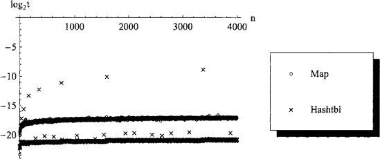
Figure 3.9. Measured performance (time t in seconds) for inserting key-value pairs into hash tables and functional maps containing n — 1 elements. Although the hash table implementation results in better average-case performance, the 0 (n) time-complexity incurred when the hash table is resized internally produces much slower worst-case performance by the hash table.
Stable 0 (log n) time-complexity for inserting and removing a mapping, compared to unstable, amortized Θ(1) time-complexity in the case of hash tables (which may take up to 0(n) for some insertions, as illustrated in figure 3.9).
Maps are based upon comparison and hash tables are based upon hashing. Comparisons are easier to define and more readily available.
If comparison is faster than hashing (e.g. for structurally large keys, where comparison can return early) then a map may be faster than a hash table.
The key-value pairs in a map are kept sorted by key.
However, maps also have the following disadvantages compared to hash tables:
Logarithmic 0 (ln n) time-complexity for insertion, lookup and removal, compared to amortized Θ(1) time-complexity in the case of hash tables (see figure 3.9).
If comparison is slower than hashing (e.g. for small keys) then a hash table is likely to be faster than a map.
In single threaded applications, a map is typically 10 x slower than a hash table in practice.
We shall now demonstrate the functionality of the map data structure reusing the example of mapping strings to floating-point values. A map data structure containing no mappings is represented by the value:
> let m = Map.empty;;
val m : Map<'a, 'b>
Note that this value is polymorphic, allowing the empty map to be used as the basis of mappings between any types.
Mappings may be added to m using the Map. add function. As a functional data structure, adding elements to a map returns a map containing both the new and old mappings. Hence we repeatedly supersede the old data structure m with a new data structure m:
A map may be built from a list using the Map. of_1ist function:
> let m =
    Map.of_list
    ["Hydrogen", 1.0079; "Carbon", 12.011;
     "Nitrogen", 14.00674; "Oxygen", 15.9994;
     "Sulphur", 32.06]
val m : Map<string, float>
Note that the type has been inferred to be a mapping from strings to floats. The contents of a map can be converted to a list using the fold function:
> let list_of map =
    Map.fold (fun h t -> h :: t) map [];;
val list_of : Map<'a, 'b> -> ('a, 'b) list
Once created, a map can be searched.
We can use the map m to find the average atomic weight of carbon:
> Map.find "Carbon" m;;
val it : float = 12.011
The syntax used for hash table lookup can also be used on maps:
> m. ["Carbon"];;
val it : float = 12.011
However, as maps are immutable they cannot be altered in-place and, consequently, the Item setter method is not implemented. Adding a binding to a map produces a new immutable map that shares much of its internals with the old map (which remains valid). For example, we can create a new map with an additional binding:
> let m2 = Map.add "Tantalum" 180.948 m;;
val m2 : Map<string, float>
Both the old map m and the new map m2 are valid:
> list_of m, list_of m2;;
val it : (string * float) list * (string * float) list
= ([("Carbon", 12.011); ("Hydrogen", 1.0079);
    ("Nitrogen", 14.00674); ("Oxygen", 15.9994);
    ("Sulphur", 32.06)] ,
   [("Carbon", 12.011); ("Hydrogen", 1.0079);
    ("Nitrogen", 14.00674); ("Oxygen", 15.9994);
    ("Sulphur", 32.06); ("Tantalum", 180.948)])]
Note that the key-value pairs are sorted by key, alphabetically in this case.
Deleting mappings from the functional map data structure produces a new data structure containing most of the old data structure:
> Map.remove "Oxygen" m2;;
val it : Map<string, float>
  = [("Carbon", 12.011); ("Hydrogen", 1.0079);
     ("Nitrogen", 14.00674); ("Sulphur", 32.06);
     ("Tantalum", 180.948)]
Maps contain the usual higher-order functions.
The remaining mappings are most easily printed by iterating a print function over the key-value pairs:
> Map. iter (printf "%s -> %f
") m2;;
Carbon -> 12.011
Hydrogen -> 1.0 0 79
Nitrogen -> 14.00674
Oxygen -> 15.9 9 94
Sulphur -> 32.06
Tantalum -> 180.948
Note that m2 still contains the entry for oxygen as deleting this binding created a new map that was discarded.
The ability to evolve the contents of data structures along many different lineages during the execution of a program can be very useful. This is much easier when the data structure provides a functional, rather than an imperative, interface. In an imperative style, such approaches would most likely involve the inefficiency of explicitly duplicating the data structure (e.g. using the Hashtbl. copy function) at each fork in its evolution. In contrast, functional data structures provide this functionality naturally and, in particular, will share data between lineages.
Having examined the data structures provided with F#, we shall now summarise the relative advantages and disadvantages of these data structures using the notion of algorithmic complexity developed in section 3.1.
Table 3.2. Functions implementing common operations over data structures.
Array | List | Set | Hash table | Map | |
|---|---|---|---|---|---|
Create |
|
|
|
|
|
Insert | - | - |
|
|
|
Search |
|
|
|
|
|
Remove | - |
|
|
|
|
Sort |
|
| N/A | N/A | N/A |
Index |
|
| N/A |
|
|
As we have seen, the complexity of operations over data structures can be instrumental in choosing the appropriate data structure for a task. Consequently, it is beneficial to compare the asymptotic complexities of common operations over various data structures. Table 3.2 shows several commonly-used functions. Table 3.3 gives the asymptotic complexities of the algorithms used by these functions, for data structures containing n elements.
Arrays are ideal for computations requiring very fast random access. Lists are ideal for accumulating sequences of unknown lengths. The immutable set implementation in the Set module provides very fast set-theoretic operations union, intersection and difference. Hash tables are ideal for random access via keys that are not consecutive integers, e.g. sparsely-distributed keys or non-trivial types like strings.
The F# standard library contains other data structures such as mutable sets based upon hash tables. These do not offer fast set-theoretic operations but testing for membership is likely to be several times faster with mutable rather than immutable sets.
Having examined the various containers built-in to F#, we shall now examine a generalisation of these containers which is easily handled in F#.
The .NET collection called IEnumerable is known as Seq in F#. This collection provides an abstract representation of any lazily evaluated sequences of values. A lazily evaluated sequence only evaluates the elements when they are required, i.e. the sequence does not need to be stored explicitly.
The list, array, set, map and hash table containers all implement the Seq interface and, consequently, can be used as abstract sequences.
For example, the following function doubles each value in a sequence:
> let double s =
    Seq.map ((*) 2) s;;
val double : #seq<int> -> seq<int>
Note that the argument to the double function is inferred to have the type #seq<int>, denoting objects of any class that implements the Seq interface, but the result of double is of the type seq<int>.
For example, this double function can be applied to arrays and sets:
> double [|1; 2; 3 I];;
val it : seq<int> = [2; 4; 6]

> double (set [1; 2; 3]);;
val it : seq<int> = [2; 4; 6]
Sequences can be generated from functions using the Seq. generate function. In particular, such sequences can be infinitely long. The generate function accepts three functions as arguments. The first argument opens the stream. The second argument generates an option value for each element with None denoting the end of the stream. The third argument closes the stream.
This abstraction has various uses:
Functions that act sequentially over data structures can be written more uniformly in terms of Seq. For example, by using
Seq. foldinstead ofList.fold_left or Array.fold_left.Simplifies code interfacing different types of container.
The higher-order
Seq. mapandSeq. filterfunctions are lazy, so a series of maps and filters is more space efficient and is likely to be faster using sequences rather than lists or arrays.
Sequences are useful in many situations but their main benefit is simplicity.
The array, list, set, hash table and map containers are all homogeneous containers, i.e. for any such container, the elements must all be of the same type. Containers of elements which may be of one of several different types can also be useful. These are known as heterogeneous containers.
Heterogeneous containers can be denned in F# by first creating a variant type which combines the types allowed in the container. For example, values of this variant type number may contain data representing elements from the sets Z, R or C:
> type number =
    | Integer of int
    | Real of float
    | Complex of float * float;;
A homogeneous container over this unified type may then be used to implement a heterogeneous container. The elements of a container of type number list can contain Integer, Real or Complex values:
> let nums = [Integer 1; Real 2.0; Complex (3.0, 4.0)];;
val nums : number list
Let us consider a simple function to act upon the effectively heterogeneous container type number list. A function to convert values of type number to the built-in type Math. Complex may be written:
> let complex_of_number = function
  | Integer n -> complex (float n) 0.0
  | Real x -> complex x 0.0
  | Complex(x, y) -> complex x y;;
val complex_of_number : number -> Math.Complex
For example, mapping the complex_of_number function over the number list called nums gives a Complex. t list:
ist.map complex_of_number
val it : Complex.t list =
  [l.Or + 0.0i; 2.Or + O.Oi; 3.Or + 4.0i]
The list, set, hash table and map data structures can clearly be useful in a scientific context, in addition to conventional arrays and the heterogeneous counterparts of these data structures. However, a major advantage of F# lies in its ability to create and manipulate new, custom-made data structures. We shall now examine this aspect of scientific programming in F#.
In addition to the built-in data structures, the ease with which the F# language allows tuples, records and variant types to be handled makes it an ideal language for creating and using new data structures. Trees are the most common such data structure.
A tree is a self-similar data structure used to store data hierarchically. The origin of a tree is, therefore, itself a tree, known as the root node. As a self-similar, or recursive, data structure, every node in a tree may contain further trees. A root that contains no further trees marks the end of a lineage in the tree and is known as a leaf node.
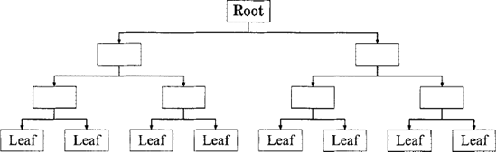
Figure 3.10. A perfectly-balanced binary tree of depth x = 3 containing 2X+1 — 1 = 15 nodes, including the root node and 2X = 8 leaf nodes.
The simplest form of tree is a recursive data structure containing an arbitrarily-long list of trees. This is known as an n-ary tree and may be represented in F# by the type:
> type tree = Node of tree list;;
A perfectly balanced binary tree of depth d is represented by an empty node for d = 0 and a node containing two balanced binary trees, each of depth d — 1, for d > 0. This simple recurrence relation is most easily implemented as a purely functional, recursive function:
> let rec balanced_tree = function
  | 0 -> Node []
  | n ->
      Node [balanced_tree(n-1); balanced_tree(n-1)];;
val balanced_tree : int -> tree
The tree depicted in figure 3.10 may then be constructed using:
> let example = balanced_tree 3;;
val example : tree =
  Node
   [Node [Node [Node []; Node []];
          Node [Node []; Node []]];
    Node [Node [Node []; Node []];
          Node [Node []; Node []]]]
We shall use this example tree to demonstrate more sophisticated computations over trees.
Functions over the type tree are easily written. For example, the following function counts the number of leaf nodes:
> let rec leaf_count = function
| Node [] -> 1
    | Node list ->
        Seq.fold (fun s t -> s + leaf_count t) 0 list;;
val leaf_count : tree -> int

> leaf_count example;;
val it : int = 8
Trees represented by the type tree are of limited utility as they cannot contain additional data in their nodes. An equivalent tree which allows arbitrary, polymorphic data to be placed in each node may be represented by the type:
> type 'a ptree = PNode of 'a * 'a ptree list;;
As a trivial example, the following function traverses a value of type tree to create an equivalent value of type ptree which contains a zero in each node:
> let rec zero_ptree_of_tree (Node list) =
    PNode(0, List.map zero_ptree_of_tree list);;
val zero_ptree_of_tree : tree -> int ptree
For example:
> zero_ptree_of_tree (Node [Node []; Node [];;
val it : int ptree =
  PNode (0, [PNode (0, []); PNode (0, [])])
As a slightly more interesting example, consider a function to convert a value of type tree to a value of type ptree, storing unique integers in each node of the resulting tree.
We begin by denning a higher-order function auxl that accepts a function f that will convert a tree into a ptree and uses this to convert the head of a list h and prepend it onto a tail list t in an accumulator that also contains the current integer n (i.e. the accumulator will be of type int * int ptree list):
> let auxl f h (n, t) =
    let n, h = f h n
    n, h : : t;;
val auxl :
  ('a -> 'b -> 'c * 'd) -> 'a -> 'b * 'd list ->
    'c * 'd list
A function aux2 to convert a tree into a ptree can be written by folding the aux1 function over the counter n and child trees 1ist, accumulating a new counter n' and a list plist of child trees.
> let rec aux2 (Node list) n =
    let n', plist =
      List.fold__right (auxl aux2) list (n +1, [])
    n', PNode(n, plist);;
val aux2 : tree -> int -> int * int ptree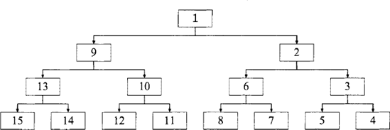
Figure 3.11. The result of inserting an integer counter into each node of the tree depicted in figure 3.10 using the counted_ptree_of_tree function.
For example:
> aux2 (Node [Node []; Node []; Node []]) 1;;
val it : int * int ptree =
  (5, PNode (1, [PNode (4, []);
                 PNode (3, []);
                 PNode (2, [])]))
The aux2 function can be used to convert a tree into a ptree with counted nodes by supplying an initial counter of 1 and stripping off the final value of the counter from the return value of aux2 using the built-in function snd to extract the second part of a 2-tuple:
> let rec counted_ptree_of_tree tree =
    snd (aux2 tree 1);;
val counted_ptree_of_tree : tree -> int ptree
Applying this function to our example tree produces a more interesting result (illustrated in figure 3.11):
> counted_ptree_of_tree example;;
val it : int ptree =
  PNode (1,
   [PNode (9, [PNode (13, [PNode (15, []);
                           PNode (14, [])]);
               PNode (10, [PNode (12, []);
                           PNode (11, [])])]);
   PNode (2,  [PNode (6, [PNode (8, []);
                         PNode (7, [])]);
               PNode (3, [PNode (5, []);
                         PNode (4, [])])])])
Note that the use of a right fold in the aux2 function allowed the child trees to be accumulated into a list in the same order that they were given but resulted in numbering from right to left.
In practice, storing the maximum depth remaining in each branch of a tree can be useful when writing functions to handle trees. Values of our generic tree type may be converted into the ptree type, storing the integer depth in each node, using the following function:
> let rec depth_ptree_of_tree (Node list) =
    let list = List.map depth_ptree_of_tree list
    let depth_of (PNode(d, _)) = d
    let depth = Seq.fold (+) (-1) (Seq.map depth_of list)
    PNode(depth + 1, list);;
val depth_ptree_of_tree : tree -> int ptree
This function first maps itself over the child trees to get their depths. Then it folds an anonymous function that computes the maximum of each depth (note the use of partial application of max) with an accumulator that is initially —1. Finally, a node of a ptree is constructed from the depth and the converted children.
Applying this function to our example tree produces a rather uninteresting, symmetric set of branch depths:
> depth_ptree_of_tree example;;
val it : int ptree =
  PNode (3,
   [PNode (2,
     [PNode (1, [PNode (0, []); PNode (0, [])]);
      PNode (1, [PNode (0, []) , PNode (0, [])])]);
    PNode (2,
     [PNode (1, [PNode (0, []); PNode (0, [])]);
      PNode (1, [PNode (0, []); PNode (0, [])])])])
Using a tree of varying depth provides a more interesting result. The following function creates an unbalanced binary tree, effectively representing a list of increasingly-deep balanced binary trees in the left children:
> let rec unbalanced_tree n =
    let aux n t = Node [balanced_tree n; t]
    List.fold_right aux [0 .. n - 1] (Node []);;
val unbalanced_tree : int -> tree
This can be used to create a wonky tree:
> let wonky = unbalanced_tree 3;;
val wonky : tree =
  Node
   [Node [];
    Node
     [Node [Node []; Node []];;
      Node [Node [Node [Node []; Node []];
                  Node [Node []; Node []]];
            Node []]]]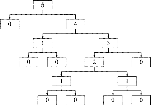
Converting this wonky tree into a tree containing the remaining depth in each node we obtain a more interested result (illustrated in figure 3.12):
> depth_ptree_of_tree wonky;;
val it : int ptree =
  PNode (5,
   [PNode (0, []);
    PNode (4,
     [.PNode (1, [PNode (0, []); PNode (0, [])]);
       PNode (3,
       [PNode (2,
         [PNode (1, [PNode (0, []); PNode (0, [])]);
          PNode (1, [PNode (0, []); PNode (0, [])])]);
        PNode (0, [])])])])
However, the ability to express a tree in which each node may have an arbitrary number of branches often turns out to be a hindrance rather than a benefit. Consequently, the number of branches allowed at each node in a tree is often restricted to one of two values:
zero branches for leaf nodes and
a constant number of branches for all other nodes.
Trees which allow only zero or two branches, known as binary trees, are particularly prolific as they form the simplest class of such trees[14], simplifying the derivations of the complexities of operations over this kind of tree.
Although binary trees could be represented using the tree or ptree data structures, this would require the programmer to ensure that all functions acting upon these types produced node lists containing either zero or two elements. In practice, this is likely to become a considerable source of human error and, therefore, of programmer frustration. Fortunately, when writing in F#, the type system can be used to enforce the use of a valid number of branches at each node. Such automated checking not only removes the need for careful inspection by the programmer but also removes the need to perform run-time checks of the data, improving performance. A binary tree analogous to our tree data structure can be defined as:
> type bin_tree =
    | Leaf
    | Node of bin_tree * bin_tree;;
A binary tree analogous to our ptree data structure can be defined as:
> type 'a pbin_tree =
    | Leaf of 'a
    | Node of 'a pbin_tree * 'a * 'a pbin_tree;;
Values of type ptree which represent binary trees may be converted to this pbin_tree type using the following function:
> let rec pbin_tree_of_ptree = function
    | PNode(v, []) -> Leaf v
    | PNode(v, [1; r]) ->
        Node(pbin_tree_of_ptree 1,
             v,
             pbin_tree_of_ptree r)
    | _ -> invalid_arg "pbin_tree_of_ptree";;
val pbin_tree_of_jptree : 'a ptree -> 'a pbin_tree
For example, the arbitrary-branching-factor example tree may be converted into a binary tree using the pbin_tree_of _ptree function:
> pbin_tree_of_ptree (depth_ptree_of_tree example);;
val it : int pbin_tree =
  Node
   (Node
     (Node (Leaf 0, 1, Leaf 0),
      2,
      Node (Leaf 0, 1, Leaf 0)),
    3,
    Node
     (Node (Leaf 0, 1, Leaf 0),
      2,
      Node (Leaf 0, 1, Leaf 0)))
Note that the ' a pbin_tree type, which allows arbitrary data of type ' a to be stored in all nodes, could be usefully altered to an (' a, ' b) t type which allows
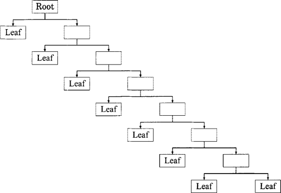
Figure 3.13. A maximally-unbalanced binary tree of depth x = 7 containing 2x + 1 = 15 nodes, including the root node and x + 1 = 8 leaf nodes.
arbitrary data of type 'a to be stored in leaf nodes and arbitrary data of type 'b to be stored in all other nodes:
> type ('a, 'b) t =
    | Leaf of 'a
    | Node of 'b * ('a, 'b) t * ('a, 'b) t;;
Having examined the fundamentals of tree-based data structures, we shall now examine the two main categories of trees: balanced trees and unbalanced trees.
Balanced trees, in particular balanced binary trees, are prolific in computer science literature. As the simplest form of tree, binary trees simplify the derivation of algorithmic complexities. These complexities often depend upon the depth of the tree. Consequently, in the quest for efficient algorithms, data structures designed to maintain approximately uniform depth, known as balanced trees, are used as the foundation for a wide variety of algorithms.
A balanced tree (as illustrated in figure 3.10) can be denned as a tree for which the difference between the minimum and maximum depths tends to a finite value for any such tree containing n nodes in the limit[15] n → ∞. Practically, this condition is often further constricted to be that the difference between the minimum and maximum depths is no more than a small constant.
The efficiency of balanced trees stems from their structure. In terms of the number of nodes traversed, any node in a tree containing either n nodes or n leaf nodes may be reached by 0 (log n) traversals from the root.
For example, the set and map data structures provided in the F# standard library both make use of balanced binary trees internally. This allows them to provide single-element insertion, removal and searching in O (ln n) time-complexity.
For detailed descriptions of balanced tree implementation, we refer the eager reader to the relevant computer science literature [3] and, in particular, to an article in The F#.NET Journal [12]. However, although computer science exploits balanced trees for the efficient asymptotic algorithmic complexities they provide for common operations, which is underpinned by their balanced structure, the natural sciences can also benefit from the use of unbalanced trees.
Many forms of data commonly used in scientific computing can be usefully represented hierarchically, in tree data structures. In particular, trees which store exact information in leaf nodes and approximate information in non-leaf nodes can be of great utility when writing algorithms designed to compute approximate quantities. In this section, we shall consider the development of efficient functions required to simulate the dynamics of particle systems, providing implementations for one-dimensional systems of gravitating particles. We begin by describing a simple approach based upon the use of a flat data structure (an array of particles) before progressing on to a vastly more efficient, hierarchical approach which makes use of approximate methods and the representation of particle systems as unbalanced binary trees. Finally, we shall discuss the generalisation of the unbalanced-tree-based approach to higher dimensionalities and different problems.
In the context of a one-dimensional system of gravitating particles, the mass m >0>M and position r E R1 of a particle may be represented by the record:
> type particle = { m: float; r: float };;A function force2 to compute the gravitational force (up to a constant coefficient):
between two particles, p1 and p2, may then be written:
> let force2 p1 p2 =
    let d = p2.r - p1.r
    pl.m * p2.m / (d * abs_float d);;
val force2 : particle -> particle -> float
For example, the force on a particle pi of mass m1 = 1 at position r1 =0.1 due to a particle P2 of mass m2 = 3 at position T2 = 0.8 is:

> force2 { m= 1.0; r = 0.1 } { m= 3.0; r = 0.8 };;
val it : float = 6.12244897959183554
The particle type and force2 function underpin both the array-based and tree-based approaches outlined in the remainder of this section.
The simplest approach to computing the force on one particle due to a collection of other particles is to store the other particles as a particle array and simply loop through the array, accumulating the result of applying the force2 function. This can be achieved using a fold:
> let array_force p ps =
    Array.fold_left (fun f p2 -> f + force2 p p2)
      0.0 ps;;
val array_force : particle -> particle array -> float
This function can be demonstrated on randomised particles. A particle with random mass m ϵ [0... 1) and position r ϵ [0 ... 1) can be created using the function:
> let rand = new System.Random();;
val rand : System.Random
> let random_particle _ =
    { m = rand.NextDouble(); r = rand.NextDouble() };;
val random_particle : 'a -> particle
A random array of particles can then be created using the function:
> let random_array n = Array.init n random_particle;;
val random_array : int -> particle array
The following computes the force on a random particle origin due to a random array of 105 particles system:
> let origin = random_particle ();;
val origin : particle

> let system = random_array 100000;;
val system : particle array

> array_force origin sys;;
val it : float = 2362356950.0
Computing the force on each particle in a system of particles is the most fundamental task when simulating particle dynamics. Typically, the whole system is simulated in discrete time steps, the force computed for each particle being used to calculate the velocity and acceleration of the particle in the next time step. In a system of n particles, the array_force function applies the force2 function exactly n— 1 times. Thus, using the array_force function to compute the force on all n particles would require
In this case, the array-based function to compute the force on a particle takes around a second. Applying this function to each of the 10s particles would, therefore, be expected to take almost a day. Thus, computing the update to the particle dynamics for a single time step is likely to take at least a day. This is highly undesirable. Moreover, there is no known approach to computing the force on a particle which both improves upon the
In computer science, algorithms are optimized by carefully designing alternative algorithms which possess better complexities whilst also producing exactly the same results. This pedantry concerning accuracy is almost always appropriate in computer science. However, many subjects, including the natural sciences, can benefit enormously from relinquishing this exactness in favour of artful approximation. In particular, the computation of approximations known to be accurate to within a quantified error. As we shall now see, the performance of the array-based function to compute the force on a particle can be greatly improved upon by using an algorithm designed to compute an approximation to the exact result.
Promoting the adoption of approximate techniques in scientific computations can be somewhat of an uphill struggle. Thus, we shall now devote a little space to the arguments involved.
Often, when encouraged to convert to the use of approximate computations, many scientists respond by wincing and citing an article concerning the weather and the wings of a butterfly. Their point is, quite validly, that the physical systems most commonly simulated on computer are chaotic. Indeed, if the evolution of such a system could be calculated by reducing the physical properties to a solvable problem, there would be no need to simulate the system computationally.
The chaotic nature of simulated systems raises the concern that the use of approximate methods might change the simulation result in an unpredictable way. This is a valid concern. However, virtually all such simulation methods are already inherently approximate. One approximation is made by the choice of simulation procedure, such as the Verlet method for numerically integrating particle dynamics over time [8]. Another approximation is made by the use of finite-precision arithmetic (discussed in chapter 4). Consequently, the results of simulations should never be examined at the microscopic level but, rather, via quantities averaged over the whole system. Thus, the use of approximate techniques does not worsen the situation.
We shall now develop approximation techniques of controllable accuracy for computing the force of a particle due to a given system of particles, culminating in the implementation of a force function which provides a substantially more efficient alternative to the array_force function for very reasonable accuracies.
In general, the strength of particle-particle interactions diminishes with distance. Consequently, the force exerted by a collection of distant particles may be well-approximated by grouping the collection into a pseudo-particle. In the case of gravitational interactions, this corresponds to grouping the effects of large numbers of smaller masses into small numbers of larger masses. This grouping effect can be obtained by storing the particle system in a tree data structure in which branches of the tree represent spatial subdivision, leaf nodes store exact particle information and other nodes store the information required to make approximations pertaining to the particles in the region of space represented by their lineage of the tree.
The spatial partitioning of a system of particles at positions ri may be represented by an unbalanced binary tree of the type:
> type partition =
    | Leaf of particle list
    | Node of partition * particle * partition;;
Leaf nodes in such a tree contain a list of particles at the same or at similar positions. Other nodes in the tree contain left and right branches (which will be used to represent implicit subranges [x0,x1) and [x1,x2) ofthe range [x0,X2) where
The massm p and position rp of a pseudo-particle approximating the effects of a set of particles (mi, rj) is given by the sum ofthe masses and the weighted average ofthe positions of particles in the child branches, respectively:
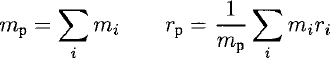
In order to clarify the accumulator that contains these two sums and the current sub-partition, we shall use a record type called accu:
> type accu = { mp: float; mprp: float; p: partition };;A function to compute the accumulator for a Leaf partition from a list of particles ps may be written:
> let make_leaf ps =
    let sum = List.fold_left (+) 0.0
    let m = List.map (fun p -> p.m) ps |> sum
    let mr = List.map (fun p -> p.m * p.r) ps |> sum
    {mp = m; mprp = mr; p = Leaf ps};;
val make_leaf : particle list -> accu
For example:
> make_leaf [{m = 1.0; r = −1.0}; {m = 3.0; r = l.o}];;
val it : accu =
  {mp = 4.0;
mprp = 2.0;
p = Leaf [{m = 1.0; r = −1.0;};
{m = 3.0; r = 1.0;}];}A function to compose two accumulators into a Node partition that includes a pseudo-particle approximant may be written:
> let make_node al a2 =
    let mp = al.mp + a2.mp
    let mprp = al.mprp + a2.mprp
    {mp = mp;
     mprp = mprp;
     p = Node(al.p, {m = mp; r = mprp / mp}, a2.p)};;
val make_node : accu -> accu -> accu
A particle system consists of the lower and upper bounds of the partition and the partition itself:
> type system =
    { lower: float; tree: partition; upper: float };;
The partition must be populated from a fiat list of particles. This can be done by recursively bisecting the range of the partition until either it contains 0 or 1 particles or until the range is very small:
> let rec partition xO ps x2 =
    match ps with
    | [] | [_] as ps -> make_leaf ps
    | ps when x2 - xO < epsilon_float -> make_leaf ps
    | ps ->
        let xl = (xO + x2) / 2.0
        let psl, ps2 =
          List.partition (fun p -> p.r < xl) ps
        make_node
          (partition xO psl xl) (partition xl ps2 x2);;
val partition : float -> particle list -> float -> accu
The List .partition function is used to divide the list of particles ps into those lying in the lower half of the range (ps1) and those lying in the upper half (ps2).
This partition function can be used to create a system from an array of particles:
> let rec make_system lower ps upper =
    {lower = lower;
     tree = (partition lower (List.of_seq ps) upper).p;
     upper = upper};;
val make_system :
  float -> particle array -> float -> system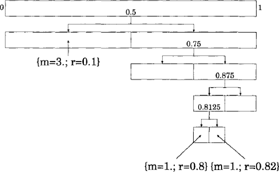
Figure 3.14. An unbalanced binary tree used to partition the space r ϵ (0,1) in order to approximate the gravitational effect of a cluster of particles in a system.
For example, consider the partition that results from 3 particles:
> let particles =
    [|{m = 3.0; r = O.l}; {m = 1.0; r = 0.8};
      {m = 1.0; r = 0.82} |];;
val particles : particle array

> make_system 0.0 particles 1.0;;
val it : system =
  {lower = 0.0;
   tree = Node (Leaf [{m = 3.0; r = 0.1;}],
           {m = 5.0; r = 0.384; },
           Node (Leaf null, {m = 2.0; r = 0.81;},
            Node
             (Node (Leaf [{m = 1.0; r = 0.8;}],
               {m = 2.0; r = 0.81;},
               Leaf [{m = 1.0; r = 0.82;}]),
             {m = 2.0; r = 0.81;}, Leaf null)));
   upper = 1.0;}
This tree is illustrated in figure 3.14. Note that the pseudo-particle at the root node of the tree correctly indicates that the total mass of the system ism = 3+l + l = 5 and the centre of mass is at
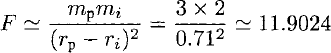
We shall now consider the force on the particle at r = 0.1, exerted by the other particles at r = 0.8 and 0.82. The force can be calculated exactly, in arbitrary units, as:
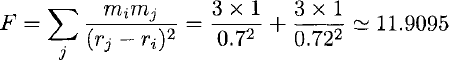
In this case, the force on the particle at ri = 0.1 can also be well-approximated by grouping the effect of the other two particles into that of a pseudo-particle. From the tree, the pseudo-particle for the range
wnere mp and r p are the mass and center of mass of the pseudo-particle, respectively.
Given the representation of a particle system as an unbalanced partition tree, the force on any given "origin" particle due to the particles in the system can be computed very efficiently by recursively traversing the tree either until a pseudo-particle in a non-leaf node is found to approximate the effects of the particles in its branch of the tree to sufficient accuracy or until real particles are found in a leaf node. This approach can be made more rigorous by bounding the error of the approximation.
The simplest upper bound of error is obtained by computing the difference between the minimum and maximum forces which can be obtained by a particle distribution satisfying the constraint that it must produce the pseudo-particle with the appropriate mass and position. Ifr i ∉ [X0, X2), the force F is bounded by the force due to masses at either end of the range and the force due to all the mass at the centre of mass:
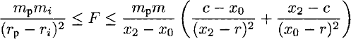
For example, the bounds of the force in the previous example are given by r = 0.1, m = 3, x0 = 0.5, c = 0.81, x2 = 1 and M = 2:
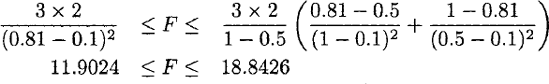
If this error was considered to be too large, the function approximating the total force would bisect the range and sum the contributions from each half recursively. In this case, the lower half contains no particles and the upper half [x1, X2) = [0.75,1) is considered instead. This tightens the bound on the force to:
This recursive process can be repeated either until the bound on the force is tight enough or until an exact result is obtained.
The following function computes the difference between the upper and lower bounds of the force on an origin particle p due to a pseudo-particle pp representing a particle distribution in the spatial range from xO to x2:
> let metric p pp xO x2 =
    if xO <= p.r && p.r < x2 then infinity else
    let sqr x = x * x
let fmin = p.m * pp.m / sqr (p.r - pp.r)
let g x y = (pp.r - x) / sqr(p.r - y)
let fmax =
p.m * pp.m / (x2 - xO) * (g xO x2 - g x2 xO)
fmax - fmin;;
val metric :
particle -> particle -> float -> float -> floatNote that the metric function returns an infinite possible error if the particle p lies within the partition range (X 0, X 2), as the partition might contain another particle at the same position
For example, these are the errors resulting from progressively finer approximations:
> metric { m = 3.0; r = 0.1 } { m = 2.0; r = 0.81 }
    0.0 1.0;;
val it : float = infinity

> metric {m=3.0; r = 0.1 } { m=2.0; r = 0.81 }
    0.5 1.0;;
val it : float = 6.94019227519524939

> metric { m = 3.0; r = 0.1 } { m = 2.0; r = 0.81 }
    0.75 1.0;;
val it : float = 0.668276868664461787

> metric { m = 3.0; r = 0.1 } { m = 2.0; r = 0.81 }
    0.75 0.875;;
val it : float = 0.277220270131675051
A function to compute an approximation to the total force on a particle p due to other particles in a system sys to within an error delta can be written:
> let rec force_aux xO x2 = function
    | Leaf list ->
        Seq.fold (fun f p2 -> f + force2 p p2) 0.0 list
    | Node(left, pp, right) ->
        if metric p pp xO x2 < delta then
          force2 p pp
        else
          let xl = 0.5 * (xO + x2)
          force_aux xO xl left + force_aux xl x2 right;;
val force_aux : float -> float ->
> let force p system delta =
    force_aux system.lower system.upper sys.tree;;
val force : particle -> system -> float -> float
The tree representation of this particle system is easily constructed by folding our insert function over the array which was used to test the array_force function:
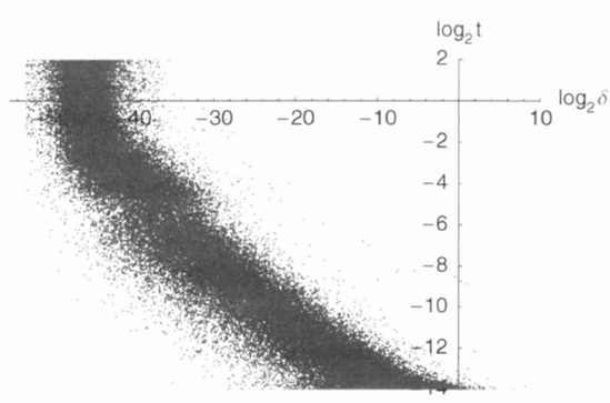
Figure 3.15. Measured performance of the tree-based approach relative to a simple array-based approach for the evaluation of long-range forces showing the resulting fractional error
> let system = make_system 0.0 system 1.0;;
val system : system
The tree-based force function can compute controllably accurate approximations to the force on an origin particle due to a collection of other particles, trading accuracy for performance.
Applying the force function with increasing permitted error results in a significant improvement in performance:
> force origin system le-9;;
val it : float = 2362356950.0

> force origin system le-6;;
val it : float = 2362356950.0

> force origin system le-3;;
val it : float = 2362356950.0
Moreover, the result does not change within 11 significant figures in this case!
From measurements of real-time performance (illustrated in figure 3.15), when requiring a force computation with an accuracy of one part in one million accuracy
The tree-based approach we have just described is a simple form of what is now known as the Fast Multipole Method (FMM) [23]. Before being applicable to most physical systems, the approaches we have described must be generalized to higher dimensionalities. This generalisation is most easily performed by increasing the branching factor of the tree from 2 to 2d for a d-dimensional problem. A more powerful generalisation involves associating the branches of the binary tree with subdivision along a particular dimension (either implicitly, typically by cycling through the dimensions, or explicitly, by storing the index of the subdivided dimension in the node of the tree). In particular, this allows anisotropic subdivision of space, i.e. some dimensions can be subdivided more than others. Anisotropic subdivision is useful in the context of anisotropic particle distributions, such as those found in many astrophysical simulations. One such method of anisotropic subdivision is known as the k-D tree.
Symbolic expressions can be represented very elegantly in F# as a form of tree known as an abstract syntax tree. This section describes a minimal implementation of symbolic expressions in F# and some simple functions to manipulate them.
Expressions composed of integers, variables, additions and multiplications may be represented by the variant type:
> type expr =
    | Int of int
    | Var of string
    | Add of expr * expr
    | Mul of expr * expr;;
For example, the following F# value represents the expression (1 + x) × 3:
> Mul(Add(Int 1, Var "x"), Int 3);;
val it : expr = Mul(Add(Int 1, Var "x"), Int 3);;
Such expressions can be manipulated using functions over the expr type. Before we delve into this area, it is useful to provide a more convenient way to construct symbolic expressions as well as a more convenient way to visualize them in the F# interactive mode.
Symbolic expressions may be constructed by overloading the + and * operators. This is done by supplementing the definition of the variant type expr with static member functions (described in section 2.4.1.3):
> type expr =
    | Int of int
    | Var of string
    | Add of expr * expr
    | Mul of expr * expr
    with
      static member (+) (f, g) = Add(f, g)
static member (-) (f, g) =
Add(f, Mul(Int(-1), g))
static member (*) (f, g) = Mul(f, g);;The previous example may be constructed more clearly using these infix operators:
> (Int 1 + Var "x") * Int 3;;
val it : expr = Mul(Add(Int 1, Var "x"), Int 3)
In this case, the arithmetic operators naively compose subexpressions. More intelligent constructors can be used to maintain a more sophisticated and efficient representation of symbolic mathematical expressions.
Perhaps the simplest function that acts upon a symbolic expression is one that evaluates the expression to get a value. Values of this expr type can be evaluated to the F# type int using the following eval function:
> let rec eval vars = function
    | Int n -> n
    | Var v -> List.assoc v vars
    | Add(f, g) -> eval vars f + eval vars g
    | Mul(f, g) -> eval vars f * eval vars g;;
val eval : (string * int) list -> expr -> int
The argument vars is an association list giving the values of variables that might appear in the expression being evaluated.
For example, the expression (1 + x) × 3 may be evaluated in the context x = 2 to get (l + 2) × 3 = 9:
> eval ["x", 2] ((Int 1 + Var "x") * Int 3);;
val it : int = 9
By defining another variant type (typically called value) to represent the kinds of values that can result from evaluation, this approach can be generalized to evaluate more complicated expressions containing different kinds of numbers and even strings, compound types and functions. When expressions can define and apply arbitrary functions, this eval function becomes an interpreter for a simple programming language [14]. Many programming languages are implemented in this way and domain-specific languages have a variety of applications in scientific computing.
Another important use of symbolic expressions is rewriting them to produce related expressions. This approach is often known as term rewriting and involves repeated applications of sets of rewrite rules designed to transform an expression into a different (but typically equivalent) form.
A higher-order rewrite function can be used to implement generic term rewriting:
> let rec rewrite rule expr =
let expr' =
      match expr with
      | Int _ | Var _ as f -> rule f
      | Add(f, g) ->
          rule(rewrite rule f + rewrite rule g)
      | Mul(f, g) ->
          rule(rewrite rule f * rewrite rule g)
    if expr = expr' then expr else rewrite rule expr';;
val rewrite : (expr -> expr) -> expr -> expr
This rewrite function takes a function rule that transforms expressions and applies it to every subexpression of the given expression. For example, using rewrite to apply the identity rule to the expression 3 + x will apply the rule to the subexpressions 3, then x and then the whole expression 3 + x. This rewrite function continues rewriting until the expression stops changing.
The rewrite rule (f + g) × h → f × h + g × h can be used to expand products of sums and may be written:
> let rec expand = function
    | Mul(Add(f, g), h) | Mul(h, Add(f, g)) ->
        f * h + g * h
    | f -> f;;
val expand : expr -> expr
Note that F# does not know that Mul (f, g) and Mul (g, f) are equivalent, so we are careful to account for both alternatives in the pattern.
For example, the rewrite and expand functions may be used to expand the expression (1 + x) × 3 to 1 × 3 + x × 3:
> rewrite expand ((Int 1 + Var "x") * Int 3);;
val it : expr =
  Add(Mul(Int 1, Int 3), Mul(Var "x", Int 3))
Symbolic computations are of increasing importance in scientific computing and the ML family of languages are very powerful tools for such work, with existing applications ranging from accumulating contributions from billions of Feynman graphs in string theory [6] to the generation of the high-performance FFT implementations in software such as MATLAB [9].
We shall revisit the handling of symbolic expressions in F# later in this book, in the context of parsing (section 5.5.2), metaprogramming (section 9.12) andinteroperating with computer algebra systems (section 11.3).
[10] Average-case complexity is particularly useful when statistics are available on the likelihood ofdifferent inputs.
[11] Balanced binary trees will be discussed in more detail later in section 3.10.
[12] Computingthe hash in
[13] Not to be confused with the higher-order map function provided with many data structures.
[14] 1f only zero or one "branches" are allowed at each node then the tree is actually a list (see section 3.8).
[15] Although taking limits over integer-valued variables may seem dubious, the required proofs can, in fact, be made rigorous.