
Chapter 2. Two State Economy
As an empirical domain, finance is aimed at specific answers, such as an appropriate value for a given security, or an optimal number of its shares to hold.
Darrell Duffie (1988)
The notion of arbitrage is crucial to the modern theory of Finance.
Delbaen and Schachermeyer (2006)
The analysis in this chapter is based on the most simple model economy that is still rich enough to introduce many important notions and concepts of finance: an economy with two relevant points in time and two uncertain future states only. It also allows to present some important results in the field, like the Fundamental Theorems of Asset Pricing that are discussed in this chapter.1
The simple model chosen is a means to simplify the formal introduction of the sometimes rather abstract mathematical concepts and financial ideas by avoiding as many technicalities as possible. Once these ideas are fleshed out and well understood, the transfer to more realistic financial models usually proves seamless.
This chapter covers mainly the following central topics from finance, mathematics, and Python programming.
| Finance | Mathematics | Python |
|---|---|---|
time |
natural numbers |
|
money (currency) |
real numbers |
|
cash flow |
tuple |
|
return, interest |
real numbers |
|
(net) present value |
function |
|
uncertainty |
vector |
|
financial asset |
process |
|
risk |
probability, state space, power set, mapping |
|
expectation, expected return |
dot product |
|
volatility |
variance, standard deviation |
|
contingent claims |
random variable |
|
replication, arbitrage |
linear equations, matrix form |
|
completeness, Arrow-Debreu securities |
linear independence, span |
|
martingale pricing |
martingale, martingale measure |
|
mean-variance |
expectation, variance, standard deviation |
|
Economy
The first element of the financial model is the idea of an economy. An economy is an abstract notion which subsumes other elements of the financial model, like assets (real, financial), agents (people, institutions) or currency. Like in the real world, an economy cannot be seen or touched. Nor can it be formally modeled directly — it rather simplifies communication to have such a summary term available. The single model elements together form the economy.
Real Assets
Multiple real assets are available in the economy that can be used for different purposes. A real asset might be a chicken egg or a complex machine to produce other real assets. At this point it is not yet relevant who, for example, produces the real assets or who owns them.
Agents
Agents can be thought of as individual human beings being active in the economy. They might be involved in producing real assets, consuming them or trading them. They accept money during transactions and spend it during others. An agent might also be an institution like a bank that allows other agents to deposit money on which it then pays interest.
Time
Economic activity, like trading real assets, takes place at discrete points in time only. Formally, it holds for a point in time
The Python data type to model the natural numbers int which stands for integers.2 Typical arithmetic operations are possible on integers like addition, subtraction, multiplication and more.
In[1]:1+3Out[1]:4In[2]:3*4Out[2]:12In[3]:t=0In[4]:tOut[4]:0In[5]:t=1In[6]:type(t)Out[6]:int

Adds up two integer values.

Multiplies two integer values.

Assigns a value of 0 to the variable name
t.
Prints out the value of variable
t.
Assigns a new value of 1 to
t.
Looks up and prints the Python type of
t.
Money
In the economy, there is money (or currency) in unlimited supply available. Money is also infinitely divisible. Money and currency should be thought of in abstract terms only and not in terms of cash (physical coins or bills).
Money in general serves as the numeraire in the economy in that the value of one unit of money (think USD, EUR, GBP, etc.) is normalized to exactly 1. The prices for all other goods are then expressed in such units and are fractions or multiples of such units. Formally, units of the currency are represented as (positive) real numbers
In Python, float is the standard data type used to represent real numbers int type, it allows, among others, for typical arithmetic operations, like addition and subtraction.
In[7]:1+0.5Out[7]:1.5In[8]:10.5-2Out[8]:8.5In[9]:c=2+0.75In[10]:cOut[10]:2.75In[11]:type(c)Out[11]:float
Adding two numbers.
Subtracting two numbers.
Assigning the result of the addition to the variable name
c.Printing the value of the variable
c.Looking up and printing out the Python type of the variable
c.
Beyond serving as a numeraire, money also allows to buy and sell real assets or to store value over time. These two functions rest on the trust that money has indeed intrinsic value today and also in one year. In general, this translates into trust in people and institutions being willing to accept money both today and later for any kind of transaction. The numeraire function is independent of this trust since it is a numerical operation only.
Cash Flow
Combining time with currency leads to the notion of cash flow. Consider an investment project which requires an investment of, say, 9.5 currency units today and pays back 11.75 currency units after one year. An investment is generally considered to be a cash outflow and one often represents this as a negative real number,
To indicate the points in time when cash flows happen, a time index is used. In the example,
A pair of cash flows now and one year from now is modeled mathematically as an ordered pair or two-tuple which combines the two relevant cash flows to one object
In Python, there are multiple data structures available to model such a mathematical object. The two most basic ones are tuple and list. Objects of type tuple are immutable, i.e. they cannot be changed after instantiation, while those of type list are mutable and can be changed after instantiation. First, an illustration of tuple objects (characterized by parentheses or round brackets).
In[12]:c0=-9.5In[13]:c1=11.75In[14]:c=(c0,c1)In[15]:cOut[15]:(-9.5,11.75)In[16]:type(c)Out[16]:tupleIn[17]:c[0]Out[17]:-9.5In[18]:c[1]Out[18]:11.75
Defines the cash outflow today.
Defines the cash inflow one year later.
Defines the
tupleobjectc(note the use of parentheses).Prints out the cash flow pair (note the parentheses).
Looks up and shows the type of object
c.Accesses the first element of object
c.
Accesses the second element of object
c.
Second, an illustration of the list object (characterized by square brackets).
In[19]:c=[c0,c1]In[20]:cOut[20]:[-9.5,11.75]In[21]:type(c)Out[21]:listIn[22]:c[0]Out[22]:-9.5In[23]:c[1]Out[23]:11.75In[24]:c[0]=10In[25]:cOut[25]:[10,11.75]
Defines the
listobjectc(note the use of square brackets).Prints out the cash flow pair (note the square brackets).
Looks up and shows the type of object
c.Accesses the first element of object
c.Accesses the second element of object
c.Overwrites the value at the first index position in the object
c.Shows the resulting changes.
Return
Consider an investment project with cash flows
In Python, this boils down to simple arithmetic operations.
In[26]:c=(-10,12)In[27]:R=sum(c)In[28]:ROut[28]:2In[29]:r=R/abs(c[0])In[30]:rOut[30]:0.2
Defines the cash flow pair as
tupleobject.Calculates the return
Rby taking the sum of all elements ofcand …… prints out the result.
Calculates the rate of return
rwithabs(x)giving the absolute value ofxand …… prints out the result.
Interest
There is a difference between a cash flow today and a cash flow in one year. The difference results from interest that is being earned on currency units or that has to be paid to borrow currency units. Interest in this context is the price being paid for having control over money that belongs to another agent.
An agent that has currency units that they do not need today can deposit these with a bank or lend them to another agent to earn interest. If the agent needs more currency units than they have currently available, they can borrow them from a bank or other agents and needs to pay interest.
Suppose an agent deposits
In the following, it is assumed that the relevant interest rate for both lending and borrowing is the same and that it is fixed for the entire economy.
Present Value
Having lending or depositing options available leads to opportunity costs for deploying money in an investment project. A cash flow of, say,
To appropriately compare cash flows in one year with those of today, the present value needs to be calculated. This is accomplished by discounting using the fixed interest rate in the economy. Discounting can be modeled as a function
for an interest rate of
Python functions are well suited to represent mathematical functions like the one for discounting.
In[31]:i=0.1In[32]:defD(c1):returnc1/(1+i)In[33]:D(12.1)Out[33]:10.999999999999998In[34]:D(11)Out[34]:10.0
Fixes the interest rate
i.Function definition with
defstatement;Dis the function name;c1the parameter name.Returns the present value with the
returnstatement.Calculates the present value of 12.1; note the rounding error due to internal float point number representation issues.
Calculates the present value of 11 (“exactly” in this case).
Net Present Value
How shall an agent decide whether to conduct an investment project or not? One criterion is the net present value. The net present value
Consider an investment project with cash flows
Building on previous definitions, a respective Python function is easily defined.
In[35]:defNPV(c):returnc[0]+D(c[1])In[36]:cA=(-10.5,12.1)In[37]:cB=(-10.5,11)In[38]:NPV(cA)Out[38]:0.4999999999999982In[39]:NPV(cB)Out[39]:-0.5
Positive net present value project.
Negative net present value project.
Uncertainty
Cash inflows from an investment project one year from now are in general uncertain. They might be influenced by a number of factors in reality (competitive forces, new technologies, growth of the economy, weather, problems during project implementation, etc.). In the model economy, the concept of states of the economy in one year subsumes the influence of all relevant factors.
Assume that in one year the economy might be in one of two different states
Mathematically, there are multiple operations defined on such vectors, like scalar multiplication and addition, for instance.
Another important operation on vectors are linear combinations of vectors. Consider two different vectors
Here and before, it is assumed that
The most common way of modeling vectors (and matrices) in Python, is via the NumPy package which is an external package and needs to be installed separately. For the code below, consider an investment project with ndarray class which stands for n-dimensional array.
In[40]:importnumpyasnpIn[41]:c0=-10In[42]:c1=np.array((20,5))In[43]:type(c1)Out[43]:numpy.ndarrayIn[44]:c1Out[44]:array([20,5])In[45]:c=(c0,c1)In[46]:cOut[46]:(-10,array([20,5]))In[47]:1.5*c1+2Out[47]:array([32.,9.5])In[48]:c1+1.5*np.array((10,4))Out[48]:array([35.,11.])
Imports the
numpypackage asnp.The cash outflow today.
The uncertain cash inflow in one year; one-dimensional
ndarrayobjects do not distinguish between row (horizontal) and column (vertical).Looks up and prints the type of
c1.Prints the cash flow vector.
Combines the cash flows to a
tupleobject.tuplelikelistobjects can contain other complex data structures.
A linear transformation of the vector by scalar multiplication and addition; technically one also speaks of a vectorized numerical operation and of broadcasting.

A linear combination of two
ndarrayobjects (vectors).
Financial Assets
Financial assets are financial instruments (“contracts”) that have a fixed price today and an uncertain price in one year. Think of share in the equity of a firm that conducts an investment project. Such a share might be available at a price today of
One speaks also of the price process of the financial asset
The NumPy package is again the tool of choice for the modeling.
In[49]:S0=10In[50]:S1=np.array((12.5,7.5))In[51]:S=(S0,S1)In[52]:SOut[52]:(10,array([12.5,7.5]))In[53]:S[0]Out[53]:10In[54]:S[1][0]Out[54]:12.5In[55]:S[1][1]Out[55]:7.5
The price of the financial asset today.
The uncertain price in one year as a vector (
ndarrayobject).The price process as a
tupleobject.Prints the price process information.
Accesses the price today.
Accesses the price in one year in the
Accesses the price in one year in the
Risk
Often it is implicitly assumed that the two states of the economy are equally likely. What this means in general is that when an experiment in the economy is repeated (infinitely) many times, it is observed that half of the time the
This is a frequentist point of view, according to which probabilities for a state to materialize are calculated based on the frequency the state is observed divided by the total number of experiments leading to observations. If state
In a modeling context, the probabilities for all possible states to occur are assumed to be given a priori. One speaks sometimes of objective or physical probabilities.
Probability Measure
The probabilities for events that are physically possible together form a probability measure. Such a probability measure is a function
A function
The first condition implies that at least one of the states must materialize. The second implies that the probability for a state to materialize is between 0 and 1. The third one says that all the probabilities add up to 1.
In the simple model economy with two states only, it is convenient to define
Having a fully specified probability measure available, the model economy is typically called an economy under risk. A model economy without a fully specified probability measure is often called an economy under ambiguity.
In applications, a probability measure is usually modeled also as a vector and ndarray object, respectively. This is at least possible for a discrete state space with a finite number of elements.
In[56]:p=0.4In[57]:1-pOut[57]:0.6In[58]:P=np.array((p,1-p))In[59]:POut[59]:array([0.4,0.6])
Notions of Uncertainty
Uncertainty in a financial context can take on different forms. Risk in general refers to a situation in which a full probability distribution over future states of the economy is (assumed to be) known. Ambiguity refers to situations in which such a distribution is not known. Traditionally, finance has relied almost exclusively on model economies under risk, although there is a stream of research that deals with finance problems under ambiguity (see Guidolin and Rinaldi (2012) for a survey of the research literature).
Expectation
Based on the probability measure, the expectation of an uncertain quantity, like the price in one year of a financial asset, can be calculated. The expectation can be interpreted as the weighted average where the weights are given by the probabilities. It is an average since the probabilities add up to one.
Consider the financial asset with price process
with
Mathematically, the expectation can be expressed as the dot product (or inner product) of two vectors. If
Therefore, with
Working with ndarray objects in Python, the dot product is defined as a function provided by the NumPy package.
In[60]:POut[60]:array([0.4,0.6])In[61]:S0=10In[62]:S1=np.array((20,5))In[63]:np.dot(P,S1)Out[63]:11.0
The previously defined probability measure.
The price of the financial asset today.
The vector of the uncertain price in one year.
The dot product of the two vectors calculating the expectation value.
Expected Return
Under uncertainty, the notions of return and rate of return need to be adjusted. In such a case, the expected return of a financial asset is given as the expectation of the price in one year minus the price today. This can be seen by taking the expectation of the uncertain return
With the assumptions from before, one gets
The expected rate of return then simply is the expected return divided by the price today
which can be also derived step-by-step with similar transformations as for the expected return. In what follows, the expected rate of return is symbolized by
The calculation of expected return and rate of return can be modeled in Python by two simple functions.
In[64]:defER(x0,x1):returnnp.dot(P,x1)-x0In[65]:ER(S0,S1)Out[65]:1.0In[66]:defmu(x0,x1):return(np.dot(P,x1)-x0)/x0In[67]:mu(S0,S1)Out[67]:0.1
Definition of expected return.
The expected return for the previously defined financial asset.
Definition of the expected rate of return.
The expected rate of return calculate for that asset.
Volatility
In finance, risk and expected return is the dominating pair of concepts. Risk can be measured in many ways, while the volatility measured as the standard deviation of the rates of return is probably the most common measure. In the present context, the variance of the return rates of a financial asset is defined by
with
Python functions modeling these two risk measures are given below. Also a helper function to calculate the return rates vector.
In[68]:defr(x0,x1):return(x1-x0)/x0In[69]:r(S0,S1)Out[69]:array([1.,-0.5])In[70]:mu=np.dot(P,r(S0,S1))In[71]:muOut[71]:0.10000000000000003In[72]:defsigma2(P,r,mu):returnnp.dot(P,(r-mu)**2)In[73]:sigma2(P,r(S0,S1),mu)Out[73]:0.54In[74]:defsigma(P,r,mu):returnnp.sqrt(np.dot(P,(r-mu)**2))In[75]:sigma(P,r(S0,S1),mu)Out[75]:0.7348469228349535
Vectorized calculation of the rates of return vector.
Applies the function to the financial asset from before.
The expected rate of return via the dot product …
… printed out.
The definition of the variance of the rates of return.
The function applied to the rates of return vector.
The definition of the volatility.
And applied to the rates of return vector.
Vectors, Matrices and NumPy
Finance as an applied mathematical discipline relies heavily on linear algebra and probability theory. In the discrete model economy, both mathematical disciplines and be efficiently handled in Python by using the NumPy package with its powerful ndarray object. This is not only true from a modeling point of view but also from handling, calculation, optimization, visualization and other points of view. Basically all examples to follow in the book will support these claims.
Contingent Claims
Suppose now that a contingent claim is traded in the economy. This is a financial asset — formalized by some contract — that offers a state-contingent payoff one year from now. Such a contingent claim can have an arbitrary state-contingent payoff or one that is derived from the payoff of other financial assets. In the latter case, one generally speaks of derivative assets or derivatives instruments. Formally, a contingent claim is a function
Assume that two financial assets are traded in the economy. A risk-less bond with price process
In probability theory, a contingent claim is usually called a random variable whose defining characteristic is that it maps elements of the state space to real numbers — potentially via other random variables as is the case for derivative assets. In that sense, the price of the stock in one year
For the sake of illustration, the Python code below visualizes the payoff of a call option on a segment of the real line. In the economy, there are of course only two states — and therewith two values — of relevance. Figure 2-1 shows the payoff function graphically.
In[76]:S1=np.arange(20)In[77]:S1[:7]Out[77]:array([0,1,2,3,4,5,6])In[78]:K=10In[79]:C1=np.maximum(S1-K,0)In[80]:C1Out[80]:array([0,0,0,0,0,0,0,0,0,0,0,1,2,3,4,5,6,7,8,9])In[81]:frompylabimportmpl,plt# plotting configurationplt.style.use('seaborn')mpl.rcParams['savefig.dpi']=300mpl.rcParams['font.family']='serif'In[82]:plt.figure(figsize=(10,6))plt.plot(S1,C1,lw=3.0,label='$C_1 =max(S_1 - K, 0)$')plt.legend(loc=0)plt.xlabel('$S_1$')plt.ylabel('$C_1$');
Generates an
ndarrayobject with numbers from 0 to 19.Shows the the first few numbers.
Fixes the strike price for the call option.
Calculates in vectorized fashion the call option payoff values.
Shows these values — many values are 0.
Imports the main plotting sub-package from
matplotlib.Plots the call option payoff against the stock values; sets the line width to 3 pixels and defines a label as a string object with
Latexcode.Puts the legend in the optimal location (least overlap with plot elements).
Places a label on the
xaxis …
… and on the
yaxis.

Figure 2-1. Payoff of the call option
Replication
When introducing a contingent claim into the economy, an important question that arises is whether the payoff of the contingent claim is redundant or not. Mathematically, one speaks of the payoff vector of the contingent claim being linearly dependent or linearly independent.
The payoff of the call option is said to be linearly dependent — or redundant — when a solution to the following problem exists for
with
This problem can be represented as a system of linear equations
With
and
Assume as before that two financial assets are traded, a risk-less bond
and
In words, buying one third of the stock and selling
Technically, short selling implies borrowing the respective number of units of the financial asset today from another agent and immediately selling it in the market. In one year, the borrowing agent buys the exact number of units of the financial asset back in the market to the then current price and transfers them back to the other agent.
The analysis here assumes that all financial assets — like money — are infinitely divisible which might not be the case in practice. It also assumes that short selling of all traded financial assets is possible which might not be too unrealistic given market practice.
As a preparation for the implementation in Python, consider yet another way of formulating the replication problem. To this end, the mathematical concept of a matrix is needed. While a vector is a one-dimensional object, a matrix is a two-dimensional object. For the purposes of this section, consider a square matrix
The future payoff vectors of the bond and the stock represent the values in the first and second column of the matrix, respectively. The first row contains the payoff of both financial assets in the state
where
In this context, matrix multiplication is defined by
which shows the equivalence between this way of representing the replication problem and the one from before.
The ndarray class allows for a modeling of matrices in Python. The NumPy package provides in the sub-package np.linalg a wealth of functions for linear algebra operations among which there is also a function to solve systems of linear equations in matrix form — exactly what is needed here.
In[83]:B=(10,np.array((11,11)))In[84]:S=(10,np.array((20,5)))In[85]:M=np.array((B[1],S[1])).TIn[86]:MOut[86]:array([[11,20],[11,5]])In[87]:K=15In[88]:C1=np.maximum(S[1]-K,0)In[89]:C1Out[89]:array([5,0])In[90]:phi=np.linalg.solve(M,C1)In[91]:phiOut[91]:array([-0.15151515,0.33333333])
Defines the price process for the risk-less bond.
Defines the price process for the risky stock.
Defines a matrix — i.e. a two-dimensional
ndarrayobject — with the future payoff vectors.Shows the matrix with the numerical values.
Fixes the strike price for the call option and …
… calculates the values for the payoff vector in one year.
Shows the numerical values of the payoff vector.
Solves the replication problem in matrix form to obtain the optimal portfolio positions.
Arbitrage Pricing
How much does it cost to replicate the payoff of the call option? Once the portfolio to accomplish the replication is derived, this question is easy to answer. Define the value of the replication portfolio today by
or in numbers
The uncertain value of the replication portfolio in one year
Together, one has the value process of the portfolio as
Having a portfolio available that perfectly replicates the future payoff of a contingent claim raises the next question: what if the price of the contingent claim today differs from the costs of setting up the replication portfolio? The answer is simple but serious: then there exists an arbitrage or arbitrage opportunity in the economy. An arbitrage is a trading strategy
-
-
Suppose that the price of the call option is
by the definition of the replication portfolio. In the other case, when the price of the call option today is lower than the price of the replication portfolio, say
A model for an economy which allows for arbitrage opportunities can be considered not viable. Therefore the only price that is consistent with the absence of arbitrage is
Formally, the arbitrage price is the dot product of the replication portfolio and the price vector of the replicating financial assets
giving rise to an arbitrage-free price process for the contingent claim of
In Python, this is a single calculation given the previous definitions and calculations.
In[92]:C0=np.dot(phi,(B[0],S[0]))In[93]:C0Out[93]:1.8181818181818183In[94]:10/3-50/33Out[94]:1.8181818181818183
Market Completeness
Does arbitrage pricing work for every contingent claim? Yes, at least for those that are replicable by portfolios of financial assets that are traded in the economy. The set of attainable contingent claims
if short-selling is prohibited and
if it is allowed in unlimited fashion.
Consider the risk-less bond and the risky stock from before with price processes
has a unique solution for any
and consequently as
which was derived in the context of the replication of the special call option payoff. The solution carries over to the general case since no special assumptions have been made regarding the payoff other than
Since every contingent claim can be replicated by a portfolio consisting of a position in the risk-less bond and the risky stock, one speaks of a complete market model. Therefore, every contingent claim can be priced by replication and arbitrage. Formally, the only requirement being that the price vectors of the two financial assets in one year be linearly independent. This implies that
has only the unique solution
The spanning property can be visualized by the use of Python and the matplotlib package. To this end, 1,000 random portfolio compositions are simulated. The first restriction is that the portfolio positions should be positive and add up to 1. Figure 2-2 shows the result.
In[95]:np.random.seed(100)In[96]:n=1000In[97]:b=np.random.random(n)In[98]:b[:5]Out[98]:array([0.54340494,0.27836939,0.42451759,0.84477613,0.00471886])In[99]:s=(1-b)In[100]:s[:5]Out[100]:array([0.45659506,0.72163061,0.57548241,0.15522387,0.99528114])In[101]:defportfolio(b,s):A=[b[i]*B[1]+s[i]*S[1]foriinrange(n)]returnnp.array(A)In[102]:A=portfolio(b,s)In[103]:A[:3]Out[103]:array([[15.10935552,8.26042965],[17.49467553,6.67021631],[16.17934168,7.54710554]])In[104]:plt.figure(figsize=(10,6))plt.plot(A[:,0],A[:,1],'r.');
Fixes the seed for the random number generator.
Number of values to be simulated.
Simulates the bond position for values between 0 and 1 by the means of a uniform distribution.
Derives the stock position as the difference between 1 and the bond position.
This calculates the portfolio payoff vectors for all random portfolio compositions and collects them in a
listobject; this Python idiom is called alistcomprehension.The function returns a
ndarrayversion of the results.The calculation is initiated.
The results are plotted.

Figure 2-2. The random portfolios span a one-dimensional line only
Figure 2-3 shows the graphical results in the case where the portfolio positions do not need to add up to 1.
In[105]:s=np.random.random(n)In[106]:b[:5]+s[:5]Out[106]:array([0.57113722,0.66060665,1.3777685,1.06697466,0.30984498])In[107]:A=portfolio(b,s)In[108]:plt.figure(figsize=(10,6))plt.plot(A[:,0],A[:,1],'r.');
The stock position is freely simulated for values between 0 and 1.
The portfolio payoff vectors are calculated.

Figure 2-3. The random portfolios span a two-dimensional area (rhomb)
Finally, Figure 2-4 allows for positive as well as negative portfolio positions for both the bond and the stock. The resulting portfolio payoff vectors cover an (elliptic) area around the origin.
In[109]:b=np.random.standard_normal(n)In[110]:s=np.random.standard_normal(n)In[111]:b[:5]+s[:5]Out[111]:array([-0.66775696,1.60724747,2.65416419,1.20646469,-0.12829258])In[112]:A=portfolio(b,s)In[113]:plt.figure(figsize=(10,6))plt.plot(A[:,0],A[:,1],'r.');
Positive and negative portfolio positions are simulated by the means of the standard normal distribution.

Figure 2-4. The random portfolios span a two-dimensional area (around the origin)
If
Arrow-Debreu Securities
An Arrow-Debreu security is defined by the fact that is pays exactly one unit of currency in a specified future state. In a model economy with two different future states only, there can only be two different such securities. An Arrow-Debreu security is simply a special case of a contingent claim such that the replication argument from before applies. In other words, since the market is complete Arrow-Debreu securities can be replicated by portfolios in the bond and stock. Therefore, both replication problems have (unique) solutions and both securities have unique arbitrage prices. The two replication problems are
and
Why are these securities important? Mathematically, the two payoff vectors form a standard basis or natural basis for the
The process is to first derive the replication portfolios for the two Arrow-Debreu securities and the resulting arbitrage prices for both. Other contingent claims are then replicated and priced based on the standard basis and the arbitrage prices of the two securities.
Consider the two Arrow-Debreu securities with price processes
Consider a general contingent claim with future payoff vector
The replication portfolio
Consequently, the arbitrage price for the contingent claim is
This illustrates how the introduction of Arrow-Debreu securities simplifies contingent claim replication and arbitrage pricing.
Martingale Pricing
A martingale measure
If
One also speaks of the fact that the price processes drift (on average) with the risk-less interest rate under the martingale measure
Denote
or after some simple manipulations
Given previous assumptions, for
What if these relationships for
If equality holds in these relationships one also speaks of a weak arbitrage since the risk-less profit can only be expected on average and not with certainty.
Assuming the numerical price processes from before, the calculation of
In[114]:i=(B[1][0]-B[0])/B[0]In[115]:iOut[115]:0.1In[116]:q=(S[0]*(1+i)-S[1][1])/(S[1][0]-S[1][1])In[117]:qOut[117]:0.4
First Fundamental Theorem of Asset Pricing
The considerations at the end of the previous section hint already towards a relationship between martingale measures on the one hand and arbitrage on the other. A central result in mathematical finance that relates these seemingly unrelated concepts formally is the First Fundamental Theorem of Asset Pricing. Pioneering work in this regard has been published by Cox and Ross (1976), Harrison and Kreps (1979) and Harrison and Pliska (1981).
First Fundamental Theorem of Asset Pricing (1FTAP)
The following statements are equivalent:
-
A martingale measure exists.
-
The economy is arbitrage-free.
Given the calculations and the discussion from before, the theorem is easy to prove for the model economy with the risk-less bond and the risky stock.
First, 1. implies 2.: If the martingale measure exists, the price processes do not allow for simple (weak) arbitrages. Since the two future price vectors are linearly independent, every contingent claim can be replicated by trading in the two financial assets implying unique arbitrage prices. Therefore, no arbitrages exist.
Second, 2. implies 1.: If the model economy is arbitrage-free, a martingale measure exists as shown above.
Pricing by Expectation
A corollary of the 1FTAP is that any attainable contingent claim
In other words, the discounted price process of the call option — and any other contingent claim — is a martingale under the martingale measure such that
In Python, the martingale pricing boils down to the evaluation of a dot product.
In[118]:Q=(q,1-q)In[119]:np.dot(Q,C1)/(1+i)Out[119]:1.8181818181818181
Defines the martingale measure as the tuple
Q.Implements the martingale pricing formula.
Second Fundamental Theorem of Asset Pricing
There is another important result, often called the Second Fundamental Theorem of Asset Pricing, which relates the uniqueness of the martingale measure with market completeness.
Second Fundamental Theorem of Asset Pricing (2FTAP)
The following statements are equivalent:
-
The martingale measure is unique.
-
The market model is complete.
The result also follows for the simple model economy from previous discussions. A more detailed analysis of market completeness takes place in Chapter 3.
Mean-Variance Portfolios
A major breakthrough in finance has been the formalization and quantification of portfolio investing through the mean-variance portfolio theory (MVP) as pioneered by Markowitz (1952). To some extent this approach can be considered to be the beginning of quantitative finance, initiating a trend that brought more and more mathematics to the financial field.
MVP reduces a financial asset to the first and second moment of its returns, namely the mean as the expected rate of return and the variance of the rates of return or the volatility defined as the standard deviation of the rates of return. Although the approach is generally called “mean-variance” it is often the combination “mean-volatility” that is used.
Consider the risk-less bond and risky stock from before with price processes
The expected portfolio payoff is
In words, the expected portfolio payoff is simply
Defining
one gets for the expected portfolio rate of return
In words, the expected portfolio rate of return is
The next step is to calculate the portfolio variance
In words, the portfolio variance is
The whole analysis is straightforward to implement in Python. First, some preliminaries.
In[120]:B=(10,np.array((11,11)))In[121]:S=(10,np.array((20,5)))In[122]:M=np.array((B[1],S[1])).TIn[123]:MOut[123]:array([[11,20],[11,5]])In[124]:M0=np.array((B[0],S[0]))In[125]:R=M/M0-1In[126]:ROut[126]:array([[0.1,1.],[0.1,-0.5]])In[127]:P=np.array((0.5,0.5))
The matrix with the future prices of the financial assets.
The vector with the prices of the financial assets today.
Calculates in vectorized fashion the return matrix.
Shows the results of the calculation.
Defines the probability measure.
With these definitions, expected portfolio return and volatility are calculated as dot products.
In[128]:np.dot(P,R)Out[128]:array([0.1,0.25])In[129]:s=0.55In[130]:phi=(1-s,s)In[131]:mu=np.dot(phi,np.dot(P,R))In[132]:muOut[132]:0.18250000000000005In[133]:sigma=s*R[:,1].std()In[134]:sigmaOut[134]:0.41250000000000003
The expected returns of the bond and the stock.
An example allocation for the stock in percent (decimals).
The resulting portfolio with a normalized weight of 1.
The expected portfolio return given the allocations.
The value lies between the risk-less return and the stock return.
The volatility of the portfolio; the Python code here only applies due to
Again, the value lies between the volatility of the bond (= 0) and the volatility of the stock (= 0.75).
Varying the weight of the stock in the portfolio leads to different risk-return combinations. Figure 2-5 shows the expected portfolio return and volatility for different values of
In[135]:values=np.linspace(0,1,25)In[136]:mu=[np.dot(((1-s),s),np.dot(P,R))forsinvalues]In[137]:sigma=[s*R[:,1].std()forsinvalues]In[138]:plt.figure(figsize=(10,6))plt.plot(values,mu,lw=3.0,label='$mu_p$')plt.plot(values,sigma,lw=3.0,label='$sigma_p$')plt.legend(loc=0)plt.xlabel('$s$');
Generates an
ndarrayobject with 24 evenly space intervals between 0 and 1.Calculates for every element in
valuesthe expected portfolio return and stores them in alistobject.Calculates for every element in
valuesthe portfolio volatility and stores them in anotherlistobject.

Figure 2-5. Expected portfolio return and volatility for different allocations
Note that the list comprehension sigma = [s * R[:, 1].std() for s in values] in the code above is short for the following code3:
sigma=list()forsinvalues:sigma.append(s*R[:,1].std())
The typical graphic seen in the context of MVP is one that plots expected portfolio return against portfolio volatility. Figure 2-6 shows that an investor can expect a higher return the more risk (volatility) she is willing to bear. The relationship is linear in the special case of this section.
In[139]:plt.figure(figsize=(10,6))plt.plot(sigma,mu,lw=3.0,label='risk-return')plt.legend(loc=0)plt.xlabel('$sigma_p$')plt.ylabel('$mu_p$');
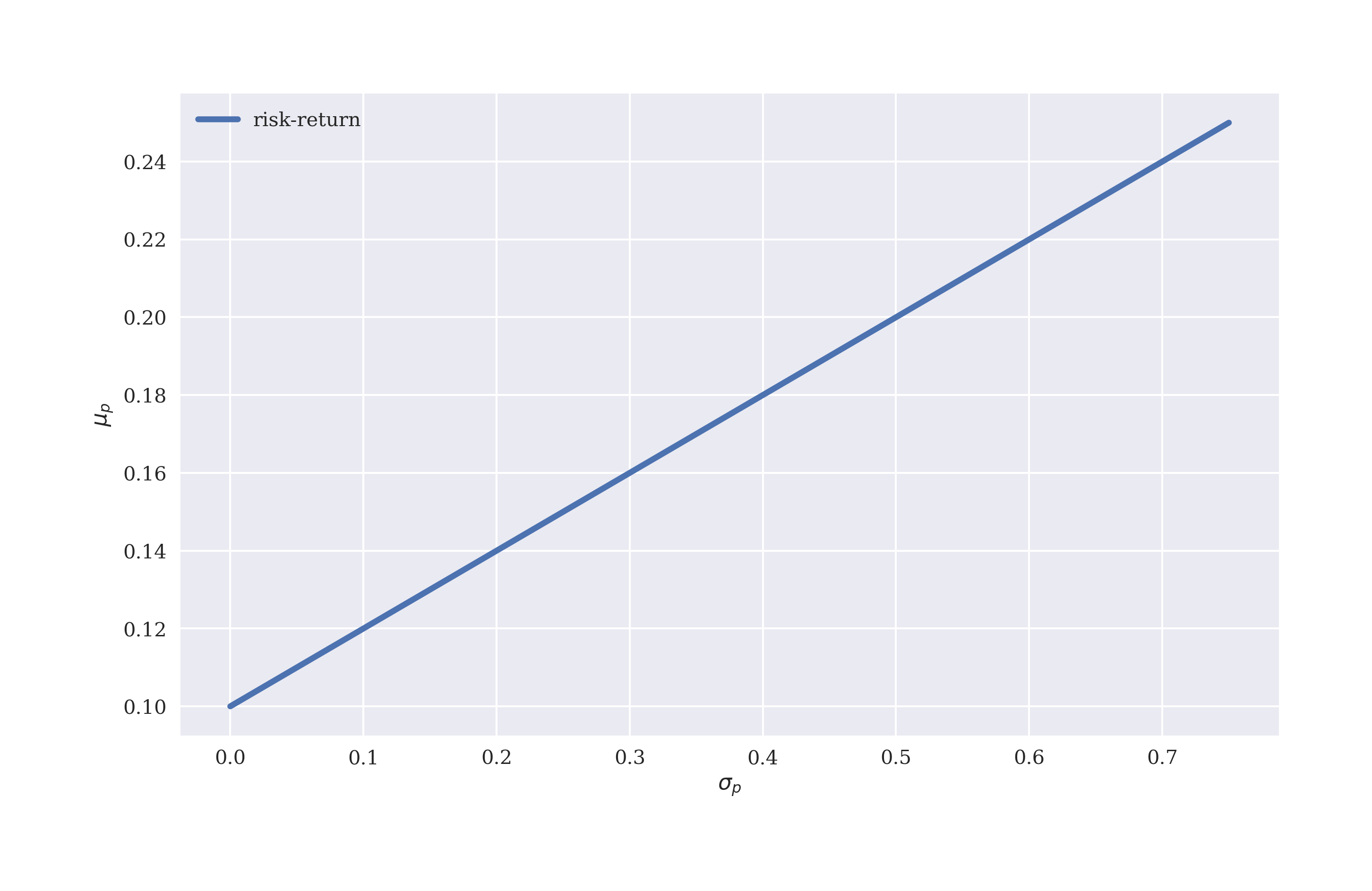
Figure 2-6. Feasible combinations of expected portfolio return and volatility
Conclusions
This chapter introduces to finance, starting with the very basics and illustrating the central mathematical objects and financial notions by simple Python code examples. The beauty is that fundamental ideas of finance — like arbitrage pricing or the risk-return relationship — can be introduced and understood even in a static two state economy. Equipped with this basic understanding and some financial and mathematical intuition, the transition to increasingly more realistic financial models is significantly simplified. The subsequent chapter, for example, adds a third future state to the state space to discuss issues arising in the context of market incompleteness.
Further Resources
Papers cited in this chapter:
-
Cox, John and Stephen Ross (1976): “The Valuation of Options for Alternative Stochastic Processes.” Journal of Financial Economics, Vol. 3, 145-166.
-
Delbaen, Freddy and Walter Schachermayer (2006): The Mathematics of Arbitrage. Springer Verlag, Berlin.
-
Guidolin, Massimo and Francesca Rinaldi (2013): “Ambiguity in Asset Pricing and Portfolio Choice: A Review of the Literature.” Theory and Decision, Vol. 74, 183–217, https://ssrn.com/abstract=1673494.
-
Harrison, Michael and David Kreps (1979): “Martingales and Arbitrage in Multiperiod Securities Markets.” Journal of Economic Theory, Vol. 20, 381–408.
-
Harrison, Michael and Stanley Pliska (1981): “Martingales and Stochastic Integrals in the Theory of Continuous Trading.” Stochastic Processes and their Applications, Vol. 11, 215–260.
-
Markowitz, Harry (1952): “Portfolio Selection.” Journal of Finance, Vol. 7, No. 1, 77-91.
-
Perold, André (2004): “The Capital Asset Pricing Model.” Journal of Economic Perspectives, Vol. 18, No. 3, 3-24.
1 For details on the Fundamental Theorems of Asset pricing, refer to the seminal papers by Harrisson and Kreps (1979) and Harrisson and Pliska (1981).
2 For details on the standard data types in Python, refer to the Built-in Types documentation.
3 Refer to the Data Structures documentation for more on data structures and comprehension idioms in Python.