Uncertainty

Two points in time are relevant, today $t=0$ and one year from today in the future $t=1$. Let the state space be given by $\Omega =\{u,m,d\}$. $\{u,m,d\}$ represent the three different states of the economy possible in one year. The power set over the state space is given as

The probability measure $P$ is defined on the power set and it is assumed that $P\left(\omega \right)=\frac{1}{3},\omega \in \Omega$. The resulting probability space $(\Omega ,\wp (\Omega ),P)$ represents uncertainty in the model economy.

Financial Assets

There are two financial assets traded in the model economy. The first is a risk-less bond $B=(B_0,B_1)$ with $B_0=10$ and $B_1={(11,11,11)}^T$. The risk-less interest rate accordingly is $i=0.1$.

The second is a risky stock $S=\left(S_0,{(S_1^u,S_1^m,S_1^d)}^T\right)$ with $S_0=10$ and

Define the market payoff matrix $ℳ\in {ℝ}^{3\times 2}$ by

Attainable Contingent Claims

The span of the traded financial assets is also called the set of attainable contingent claims $?$. A contingent claim $C_1:\Omega \to {ℝ}_{\ge 0}$ is said to be attainable if its payoff can be expressed as a linear combination of the payoff vectors of the traded assets. In other words, there exists a portfolio $\varphi$ such that $V_1\left(\varphi \right)=ℳ·\varphi =C_1$. Therefore

if there are no constraints on the portfolio positions, or

if short selling is prohibited.

It is easy to verify that the payoff vectors of the two financial assets are linearly independent. However, there are only two such vectors and three different states. It is well-known by standard results from linear algebra that a basis for the vector space ${ℝ}^3$ needs to consist of three linearly independent vectors. In other words, not every contingent claim is replicable by a portfolio of the traded financial assets. An example is, for instance, the first Arrow-Debreu security. The system of linear equations for the replication is

Subtracting the second equation from the first gives $s=\frac{1}{10}$. Subtracting the third equation from the first gives $s=\frac{1}{15}$, which is obviously a contradiction to the first result. Therefore, there is no solution to this replication problem.

Using Python, the set of attainable contingent claims can be visualized in three dimensions. The approach is based on Monte Carlo simulation for the portfolio composition. For simplicity, the simulation allows only for positive portfolio positions between 0 and 1. Figure 3-1 shows the results graphically and illustrates that the two vectors can only span a two-dimensional area of the three-dimensional space. If the market would be complete, the simulated payoff vectors would populate a cube (the financial assets would span ${ℝ}^3$) and not only a rectangular area (span ${ℝ}^2$). The modeling of uncertainty is along the lines of the Python code introduced in Chapter 2 with the necessary adjustments for three possible futures states of the economy.

In [1]: import numpy as np
        np.set_printoptions(precision=5)

In [2]: np.random.seed(100)

In [3]: B = (10, np.array((11, 11, 11)))

In [4]: S = (10, np.array((20, 10, 5)))

In [5]: n = 1000  

In [6]: b = np.random.random(n)  

In [7]: b[:5]  
Out[7]: array([0.5434 , 0.27837, 0.42452, 0.84478, 0.00472])

In [8]: s = np.random.random(n)  

In [9]: A = [b[i] * B[1] + s[i] * S[1] for i in range(n)]  

In [10]: A = np.array(A)  

In [11]: A[:3]  
Out[11]: array([[ 6.5321 ,  6.25478,  6.11612],
                [10.70681,  6.88444,  4.97325],
                [23.73471, 14.2022 ,  9.43595]])

In [12]: from pylab import mpl, plt   
         plt.style.use('seaborn')
         mpl.rcParams['savefig.dpi'] = 300
         mpl.rcParams['font.family'] = 'serif'
         from mpl_toolkits.mplot3d import Axes3D  

In [13]: fig = plt.figure(figsize=(10, 6))  
         ax = fig.add_subplot(111, projection='3d')  
         ax.scatter(A[:, 0], A[:, 1], A[:, 2], c='r', marker='.');  

Number of portfolios to be simulated.

The random position in the bond with some examples — all position values are between 0 and 1.

The random position in the stock.

A list comprehension that calculates the resulting payoff vectors from the random portfolio compositions.

The basic plotting sub-package of matplotlib.

Three-dimensional plotting capabilities.

An empty canvas is created.

A sub-plot for a three-dimensional object is added.

The payoff vectors are visualized as a red dot each.

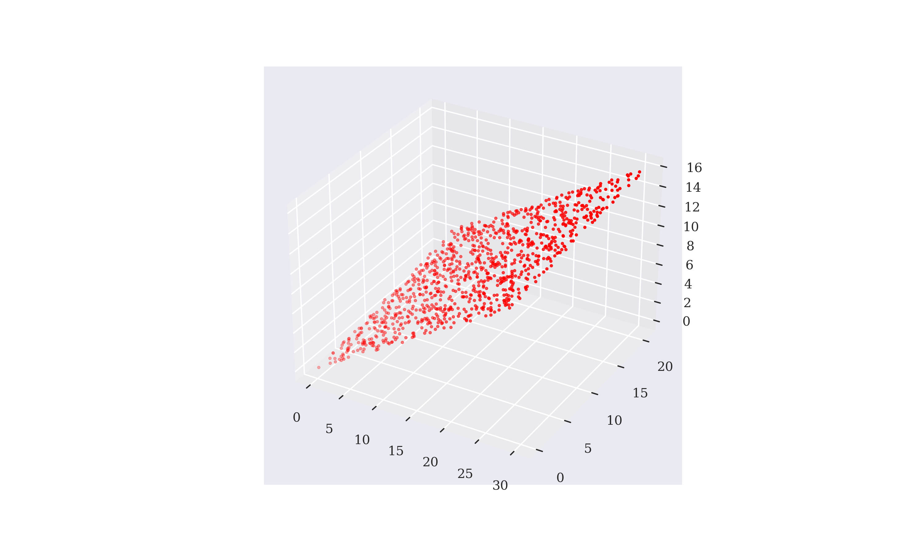
Figure 3-1. Random portfolio payoff vectors visualized in three dimensions

Martingale Pricing

The importance of martingale measures is clear from the First Fundamental Theorem of Asset Pricing (1FTAP) and the Second Fundamental Theorem of Asset Pricing (2FTAP).

In [14]: Q = np.array((0.3, 0.3, 0.4))

In [15]: np.dot(Q, S[1])
Out[15]: 11.0

Super-Replication

Replication is not only important in a pricing context. It is also an approach to hedge risk resulting from an uncertain contingent claim payoff. Consider an arbitrary attainable contingent claim. Selling short the replication portfolio in addition to holding the contingent claim eliminates any kind of risk resulting from uncertainty regarding future payoff. This is because the payoffs of the contingent claim and the replicating portfolio cancel each other out perfectly. Formally, if the portfolio ${\varphi }^{*}$ replicates contingent claim $C_1$, then

For a contingent claim that is not attainable, such a perfect hedge is not available. However, one can always compose a portfolio that super-replicates the payoff of such a contingent claim. A portfolio $\varphi$ super-replicates a contingent claim $C_1$ if its payoff in every future state of the economy is greater or equal to the contingent claims payoff $V_1\left(\varphi \right)\ge C_1$.

Consider again the first Arrow-Debreu security ${\gamma }^u$ which is not attainable. The payoff can be super-replicated, for example, by a portfolio containing the risk-less bond only:

The resulting payoff is

where the $\ge$ sign is to be understood element-wise. Although this satisfies the definition of super-replication, it might not be the best choice in terms of the costs to set up the super-replication portfolio. Therefore, a cost minimization argument is introduced in general.

The super-replication problem for a contingent claim $C_1$ at minimal costs is

or

Such minimization problems can be modeled and solved straightforwardly in Python when using the SciPy package. The following code starts by calculating the costs for the inefficient super-replication portfolio using the bond only. It proceeds by defining a value function for a portfolio. It also illustrates that alternative portfolio compositions can indeed be more cost efficient.

In [16]: C1 = np.array((1, 0, 0))  

In [17]: 1 / B[1][0] * B[1] >= C1  
Out[17]: array([ True,  True,  True])

In [18]: 1 / B[1][0] * B[0]  
Out[18]: 0.9090909090909092

In [19]: def V(phi, t):  
             return phi[0] * B[t] + phi[1] * S[t]

In [20]: phi = np.array((0.04, 0.03))  

In [21]: V(phi, 0)  
Out[21]: 0.7

In [22]: V(phi, 1)  
Out[22]: array([1.04, 0.74, 0.59])

The payoff of the contingent claim (first Arrow-Debreu security).

The portfolio with the bond only checked for the super-replication characteristic.

The costs to set up this portfolio.

A function to calculate the value of a portfolio phi today t=0 or in one year t=1.

Another guess for a super-replicating portfolio.

The cost to set it up which is lower than with the bond only.

And the resulting value (payoff) in one year which super-replicates the first Arrow-Debreu security.

The second part of the code implements the minimization program based on the inequality constraints from above in vectorized fashion. The cost optimal super-replication portfolio is much cheaper than the one using the bond only or the already more efficient portfolio including the bond and the stock.

In [23]: from scipy.optimize import minimize  

In [24]: cons = ({'type': 'ineq', 'fun': lambda phi: V(phi, 1) - C1})  

In [25]: res = minimize(lambda phi: V(phi, 0),  
                        (0.01, 0.01),  
                        method='SLSQP',  
                        constraints=cons)  

In [26]: res  
Out[26]:      fun: 0.3636363636310989
              jac: array([10., 10.])
          message: 'Optimization terminated successfully'
             nfev: 6
              nit: 2
             njev: 2
           status: 0
          success: True
                x: array([-0.0303 ,  0.06667])

In [27]: V(res['x'], 0)  
Out[27]: 0.3636363636310989

In [28]: V(res['x'], 1)  
Out[28]: array([ 1.00000e+00,  3.33333e-01, -4.17100e-12])

Imports the minimize function from scipy.optimize.

Defines the inequality constraints in vectorized fashion based on a lambda (or anonymous) function; the function $\lambda$ modeled here is $\lambda \left(\varphi \right)=V_1\left(\varphi \right)-C_1$ for which the inequality constraint $\lambda \left(\varphi \right)\ge 0$ must hold.

The function to be minimized also as a lambda function.

An initial guess for the optimal solution (not too important here).

The method to be used for the minimization, here Sequential Least Squares Programming (SLSQP).

The constraints for the minimization problem as defined before.

The complete results dictionary from the minimization, with the optimal parameters under x and the minimal function value under fun.

The value of the optimal super-replicating portfolio today.

The future uncertain value of the optimal super-replicating portfolio; the optimal portfolio which sells short the bond and goes long the stock exactly replicates the relevant payoff in two states and only super-replicates in the middle state.

Approximate Replication

Super-replication assumes a somewhat extreme situation: the payoff of the contingent claim to be super-replicated must be reached or exceeded in any given state under any circumstances. Such a situation is seen in practice, for instance, when a life insurance company invests in a way that it can meet under all circumstances — which often translates in the real world into something like “With a probability of 99.9%." — its future liabilities (contingent claims). However, this might not be an economically sensible or even viable option in many cases.

This is where approximation comes into play. The idea is to replicate the payoff of a contingent claim as good as possible given an objective function. The problem then becomes to minimize the replication error given the traded financial assets.

A possible candidate for the objective or error function is the mean squared error (MSE). Let $V_1\left(\varphi \right)$ be the value vector given a replication portfolio $\varphi$. The MSE for a contingent claim $C_1$ given the portfolio $\varphi$ is

This is the quantity to be minimized. For an attainable contingent claim, the MSE is zero. The problem itself in matrix form is

In linear algebra, this is a problem that falls in the category of ordinary least-squares regression (OLS regression) problems. The problem above is the special case of a linear OLS regression problem.

NumPy provides the function np.linalg.lstsq that solves problems of this kind in a standardized and efficient manner.

In [29]: M = np.array((B[1], S[1])).T  

In [30]: M  
Out[30]: array([[11, 20],
                [11, 10],
                [11,  5]])

In [31]: reg = np.linalg.lstsq(M, C1, rcond=-1)  

In [32]: reg
         # (array,   
         #  array,  
         #  int,  
         #  array)  
Out[32]: (array([-0.04545,  0.07143]), array([0.07143]), 2, array([28.93836,
          7.11136]))

In [33]: V(reg[0], 0)  
Out[33]: 0.2597402597402598

In [34]: V(reg[0], 1)  
Out[34]: array([ 0.92857,  0.21429, -0.14286])

In [35]: V(reg[0], 1) - C1  
Out[35]: array([-0.07143,  0.21429, -0.14286])

In [36]: np.mean((V(reg[0], 1) - C1) ** 2)  
Out[36]: 0.02380952380952381

The future price matrix of the two traded financial assets.

This solves the linear OLS problem by minimizing the MSE.

The optimal portfolio positions, that is the solution to the problem.

The MSE obtained from the optimization procedure (minimal mean squared replication error).

Rank of matrix $M$ …

… and its singular values.

The value of the approximate portfolio (lower than the value of the cost-minimizing portfolio).

The payoff of the approximate portfolio.

The vector with the replication errors.

The MSE from the approximate replication.

Approximate replication might not be applicable in all circumstances. But an investor or financial manager with discretion in their decisions can decide that an approximation is simply good enough. Such a decision could be made, for example, in cases in which super-replication might be considered to be too costly.

Capital Market Line

Assume a mean-variance or rather mean-volatility context. In what follows, the risky stock is interpreted as the market portfolio. One can think of the market portfolio in terms of a broad stock index — in the spirit of the S&P 500 stock index.

As before, agents can compose portfolios that consist of the bond and the market portfolio. The rate of return for the bond — the risk-less interest rate — is $i=0.1$, the volatility is 0. The expected rate of return for the market portfolio is

Its volatility is

Quick calculations in Python give the corresponding numerical values.

In [37]: mu_S = 7 / 6 - 1  

In [38]: mu_S  
Out[38]: 0.16666666666666674

In [39]: sigma_S = (S[1] / S[0]).std()  

In [40]: sigma_S  
Out[40]: 0.6236095644623235

The expected return of the market portfolio.

The volatility of the returns of the market portfolio.¹

Feasible mean values for a normalized portfolio with total weight of 1 or 100% consisting of the bond and the market portfolio without short selling range from 0 to about 0.166. Regarding the volatility, values between 0 and about 0.623 are possible.

Allowing for short selling, Figure 3-2 shows the capital market line (CML) resulting from different portfolio compositions. Because short selling of the bond is allowed, risk-return combinations on the upper line (with positive slope) are possible which is what is referred to in general as the CML. The lower line (with negative slope) is in principle irrelevant since such portfolios, resulting from short positions in the market portfolio, have lower expected rates of return at the same risk as those that have a corresponding long position in the market portfolio.

In [41]: s = np.linspace(-2, 2, 25)  

In [42]: b = (1 - s)  

In [43]: i = 0.1  

In [44]: mu = b * i + s * mu_S  

In [45]: sigma = np.abs(s * sigma_S)  

In [46]: plt.figure(figsize=(10, 6))
         plt.plot(sigma, mu)  
         plt.xlabel('$sigma$')
         plt.ylabel('$mu$')
Out[46]: Text(0, 0.5, '$\mu$')

The market portfolio position takes on values between -200% and 200%.

The bond portfolio position fills up to 100% total portfolio weight.

The risk-less interest rate.

The resulting expected rates of return for the portfolio.

The resulting volatility values for the portfolio.

Plots the CML for short as well as long positions in the market portfolio.

Figure 3-2. Capital market line

The equation describing the (upper, increasing part of the) CML is

Capital Asset Pricing Model

The capital asset pricing model (CAPM) as pioneered by Sharpe (1964) is an equilibrium pricing model that mainly relates the expected rate of return of an arbitrary financial asset or portfolio and its volatility with the market portfolio’s expected rate of return and volatility.

To this end, the correlation between the rates of return of a financial asset and the market portfolio is of importance. In addition to the market portfolio consider another risky financial asset with price process $T=(T_0,T_1)$. The correlation $\rho$ is defined by

with $-1\le {\rho }_{ST}\le 1$. If the correlation is positive, the two financial assets have a tendency to move in the same direction. If it is negative, the financial assets have a tendency to move in opposite directions. In the special case of perfect positive correlation ${\rho }_{ST}=1$, the two financial assets move all the time in the same direction. This is true, for instance, for portfolios that lie on the CML for which the rates of return are just the rates of return of the market portfolio scaled by the weight of the market portfolio. Uncertainty in this case arises from the market portfolio part only such that any variation in risk is due to the market portfolio weight variation.

Consider the case of a financial asset $T$ which is part of the market portfolio and for which the correlation with the market portfolio shall not be perfect. For such a financial asset, the expected rate of return is given by:

It is easy to verify that the correlation between the market portfolio and the bond is zero such that the above relationship gives the risk-less interest as the expected return if the financial asset $T$ is the risk-less bond.

The covariance between $S_1$ and $T_1$ is defined as ${\sigma }_{ST}={\rho }_{ST}·{\sigma }_S·{\sigma }_T$ such that

with

This gives the famous CAPM linear relationship between the expected rate of return of the market portfolio and the expected return of the financial asset $T$ — or any other financial asset to this end. In that sense, the CAPM states that the rate of return for any financial asset is only determined by the expected excess return of the market portfolio over the risk-less interest rate and the beta factor which is the covariance between the two, scaled by the square of the market portfolio volatility (variance of returns).

For the CAPM, the CML is replaced by the security market line (SML) which is plotted in beta-return space below. A visualization is given in Figure 3-3.

In [47]: beta = np.linspace(0, 2, 25)  

In [48]: mu = i + beta * (mu_S - i)  

In [49]: plt.figure(figsize=(10, 6))
         plt.plot(beta, mu, label='security market line')  
         plt.xlabel('$\beta$')
         plt.ylabel('$mu$')
         plt.ylim(0, 0.25)  
         plt.plot(1, mu_S, 'ro', label='market portfolio')  
         plt.legend(loc=0);

Generates a ndarray object with the beta values.

Calculates the expected returns mu according to the CAPM.

Plots the beta-mu combinations.

Adjusts the limits for the y axis.

Plots the beta and expected return of the market portfolio.

Figure 3-3. Security market line

But why do the above relationships — and in particular the CAPM formula — hold true in the first place? To answer this question, consider a portfolio with normalized weight of 1 or 100% of which a proportion $a$ is invested in financial asset $T$ and the remainder $1-a$ is invested in the market portfolio. The expected rate of return of this portfolio is:

The volatility of the portfolio is (see Sharpe (1964)):

The marginal change in the expected portfolio rate of return, given a marginal change in the allocation of the financial asset $T$, is determined by the following partial derivative:

The marginal change in the portfolio volatility, given a marginal change in the allocation of the financial asset $T$, is determined by the following partial derivative:

The basic insight of the CAPM as an equilibrium model is that the financial asset $T$ is already part of the market portfolio. Therefore, $a$ can only be interpreted as the excess demand for the financial asset and in equilibrium when excess demand for all financial assets is zero, $a$ also must equal zero. Therefore, in equilibrium, the partial derivative for the expected portfolio rate of return remains unchanged while the one for the portfolio volatility simplifies significantly when evaluated at the equilibrium point $a=0$.

The risk-return trade-off in market equilibrium therefore is:

The final insight needed to derive the CAPM formula from above is that in equilibrium the above term needs to be equal to the slope of the CML:

How does the CAPM help in pricing a financial asset that is not replicable? Given the vector of uncertain prices in one year of a financial asset $T_1$ the uncertain rates of return are

where $T_0$ is the equilibrium price today to be determined. The following relationship holds as well

Define now the unit price of risk as the excess return of the market portfolio per unit of variance by

such that according to the CAPM one gets:

This shows that in equilibrium the expected rate of return of a financial asset is determined only by its covariance with the market portfolio. Equating this with the above term for the expected return of the financial asset $T$ yields

The denominator can be thought of as a risk-adjusted discount factor.

Conclusions

The major topic of this chapter is incomplete financial markets. Moving from a two state model economy to one with three states and keeping the number of traded financial assets constant at two, market incompleteness is an immediate consequence. This in turn implies that contingent claims are in general not perfectly replicable by portfolios composed of the risk-less bond and the risky stock.

However, payoffs of contingent claims can be super-replicated if they must be met or surpassed under all circumstances. While there are in general infinitely many such super-replication portfolios, it is in general required that the cost minimal portfolio be chosen. If there is a bit more flexibility, the payoffs of contingent claims that are not attainable can also be approximated. In this context, the replication problem is replaced by an optimization problem according to which the mean squared error of the replication portfolio is minimized. Mathematically, this boils down to a linear ordinary least-squares regression problem.

The Capital Asset Pricing Model is based on equilibrium pricing arguments to derive expected rates of return and also prices for traded financial assets given their risk-return characteristics in the mean-volatility space. A central role is played by the correlation and the covariance of a financial asset with the market portfolio which is assumed to contain the financial asset itself.

Further Resources

Papers cited in this chapter:

• Sharpe, William (1964): “Capital Asset Prices: A Theory of Market Equilibrium under Conditions of Risk.” The Journal of Finance, Vol. 19, No. 3, 425-442.

Books cited in this chapter:

• Pliska, Stanley (1997): Introduction to Mathematical Finance. Blackwell Publishers, Malden and Oxford.