13
Smart Surveillance Video Stream Processing at the Edge for Real‐Time Human Objects Tracking
Seyed Yahya Nikouei Ronghua Xu and Yu Chen
13.1 Introduction
The past decade has witnessed worldwide urbanization because of the benefits and diverse lifestyles in bigger cities. While it brings higher living quality, it introduces new challenges to city administrators, urban planners, and policy makers. Safety and security are among the top concerns when more and more people live in an area with such a high density. Situational awareness (SAW) has been recognized as one of the key capabilities in order to timely deal with urgent issues. To serve this purpose, more and more surveillance cameras and sensors are installed in urban area to monitor the daily activities of the residents. For example, North America alone had more than 62 million cameras by 2016 [1]. The enormous surveillance data generated by these cameras requires extraordinary supervisory action to extract useful information, which implies 24/7 attention to the captured video streams. It is not realistic to rely on human operators facing the ubiquitously deployed cameras. Recent machine‐learning algorithms are promising to make smarter decisions based on surveillance video in real time. However, intelligent decision‐making approaches is not mature yet today.
When each frame is taken, it must be transferred from the field to the data center where further processing. Nowadays, the video data dominate the real‐time traffic and creates heavy workload on the communication networks. Online video streaming accounts for 74% of the online traffic in 2017 [2], and 78% of mobile traffic will be video data by 2021 [3]. A single camera generates more than 9600 GB of data in a single day. There are a couple of important concerns the community is aware of and has been working hard to resolve. First of all, it is essential to avoid sending raw data that is not globally significant to reduce the heavy burden on the communication network. Also, the transmission time for the raw footage to reach the data center can be vital in some delay‐sensitive, mission‐critical applications. It is desired to reduce the communication delays as much as possible. Second, one of the important issues is data loss during transmission, or even worse, that a third‐party eavesdrops on the transmission line. Considering the huge volume of video data to be stored in the data center, new challenges are introduced. While the capacity of data storage facilities is getting larger and larger, nowadays the surveillance video owners can merely keep weeks of the most recently captured footages. The limited storage capacity results in losing footage that contains important information for forensics analysis or other purposes. Thus, it is critical to be able to timely extract features from raw video such that the operators can identify and selectively store the clips of interest for longer periods.
In order to address these problems, edge and fog computing and distributed real‐time data processing are attracting a lot of attention in the surveillance community [5]. The functions, including feature extraction and decision making, are migrated to the edge of the network, and a distributed environment is created instead of a single or couple points of reference. In this chapter, an edge computing based smart surveillance system is introduced [6]. Focusing on human object detection, the system takes three steps toward an intelligent decision‐making. First, it recognizes and detects human objects in each given frame and each human object is tracked for feature extraction. The speed or movement direction of each human object is saved in an array along with other specific information as features for next step. The final step enables decision‐making using machine‐learning algorithms based on time‐series features, which decides whether an alarm should be generated to the higher levels or human operators in charge. Figure 13.1 shows the network architecture and tasks allocated in each layer. In this figure, human detection and tracking are considered to be accomplished at the edge of the network and more computing intensive decision‐making algorithms will take place at the fog level where tablets or notebooks are available, and then in final decision in case of an incident is sent to the person in charge or first responders.

Figure 13.1 Edge‐fog‐cloud‐based hierarchy smart surveillance architecture.
In this chapter, the computations and algorithms used at the edge and fog levels are discussed and compared to create such automated surveillance system. The rest of this chapter is organized as the follows. Section briefly introduces the human object identification algorithms that are potentially feasible in the edge computing environment, followed by the object tracking algorithms in the Section . Section is focused on the design issues of a lightweight human object detection scheme and a case study using Raspberry Pi as the edge device is presented in Section . At the end, Section summarizes this chapter with some discussions.
13.2 Human Object Detection
Although there are many publications devoted to human detection in general [4, 7], this task has not been thoroughly investigated on the devices with limited computing resources, such as the ones at the edge of the network. Human detection can be done using different accepts and algorithms. This chapter highlights three of them, which are potentially able to be fit into the edge computing environments.
13.2.1 Haar Cascaded‐Feature Extraction
Haar cascaded‐feature extraction is a well‐studied method for human face or eye detection with decent performance [8]. It can also be applied for full human body detection. The algorithm subtracts pixel values from each other based on Haar‐like features. There are a huge number of ways pixel values can be picked and subtracted, such that the learning process is normally conducted on a very powerful CPU. With a 24 × 24 image, about 160,000 features are produced. After training the algorithm is fast because only some subtractions need to take place.
Figure 13.2 shows several typical Haar‐like features. There are three types of features, including two rectangular features (Figure 13.2 (a)), three rectangular features (Figure 13.2 (b)), and four rectangular features (Figure 13.2 (c)). In each feature, the pixel values in the black area are subtracted from the pixel values in the white area. In the learning phase, around 2000 positive images (containing the object of interest) and about half this size negative images are selected. These feature sets convolute over the image and a vector of values is created. Then an algorithm by the name of Adaboost will pick the best‐performing features for the detection and thresholds found. Thus, the existence of the object in the image is determined by applying the selected features and a matching score above the thresholds.
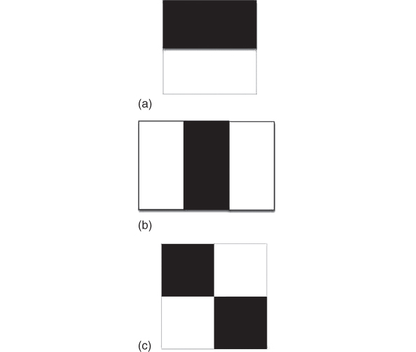
Figure 13.2 Haar‐like features: (a) two rectangular features; (b) three rectangular features; (c) four rectangular features.
However, in terms of speed the performance is far from satisfactory because of the huge number of features used for higher accuracy. Therefore, a hierarchy method is introduced. It screens the input image by running the most important features first. If the result is positive, implying there might be an object of interest in the frame, more features will be tested. For instance, in first step, only one of the most dominating features is applied. A negative result means that the chance of existence of the object of interest in the frame is very low. Otherwise, a positive result leads to further tests with more features for fine position tuning and higher accuracy. In one example reported in literature, there are 28 stages in total, where the first stage has 1 feature, the second stage has 10 features, and the third stage has 25 features [9].
13.2.2 HOG+SVM
HOG+SVM is another widely used method because of its high accuracy. The name comes from a feature extraction named histogram of oriented gradients (HOG) and support vector machine (SVM) [11, 12]. These features are applied to classify or detect objects of interest. Traditionally, the high computing cost of this feature extractor makes the overall object detector not an ideal candidate for the edge computing environments. However, with more powerful devices deployed at the edge, the HOG+SVM method becomes more attractive for its accuracy. No matter how complicated or simplified a classifier is, if the features used for classification do not describe the object of interest in the best way the detection result will be inaccurate. For example, when oranges are to be separated from apples, while the orange color of the fruit is a good feature, the sphere shape does not give useful information for classification.
HOG is a well‐known method for feature extraction. The difference in vertical neighboring pixels to the target pixel are considered as the vertical differential and the same method is also used to calculate the horizontal differential. It is worth mentioning that in some cases, instead of using only two immediate neighbors a vector of several pixels in each direction can be used, which contains more information for each pixel. The horizontal and vertical values are considered as an amplitude and angle instead of two derivatives. The horizontal derivative fires on vertical lines and the vertical derivative fires on horizontal lines. If there is more than one input channel such as RGB images with three channels, then the highest amplitude, along with its corresponding angle, are chosen to represent a pixel's gradient.
A histogram with nine bins is usually used with 0–20 degrees in each bin to represent the unsigned gradients and the amplitude of the respective angle is considered in the corresponding bin. If, however, the angle is closer to the border of a bin, part of the amplitude is given to the neighboring bin. The histogram is created for a window of 8×8 pixels normally. In order to resolve the effect of lightning or other temporary changes related to pixel values, normalization is needed [10]. In most object detection cases, 32×32 windows are selected to reduce processing time. This bigger window strides through the image with step of 1, which means a 4×4 of batches of windows of size 8×8 pixels is selected and then one 8×8 goes out from the 32×32 window from left and another one enters from the right. Each 32×32 window has 16 histogram bins in it, which can be represented in a 144 vector. The vector is normalized with the second norm of the vector values. Each vector is used as features for a part of image for object detection in the SVM. Figure 13.3(a) shows one of these before normalized histogram for an 8×8 super pixel and Figure 13.3(b) represents the gradient calculations in a 64×64 window (window is bigger than 8×8 pixels because of better visibility).

Figure 13.3 (a) Histogram of oriented gradients; (b) representation of HOG on an image.
Another problem arises when human objects are closer or farther away from the camera in different camera placements. Taking a fixed window such as 8×8 is not useful if the person is very close or 16×16 might be too big when human objects are far away. An image pyramid is implemented in this case to change the resolution of the image and detect every possible object. Each stage reduces the pixels to create smaller image versions so that a super pixel covers bigger portions of the image. Consider that multiple stages of the image may result in multiple positive outputs for the same object. Figure 13.4 illustrates such a scenario. It is needed to change the variables in every specific usage to guarantee the best results, which means the algorithm is not good for generalization.

Figure 13.4 An example of multi‐detection for a single object.
13.2.3 Convolutional Neural Networks (CNNs)
Convolutional neural networks (CNNs) are based on multi‐layer perceptron (MLP) network, one of the most famous types of neural networks, which have convolutional layers to produce feature maps.
CNNs usually have two separable parts, one is the convolutional layers and the other is a fully connected neural networks (FCNNs) or in some cases SVM classifier, which classifies objects using the feature map created by the convolutional layers. In each convolutional layer, a set of filters convolute with the input and the dot product will be reconsidered as the output. After a convolutional layer, which is considered as a linear layer, a ReLU layer is added so that nonlinearity is introduced to the network. To keep the dimensionality unchanged, a padding of pixels around the input with a value of zero is added. Spatially downsizing of the feature map will be done with the pooling layers, where in a 2×2 square of values, the highest one is selected or the average value is calculated. At the final convolutional layer, only a series will be remained from the input image and that is used for classification.
Image classification generally refers to the process of giving the computer one image and the computer outputs a label about the most dominant object in the image which the image is taken from. In 2012, Alexander Krizhevsky's network showed very promising results for image classification [13]. The architecture is commonly known as AlexNet and it won the most accurate network in the ImageNet contest. In the following year, VGG [14] was introduced. This network had the same structure as the AlexNet with some little changes in the filter size and layer number. VGG was the winner of 2013. In order to compete in ImageNet, the architectures need to classify 1000 objects and so the training needs 1000–1500 images from each class, and ImageNet provides this vast labeled dataset for public use.
In 2014, Google released another architecture GoogleNet that won the best accuracy in ImageNet [15]. The architecture of GoogleNet is different from the previous models. Although it still consists of convolutional layers and fully connected network at the end, GoogleNet adopts inception modules, which are some convolutional layers executing in parallel, and then they connect to a layer's input. In 2015, ResNet [16] was released by Microsoft, and to date, many modified architectures based on the residual blocks of ResNet have been introduced. This module has outputs not only to the immediate higher level convolutions but also to layers higher than the immediate layer.
The filter size and network architecture are predefined. During the training phase, the filter values that are generated randomly are tuned for best performance. Also, the weights of the classifier at the end of the network are based on the training phase. After that, the network is relatively fast. Training is usually based on back propagation algorithm and takes about 100,000 epochs to complete, where each round through all training image sets is defined one epoch.
There are models that are specifically designed for working with CNNs. Caffe model [20] from the University of Berkley is a well‐known framework. This model is considered a low‐level architecture. The main advantage lies in the fast training and implementation. Meanwhile, the main disadvantage of Caffe model is that it does not have unified and complete documentation, and this may confuse a beginner.
Another widely used framework is TensorFlow from Google [21]. This model works well in a parallel GPU environment and is used as a back engine for other higher‐level models such as Keras [22]. A lighter version of this model is introduced for fog level or some powerful edge devices last year. OpenCV 3.3 also has libraries necessary to load and do forward propagation on architectures created by Caffe or Tensorflow. Keras was created to make designing, training, and testing CNNs easier. It has a high‐level approach accessible through Python. The model then transforms the code into TensorFlow and does the training or forward propagation. Many of the confusing details of low‐level models are not accessible with Keras, but it is convenient to work with. The models in Caffe are in a simple text, and for a big architecture it is hard to handle the code. However, in Keras it is very compressed and also in Python, which is easier to manage. MxNet is another high‐level model Python, which is also very good for parallelism.
In smart surveillance system, the camera needs to give the location of the detected object. Thus, image classification might not be helpful, as there might be several people in one given frame and classifying the image as containing humans does not contribute value in this category. In this context, object detection is required, where the detector gives the bounding box around the object of interest with a label of the detection. Single Shot Multi‐box Detector (SSD) [17] or Regional CNN (R‐CNN) [18, 19], along with other models, are introduced to create a prediction not for the whole image but for neighborhood where the object is located. Training an architecture of this kind needs images from the object that are labeled and also the object is marked within the image. In SSD structure, based on the features that are extracted from the source image, the network makes predictions of the objects that might exist in a certain region.
Although the performance of the neural networks is decent at the edge device and more recent architectures such as GoogleNet have very accurate rates, these models need a huge volume of RAM space, which might not be available in a resource‐limited device. For example, when loading the VGG network on the selected edge device (Raspberry Pi), the model gave an error because the available RAM space is low and the program was interrupted. Therefore, more compact architectures to be used at the network edge is expected.
13.3 Object Tracking
Object tracking plays an important role in human behavior analysis in smart surveillance systems. The main purpose of tracking algorithms is to generate the trajectory of the object over time by calculating its position in every frame of the video stream. Compared to object detection that is responsible for isolating a specific region of frame and identifying target object, object tracking is focused on establishing correspondence between the object instances across frames [25]. In object tracking approaches, the detection and tracking can work either separately or jointly to generate trajectory of object. In the first case, object detection algorithm extracts a region of interest (ROI) from every frame. Then the tracking algorithm corresponds object instances across frames by means of marked object regions. In the latter case, object detection and tracking work jointly as one algorithm to compute trajectory of objects by iteratively updating object features obtained from previous frames. Challenges in object tracking are summarized as follows [27]:
- Loss of evidence caused by estimating the 3D realm on a 2D image
- Noise in an image
- Difficult object motion
- Imperfect and entire object occlusions
- Complex objects structures
Those challenges are mainly associated with object feature representation. The following subsections discuss feature representations and classifications of object tracking methods according to selected object features.
13.3.1 Feature Representation
Selecting the accurate feature representation is important to object tracking. Identified objects by means of object detection algorithms are represented as either shape model or appearance model. Whether it is the shape or appearance model, feature selection strictly depends on which characteristics will be used for describing object model. The object can be described using color, edge, and texture.
- Color. Each frame of video is an image that is represented by using certain type of color space models ranging from gray scale, RGB, YCbCr, and HSV. In each image, the data are stored as a layered matrix in which value in each cell is brightness of spectral band. For example, colorful images are denoted as a three‐layered matrix that consists of red (R), green (G), and blue (B), while gray images decompose color into one channel‐gray value. HSV or HLS decompose colors into their hue (H), saturation (S), and value/luminance (V) components.
- Edge. Edges are regions in the image with large variation in intensity in opposite directions. Edge‐detection algorithms take advantage of variation in intensity to find edge regions, then draw contour of object through connecting edges. The most significant property of edges is that they are less sensitive to illumination changes compare to color features. However, demarcation boundaries between different objects are difficult, especially when multiple objects are overlapped. Edge detection is a fundamental method in image processing, especially in feature detection and feature extraction.
- Texture. Texture is a degree of intensity dissimilarity of a surface that enumerates properties such as smoothness and regularity. Image texture usually includes information about the spatial arrangement of color or intensities in an image or selected region, which could be useful features for object detection and tracking. Compared to color space model, texture obeys statistical properties and has similar structures. It requires an analytical processing step to calculate features. Texture analysis approaches are structural approach, statistical approach, and Fourier approach. Like edge features, the texture features are less sensitive to illumination changes than color space in image.
The model of representing object limits the type of features that can be leveraged in tracking algorithms, such as motion and deformation. For example, if an object is represented as a point, then only a translational model can be used; when a geometric shape representation such as an ellipse is used for representing the object, parametric motion models like affine or projective transformations are appropriate [26].
13.3.2 Categories of Object Tracking Technologies
Figure 13.5 shows a taxonomy of tracking approaches. In general, object tracking technologies can be categorized into three groups: point‐based tracking, kernel‐based tracking, and silhouette‐based tracking [27].

Figure 13.5 Object tracking methods.
The following subsections offer a detailed discussion in those tracking approaches by illustrating the underlying algorithms and analyzing their characteristics.
13.3.3 Point‐Based Tracking
Point‐based tracking can be formulated as the correspondence of detected objects represented by points across frames [25]. In general, point‐based tracking can be divided into two board categories according to the point correspondence methods: deterministic methods and statistical methods. The deterministic approaches exploit qualitative motion heuristics to solve the correspondence problem, and the statistical methods use probabilistic models to establish correspondence. Several widely applied methods such as Kalman filter, particle filter, and multiple hypotheses belong to the statistical category.
13.3.3.1 Deterministic Methods
Deterministic methods are essentially formulated as the combinatorial optimization problem that attempts to minimize the correspondence cost. The correspondence cost is usually defined by a combination of different motion constraints [27], which are shown in Figure 13.6.

Figure 13.6 Different motion constrains.
- Proximity assumes the position of object would not change significantly from previous frame to current frame (Figure 13.6 (a)).
- Extreme velocity defines the upper bound of object's position and limits the possible correspondence to the neighborhood around the object in a circular region (Figure 13.6 (b)).
- Minor velocity (smooth motion) assumes both direction and speed of the object should not change notably (Figure 13.6 (c)).
- Common velocity (smooth motion) assumes objects in a small neighborhood should have similar direction and velocity between frames (Figure 13.6 (d)).
All of the above constraints are not specific to the deterministic methods only. They can also be used in statistical methods for point tracking. Deterministic methods are appropriate in object tracking tasks in which objects are usually very small compared with surrounding context.
13.3.3.2 Kalman Filters
A Kalman filter [28], also known as a linear quadratic estimation (LQE), is based on Optimal Recursive Data Processing Algorithm. Using a series of measurements observed over time, a Kalman filter could produce estimates of unknown variables based on recursive computational means. A Kalman filter is appropriate to estimate the optimal state of a linear system where the state and noise have a Gaussian distribution. Kalman filters work in a two‐step process: prediction and correction. The prediction process predicts the new state of the variables given a current set of observations. The correction step gradually updates the predicted values and generates the optimal approximation of the next state [27].
13.3.3.3 Particle Filters
In cases where the object state is not assumed to be a Gaussian distribution, Kalman filter will give poor estimations of state variables due to the limitation of requiring the state variables to be normally distributed (Gaussian). In such situations, particle filters [29] is better to perform state estimation. A particle filter generates all models for one variable before processing the next variable. It calculates the conditional state density at time t to represent the posterior distribution of stochastic process by using a genetic mutation‐selection sampling approach with a set of particles. The particle filter is actual a Bayesian sequential importance technique, which recursively approaches the later distribution using a finite set of weighted trials [27]. Contours, color, and texture are all features used in a particle filter algorithm. Like Kalman filters, particle filters also consist of two basic steps: prediction and correction.
13.3.3.4 Multiple Hypothesis Tracking (MHT)
If only two frames are used in motion correspondence processes, there is a limited chance of a correct correspondence. To get better tracking results, correspondence decisions could be performed when several frames have been evaluated. Thus, multiple hypothesis tracking (MHT) algorithms maintain multiple correspondence estimates for each object at each frame. The final object track is the trajectory, including the entire set of correspondences during the time periods of observation. MHT is an iterative algorithm. An iteration starts by feeding a set of current track hypotheses, and each hypothesis is a collection of mutual independent tracks [25]. Through establishing correspondence for each hypothesis based on the distance measurement, a new hypothesis that represents a new set of tracks is generated as the result of prediction process. MHT is good at tracking multiple objects, especially in those scenarios where objects enter and exit the field of view (FOV).
13.3.4 Kernel‐Based Tracking
Kernel‐based tracking methods compute motion of kernel on each frame to estimate movement of the object. In kernel‐based tracking, kernel refers to the object representations in the form of a rectangular or ellipsoidal shape and object appearance. Kernel‐based tracking algorithms are divided into four categories: template matching, mean‐shift method, support vector machine (SVM), and layering‐based tracking.
In template‐matching tacking, a set of object template O t is defined in the previous frame, and tracking algorithms use a brute force method to search a region that is most similar to the predefined object template. The position of possible templates in the current frame is produced after the similarity measurement. Since templates are generated by means of image intensity or color features, which is sensitive to illumination changes, template‐matching algorithms are preferable to detect small pieces of a reference image. The brute force searching in measuring template similarity leads to a high computation cost. Therefore, the template‐matching tracking is not suitable for multiple‐object tracking scenarios in a device with limited resources.
Instead of using the brute force method, mean‐shift–based algorithm takes advantage of mean‐shift clustering [30] technology to detect the region of object that is most similar to a reference model. By comparing the histograms of the object and the window around the hypothesized object location, the mean‐shift tracking algorithm attempts to maximize the appearance similarity iteratively. It usually takes five to six iterations until convergence is achieved; thus, mean‐shift tracking requires less computational cost than template‐matching tacking does. However, mean‐shift tracking assumes that a portion of the object is inside the circular region in initial state. Physical initialization is necessary during initialization of the tracking task. Additionally, mean‐shift algorithm is only capable of tracking one single object.
Avidan first integrated the SVM classifier into an optic‐flow‐based tracker [31]. Given a set of positive and negative training samples, SVM is preferable to handle binary classification problems through finding the best separating hyperplanes between two classes. In SVM‐based tracking, tracked objects are labeled as positive, while untracked objects are defined as negative. The tracker could use trained SVM classifiers to estimate the position of the object by maximizing the SVM classification score over an image's region. SVM‐based tracking can handle partial occlusion of the tracking object. However, it needs training process to prepare the SVM classifier before performing the tracking task.
In layering‐based tracking, each frame is separated into three layers: namely, shape representation (ellipse), motion (such as translation and rotation), and layer appearance (based on intensity) [32]. In layering‐based tracking, at first, layering is achieved by compensating the background motion, then object position is estimated by calculating a pixel's probability based on the object's foregoing motion and shape features. Layering‐based method is appropriate in scenarios where multiple objects are tracked or fully occlusion of objects happens.
13.3.5 Silhouette‐Based Tracking
For objects with complex shapes, which are difficult to be well described by simply using geometric features, for example, hands, head, and shoulders, silhouette‐based algorithm provides a better solution. According to the object model, silhouette‐based tracking approaches are categorized as either contour tracking or shape matching. In contour tracking, initial contour evolves to its new position in the current frame to keep track with the object. In contrast, shape matching only searches object in one frame from time to time by using density functions, silhouette boundary and object edges [32].
The above discussion provides a comprehensive summary of research in object tracking algorithms. In the next section, a detail illustration of the Kernelized Correlation Filter (KCF) tracking method is presented, which achieves good performance in terms of resource consumption.
13.3.6 Kernelized Correlation Filters (KCF)
Tracking‐learning‐detection (TLD) framework is widely used in modern object tracking arts of field [33]. Boosting [34] and multiple instance learning (MIL) [35] demonstrate capability in online training that makes the classifier adaptive while tracking the object. However, updating process consumes a lot of resources. The lower resource consumption with high tracking success rate makes Kernelized Correlation Filter (KCF) a preferable online tracking method in delay sensitive surveillance system.
KCF is initially inspired by successful applications of the correlation filter in tracking [36]. Compared with other complicated approaches, correlation filters have been proved to be competitive in environments with tight constraints on computational power. Object detection using KCF could be defined as a deterministic problem based on Kernel Ridge Regression [37]. The KCF algorithm is essentially a kernelized version of linear correlation filter. Exploiting powerful kernel trick allows transferring unstructured linear correlation filter to linear space, so that KCF has the same computational complexity as linear correlation filter when handles nonlinear regression problem with multiple channel features.
To determine object position in the current frame, template matching is first performed by computing a correlation with a special filter h, and subsequently searches the maximum value on the obtained correlated image c [38]:
- c: Correlated image
- s: Image region for searching
- h: Filter generated from the object template
- °: Operator to calculate two‐dimensional correlation
- (x,y)*: The target object position corresponding to the maximum of correlated image c
Equation 13.1 assumes that the tracking area f and the filter h have the same dimension. The correlated filter h is calculated by the Ridge regression to minimize the squired error over a template t. It is:

- λ: regularization parameter, as in the SVM
- f(x i )=t i ∘h i : Correlation function between template and filter images
- c: Channels of the two‐dimensional images
- g: Two‐dimensional Gaussian distribution function, g(u,v) = exp[–(u 2 + v 2)/2σ 2]
The purpose of the optimization problem defined in Eq. is to find a function h that correlates with object template t to output the minimum difference from Gaussian distribution function g. It is straightforward to work in the frequency domain, where Equation could also be directly transformed into Fourier expression:
- X*: Complex‐conjugation operation of X
- ⊙: Element‐wise product operator
- H: Filter in Fourier domain
- T: Object template in Fourier domain
- G: Gaussian function in Fourier domain
Given the filter H, and the search region F in the frequency domain, combining Equations 13.1 and , correlation image C can be calculated in Fourier domain as:
Finally, given Equations 13.1 and 13.4, the object tracking algorithm is:
where ![]() denotes the inverse DFT operation.
denotes the inverse DFT operation.
In KCF tracking algorithm, in order to increase the object tracking area, the template t is selected as a region with a size larger than the object size. For best results of the KCF tracking method, the template size is suggested to select as 2.5 times larger than the object size [36]. KCF takes advantage of the HOG feature to track objects given the assumption that objects have similar contour even though they have different appearance. Figure 13.7 shows the KCF object tracking process.

Figure 13.7 KCF tracking process.
Detailed illustrations of the feature extraction and object tracking steps are listed as follows:
- Gradient computing. Normalizing the color and gamma values is the first step to calculating the feature detector, which is followed by the calculation of the magnitude and orientation of the gradient.
- Weighted vote in orientation cell. The image is divided based on a sliding detection window and the cell histograms are created. Each pixel within the cell is associated with a weighted vote for an orientation‐based histogram channel according to the values calculated in the previous step of gradient computation.
- Contrast normalization. Considering the effect caused by illumination and contrast change, gradient strengths are locally normalized by grouping the overlapping cells together into larger, spatially connected blocks.
- HOG collection. In this step, the concatenated vector of the components of the normalized cell histograms from all block regions is calculated to create a HOG descriptor.
- KCF tracker. HOG descriptor that contains extracted HOG feature vectors is fed to a KCF tracker for producing hypothesis of target position.
13.4 Lightweight Human Detection
Due to the constraints on resources, lightweight algorithms are required for the edge devices. Normally there are trade‐offs to be considered carefully when designing a light version of an existing algorithm, which often means sacrificing the accuracy or speed. There are two important components to building a good object detector: the feature extractor and the classifier. Considering the algorithms discussed here, classifiers are the most resource‐consuming part of the algorithm, but there are not many changes that can be made to the architecture of these SVMs and FCNNs. Meanwhile, feature extraction algorithms have a lot of room for improvement. Especially in the system that is focused on human objects detection and extracting them from the surrounding environment. Hence, the extracted features are applied as the given input data to make the distinction more noticeable to the classifier.
Haar cascade algorithm is a fast algorithm and it does not map the pixel values to another space for feature extraction. In addition, this algorithm only uses simple mathematical functions such as dot product that are very fast. Therefore, this algorithm is suitable for mobile and edge devices. But its accuracy is not satisfactory.
The HOG algorithm may follow the same principle. However, the video frame can be resized before passing to algorithm. Also, there are many parameters in the algorithm that can be tuned to improve the accuracy. For example, the window that takes pixels for histograms creation can be bigger, which makes the algorithm faster but there is a bigger chance that a pedestrian is ignored. Smaller window sizes make the algorithm run very slowly but most of pedestrians are detected and the chance of having multi‐bounding box for a human object increases. A set of variables for one camera positioning that can be accurate may not perform best for another video; this creates a need to fine tune the algorithm for every camera.
CNN is the focus of attention for simplifications that fit the algorithm on smaller devices. Several architectures are introduced that enable the creation of a more condenses CNN. Some of them are mathematically proven to be able to reduce computational burden. One of these architectures is the Fire module used in SqueezeNet [22]. This architecture has 50 times fewer parameters and has the same performance accuracy as AlexNet. The Fire module has two sets of filters. The first is a convolutional layer with a 1×1 convolution filter. Although it might sound like there is nothing happening in a 1×1 filter, it is reminded that number of channels can be changed. This layer is referred as squeeze layer. Another one is a convolutional layer by the name of expand that consists of a 1×1 set and a 3×3 set of convolutional filters.
MobileNet, which is introduced by Google in 2017 [23], achieves a very good performance and also has less computational burden through a separable depthwise convolutional layer [24]. Where each conventional convolutional layer is split into two parts. A conventional convolution takes F with size D f × D f × M from the input and with filter K of size D k × D k × M × N maps it to G as an output of size D g × D g × N .
The computing complexity of this operation is as Eq. 13.6, and it can be taken into two parts. The first is a depthwise convolutional layer with size
D
k
× D
k
× 1 × M
that can create a ![]() with size
D
g
× D
g
× M
. Then, a set of N pointwise convolutional filters with size of 1 × 1 × M
will create the same G as before. This time the computational complexity becomes as Eq. 13.7.
with size
D
g
× D
g
× M
. Then, a set of N pointwise convolutional filters with size of 1 × 1 × M
will create the same G as before. This time the computational complexity becomes as Eq. 13.7.
This shows a reduction of computational burden by a factor of ![]() as shown in Eq. 13.8.
as shown in Eq. 13.8.

Figure 13.8 compares the network with a separable depthwise convolutional layers and the conventional layers, where the depthwise and pointwise steps are together in a single filter shape. The left‐side is the separable structure and after each depthwise or pointwise convolution, a batch normalization (to normalize the data because one‐time normalization in deep learning is not sufficient) and a ReLU layer are placed.

Figure 13.8 Convolutional filter vs. separable depthwise convolutional filter.
13.5 Case Study
The case study in this section provides more information about the algorithms discussed in this chapter. Implemented on physical edge devices, these algorithms are applied to process sample surveillance video streams.
The selected edge computing device is a Raspberry PI 3 Model B with a 1.2GHz 64‐bit quad‐core ARMv8 CPU and 1GB LPDDR2‐900 SDRAM. The operating system is Raspbian based on the Linux kernel. The fog computing layer functions are implemented on a laptop with a 2.3 GHz Intel Core i7, the RAM memory is 16 GB, and the operating system is Ubuntu 16.04. The software applied for human objects detection and tracking is implemented using C++ and Python programming languages and OpenCV library (version3.3.0) [39].
13.5.1 Human Object Detection
Haar cascades algorithms are very powerful for recognizing individual objects in training data set but not very good with changes. If the positioning or angle of human object does not match the training samples, the algorithm often fails to recognize it. In real‐world surveillance systems, there is no guarantee to always capture pedestrians from the same angles. Figure 13.9 shows a sample video and false positive detections the algorithm generates. In average 26.3% of detections are false in this sample surveillance video, this number may be different in different videos and initial variables. In terms of speed, the performance of this algorithm is very fast at the edge with around 1.82 frames per second (FPS). Considering the velocity of pedestrians, it is sufficient to sample twice per second. From the perspective of resource utility, in average it uses 76.9% of CPU and 111.6 MB of RAM.

Figure 13.9 Results of Haar cascaded human detection.
In contrast, HOG+SVM algorithm on average uses 93% of the CPU, which is expensive because resources are needed by other operations and functions to achieve the goal of a smart surveillance system and 139 MB of RAM. Note that the HOG+SVM algorithm is very slow, 0.304 FPS is reached. Figure 13.10 shows different instances of the sample video in which the bounding boxes are generated by this algorithm. Some of the boxes are not exactly fitted around the human object. For example, in the bottom left screenshot parts of the vehicle is also in the bounding box, which will bring negative impact to the performance of tracking algorithms.

Figure 13.10 Performance of HOG+SVM algorithm.
Based on the approach explained earlier, a lightweight version of CNNs are created. A typical CNN recognizes up to 1000 different classes of objects and the network is too big to be fit in edge devices. Even using MobileNet or SqueezeNet or other examples of such CNNs can take up to 500 megabytes of RAM. For object detection VOC07 is frequently used and it has 21 classes.
However, the major object of smart surveillance systems is to detect human objects, which means there is only one class such that it is not necessary to keep many filters in each layer of the network. Based on this observation, a lightweight CNN network was trained to have four times fewer parameters in each convolutional layer than the MobileNet does. Figure 13.11 shows the results on a Raspberry PI 3 model B. The lightweight CNN takes less than 170 MB of RAM and is relatively accurate and can detect human objects in different angles.

Figure 13.11 Example of light version CNN for human object detection.
13.5.2 Object Tracking
To test feasibility of tracking objects by processing video streams on edge computing devices, a concept‐proof prototype of the system was built using the KCF‐based object tracking algorithm. Here, the performance of the algorithm is presented on object tracking and multi‐tracker lifetime handle such as phase in & out of frame, retracking after tracked object lost, etc.
13.5.2.1 Multi‐Object Tracking
Figure 13.12 shows an example of the multi‐object tracking results. Multi‐tracker object queue is designed to manage tracker lifetime. After the object detection processing finished, all detected objects are fed to the tracker filter, which compares detected target region and the multitracker object queue to rule out the duplicated trackers. Only those newly detected objects are initialized as KCF trackers and appended to the multitracker object queue. During execution time, each tracker runs KCF tracking algorithm independently on target region through processing the video stream frame by frame until the object phases out or it loses the object in the scenario.

Figure 13.12 An example of multi‐object tracking.
13.5.2.2 Object Tracking Phase In and Out
The boundary region is defined to address scenarios when the moving objects enter or exit the current view of frame. In object tracker phase in cases, as objects entered the boundary region, they are detected as new tracking targets with active status and appended to the multi‐tracker queue. In object tracker phase out scenarios, those tracked objects that are moving out of the boundary region will be deleted and the corresponding trackers transfer to inactive status. After a frame is processed, those inactive trackers will be removed from the multi‐tracker object queue such that the computing resources are relieved for future tasks. The movement history is exported to tracking history log for further analysis. Figure 13.13 presents an example of the object tracker phase in & out results.

Figure 13.13 An example of object tracker phase in and out.
13.5.2.3 Tracking Object Lost
Because of the occlusion resulted from variance of color appearance and illumination conditions between the background environment and the tracked objects, the tracker may fail to track the target objects. It is necessary to handle such scenarios. Trackers that lose tracking objects could be cleared from multi‐tracker queue and the lost objects can be re‐detected and re‐tracked as new objects of interest. Figure 13.14 shows a scenario that the tracker loses the object (the car in on left, marked as object #3) when it moved across the shadow of trees. In subsequent frames, the detection algorithm identified this car as a new object and assigned it to a new active tracker to retract object (marked as object #8).

Figure 13.14 An example of re‐tracking after target lost.
Above experimental results demonstrate that KCF method based on the HOG feature has a high reliability in object tracking. However, color appearance and illumination have significant influence on tracking accuracy. As the example illustrated in Figure 13.14, if background environment and the tracked objects have similar color appearance and illumination, only using HOG features is not sufficient to estimate region of interest so that tracker may fail to keep tracking target object. Therefore, a more efficient and precise approach is still in need to re‐track objects by establishing connection between tracker and object when occlusion happens.
13.6 Future Research Directions
There are some open challenges yet to be addressed to make the object detection and tracking a practical implementation at the edge. One of the most critical issues is the intelligent but lightweight decision making algorithms. The ideal model should be general to cover common incidents that may happen for pedestrians. Unlike classifiers, decision‐making algorithms or prediction models do not need to be very accurate and in each case the algorithm can be finetuned. Designing a general machine‐learning algorithm to actively detect any unpredicted occurrence is a challenge. However, there is a general rule. In order to predict correctly or detect accurately, it is helpful to look into the historical data. Checking several frames before the current one may give more information to make a decision. There are algorithms such as long short‐term memory (LSTM) or hidden Markov model (HMM) that are designed to maintain a memory and keep the information from the previous steps. A deep investigation of these algorithms is highly expected in the future.
We made an effort to atomize surveillance environment and minimize the delay using edge‐level devices with constraints and issues that need to be considered. There are still a number of questions to be answered. The first is an open question about how to achieve better performance but use less RAM and less computing power. This question exists in every corner of engineering, but it shows itself in newly developing areas such as fog computing systems. CNN architectures have been extensively investigated in recent years, which are very small in size, but keep performance accuracy. Another important question to be answered is the connection and networking side of fog systems and edge devices. New protocols are expected to be introduced for this purpose and more research is to be conducted as the field matures.
This chapter focused on the functional development side. However, a surveillance system needs a robust security measure. Due to the lack of a sophisticated operating system and limited energy source, it is more challenging for small fog/edge devices to protect themselves. Blockchain appears to be promising to make a network of small sensors and fog systems protected, but more research work is required.
13.7 Conclusions
This chapter provides an overview on a critical issue in modern surveillance system: online human object detection and tracking at the network edge, which provides benefits such as real‐time tracking and video marking as important so that less footage need saving. After an introduction to several popular algorithms, including neural networks, a thorough discussion on their pros and cons is presented. Based on the insights, a lightweight CNN is introduced and a comparison experimental study is conducted by implementing these algorithms on a selected edge device and applying them on a real‐world sample surveillance video stream. There are well‐designed detectors and trackers that can be fit into the edge environment with some fine tuning corresponding to the requirements of the given tasks, such as with the lightweight CNN introduced in this chapter.
Moreover, several tracking algorithms were reviewed and discussed, along with their performance and accuracy in tracking object of interest and frame per second achieved in edge device of choice.
References
- 1 N. Jenkins. North American security camera installed base to reach 62 million in 2016, https://technology.ihs.com/583114/north‐american‐security‐camera‐installed‐base‐to‐reach‐62‐million‐in‐2016, 2016.
- 2 Cisco Inc. Cisco visual networking index: Forecast and methodology, 20162021 White Paper. https://www.cisco.com/c/en/us/solutions/collateral/service‐provider/visual‐networking‐index‐vni/mobile‐white‐paper‐c11‐520862.html, 2017.
- 3 L.M. Vaquero, L. Rodero‐Merino, J. Caceres, and M. Lindner. A break in the clouds: towards a cloud definition. SIGCOMM Computer Communications Review , 39(1): 50–55, 2008.
- 4 Y. Pang, Y. Yuan, X. Li, and J. Pan. Efficient hog human detection. Signal Processing , 91(4): 773–781, April 2011.
- 5 O. Mendoza‐Schrock, J. Patrick, and E. Blasch. Video image registration evaluation for a layered sensing environment. Aerospace & Electronics Conference (NAECON) , Proceedings of the IEEE 2009 National, Dayton, USA, July 21–23, 2009.
- 6 S. Y. Nikouei, R. Xu, D. Nagothu, Y. Chen, A. Aved, E. Blasch, “Real‐time index authentication for event‐oriented surveillance video query using blockchain”, arXiv preprint arXiv:1807.06179.
- 7 N. Dalal and B. Triggs. Histograms of oriented gradients for human detection. IEEE Conference on Computer Vision and Pattern Recognition, San Diego, USA, June 20–25, 2005.
- 8 P. Viola and M. Jones. Robust real‐time face detection. International Journal of Computer Vision , 57(2): 137–154, May 2004.
- 9 P. Viola and M. Jones. Rapid object detection using a boosted cascade of simple features. Proceedings of the 2001 IEEE Computer Society Conference on Computer Vision and Pattern Recognition , Kauai, USA, December 8–14, 2001.
- 10 J. Guo, J. Cheng, J. Pang, Y. Gua. Real‐time hand detection based on multi‐stage HOG‐SVM classifier. IEEE International Conference on Image Processing, Melbourne, Australia, September 15–18, 2013.
- 11 H. Bristow and S. Lucey. Why do linear SVMs trained on HOG features perform so well? arXiv:1406.2419, June 2014.
- 12 N. Cristianini and J. Shawe‐Taylor. An Introduction to Support Vector Machines and other kernel‐based learning methods. Cambridge University Press, UK, 2000.
- 13 A. Krizhevsky, I. Sutskever, and G.E. Hinton. ImageNet Classification with Deep Convolutional Neural Networks. Advances in Neural Information Processing Systems, pp. 1072–1105, 2012.
- 14 K. Simonyan and A. Zisserman. Very deep convolutional networks for large‐scale image recognition. arXiv :1409.1556, April 2015.
- 15 C. Szegedy, W. Liu, Y. Jia, P. Sermanet, S. Reed, D. Anguelov, D. Erhan, V. Vanhoucke, A. Rabinovich. Going deeper with convolutions. IEEE Conference on Computer Vision and Pattern Recognition, Boston, USA, June 07–12, 2015.
- 16 K. He, X. Zhang, S. Ren, and J. Sun. Deep residual learning for image recognition. IEEE Conference on Computer Vision and Pattern Recognition. Seattle, USA, June 27–30, 2016.
- 17 G. Cao, X. Xie, W. Yang, Q. Liao, G. Shi, J. Wu. Feature‐Fused SSD: Fast Detection for Small Objects. arXiv :1709.05054, October 2017.
- 18 R. Girshick. Fast R‐CNN. arXiv preprint arXiv :1504.08083, 2015.
- 19 S. Ren, K. He, R. Girshick, and J. Sun. Faster R‐CNN: Towards Real‐Time Object Detection with Region Proposal Networks. Advances in Neural Information Processing Systems, 91–99, 2015.
- 20 Y. Jia, E. Shelhamer, J. Donahue, S. Karayev, J. Long, R. Girshick, S. Guadarrama, and T. Darrell. Caffe: Convolutional architecture for fast feature embedding, In Proceedings of the 22nd ACM international conference on Multimedia, Orlando, USA, November 3–7, 2014.
- 21 M. Abadi, A. Agarwal, P. Barham, E. Brevdo, Z. Chen, C. Citro, G. S. Corrado, A. Davis, J. Dean, M. Devin, S. Ghemawat, I. Goodfellow, A. Harp, G. Irving, M. Isard, R. Jozefowicz, Y. Jia, L. Kaiser, M. Kudlur, J. Levenberg, D. Mané, M. Schuster, R. Monga, S. Moore, D. Murray, C. Olah, J. Shlens, B. Steiner, I. Sutskever, K. Talwar, P. Tucker, V. Vanhoucke, V. Vasudevan, F. Viégas, O. Vinyals, P. Warden, M. Wattenberg, M. Wicke, Y. Yu, X. Zheng. TensorFlow: Large‐scale machine learning on heterogeneous systems. arXiv preprint arXiv :1603.04467, March 2016.
- 22 F. N. Iandola, S. Han, M. W. Moskewicz, et al. SqueezeNet: AlexNet‐level accuracy with 50x fewer parameters and <0.5MB model size, arXiv :1602.07360, November 2016.
- 23 A. G. Howard, M. Zhu, B. Chen, K. Ashraf, W. J. Dally, and K. Keutzer. MobileNets: Efficient Convolutional Neural Networks for Mobile Vision Applications. arXiv :1704.04861, April 2017.
- 24 L. Sifre. Rigid‐motion scattering for image classification, Diss. PhD thesis, 2014.
- 25 A. Yilmaz, O. Javed, and M. Shah. Object tracking: A survey. ACM Computing Surveys , 38(4): 13, December 2006.
- 26 M. Isard and Maccormick. Bramble: A bayesian multiple‐blob tracker. IEEE International Conference on Computer Vision, Vancouver, Canada, July 7–14, 2001.
- 27 S. Y. Nikouei, Y. Chen, T. R. Faughnan, “Smart Surveillance as an Edge Service for Real-Time Human Detection and Tracking”, ACM/IEEE Symposium on Edge Computing, 2018.
- 28 R. E. Kalman. A new approach to linear filtering and prediction problems. Journal of Basic Engineering , 82(1): 35–45, 1960.
- 29 P.Del Moral. Nonlinear Filtering: Interacting Particle Solution. Markov Processes and Related Fields , 2(4): 555–581, 1996.
- 30 D. Comaniciu, P. Meer. Mean shift: A robust approach toward feature space analysis, IEEE Transactions on Pattern Analysis and Machine Intelligence , 24(5): 603–619, May 2002.
- 31 S. Avidan. Support vector tracking. IEEE Transactions on Pattern Analysis and Machine Intelligence , 26(8): 1064–1072, August 2004.
- 32 V Tsakanikas and T. Dagiuklas. Video surveillance systems‐current status and future trends. Computers & Electrical Engineering, November 2017.
- 33 Z. Kalal, K. Mikolajczyk, and J. Matas. Tracking‐learning‐detection. IEEE Transactions on Pattern Analysis and Machine Intelligence , 34(7): 1409–1422, July 2012.
- 34 H. Grabner, M. Grabner, and H. Bischof. Real‐time tracking via on‐line boosting. BMVC , 1(5): 6, 2006.
- 35 B. Babenko, M.‐H. Yang, and S. Belongie. Visual tracking with online multiple instance learning. IEEE Conference on Computer Vision and Pattern Recognition, Miami, USA, June 20–25, 2009.
- 36 J. F. Henriques, R. Caseiro, P. Martins, and J. Batista. High‐speed tracking with kernelized correlation filters. IEEE Transactions on Pattern Analysis and Machine Intelligence , 37(3): 583–596, August 2014.
- 37 R. Rifkin, G. Yeo, and T. Poggio. Regularized least‐squares classification. Science Series Sub Series III Computer and Systems Sciences , 190: 131–154, 2003.
- 38 A. Varfolomieiev and O. Lysenko. Modification of the KCF tracking method for implementation on embedded hardware platforms. IEEE International Conference on Radio Electronics & Info Communications (UkrMiCo), Kiev, Ukraine, September 11–16, 2016.
- 39 opencv.org, http://www.opencv.org/releases.html, 2017.