
5
Experimentation
Experimental validations of the formation controllers from the previous chapters were conducted to illustrate how the algorithms perform on an actual robotic platform. The physical implementation of the controllers and the results of each experiment are reported in this chapter.
5.1 Experimental Platform
The experiments were conducted using three of the customized Traxxas E‐Maxx electric UGVs shown in Figure 5.1. The UGV is about 48 cm in length and 38 cm in width, and is powered by two 7 C‐cell battery packs for a maximum voltage of ![]() V at full charge.
V at full charge.

Figure 5.1Top view of the experimental UGV platform.
Several modifications were performed to the stock vehicle. The UGV's electronic speed controller was replaced with the RoboteQ SDC1130 H‐bridge motor amplifier. Furthermore, one of the two DC motors was disconnected to reduce the vehicle's maximum acceleration and speed. Additional springs were placed in the suspension to help support the weight of the sensing platform. Finally, the UGV was equipped with the following sensor/communication/processing suite:
- A Bosch BNO055 inertial measurement unit (IMU) equipped with three‐axis accelerometers/gyros and a magnetic compass. The BNO055 provides a sensor‐fused output for heading (i.e., tilt compensated).
- A US Optical 512 pulses per revolution (ppr) incremental encoder coupled to the UGV's transmission shaft to provide vehicle displacement measurement.
- An ARM‐based mBed microprocessor to perform sensor, control, and communication operations.
- A Digi xBee PRO wireless serial modem set to a baud rate of
 bps for inter‐vehicle communication.
 - A radio‐controlled (RC) triggered relay board that allows for switching between autonomous operation (via the mBed) and teleoperation (via a Futaba RC transmitter) of the vehicle.
The encoder was attached to a take‐off point of the transmission (see Figure 5.2). Thus, the gear ratio of the vehicle magnified the 512 ppr of the encoder shaft to approximately ![]() ppr of the vehicle's wheel. This led to a linear displacement accuracy of 0.44 mm. This extremely accurate displacement measurement combined with the fused compass reading provided by the IMU gave an extremely reliable odometry measurement for calculation of the UGV position using only onboard sensors. That is, GPS was not used to obtain position information. Finally, each vehicle's velocity was obtained from a backward difference algorithm applied to the position measurement. This signal was then passed through a low‐pass digital filter with cut‐off frequency of approximately 5 Hz.
ppr of the vehicle's wheel. This led to a linear displacement accuracy of 0.44 mm. This extremely accurate displacement measurement combined with the fused compass reading provided by the IMU gave an extremely reliable odometry measurement for calculation of the UGV position using only onboard sensors. That is, GPS was not used to obtain position information. Finally, each vehicle's velocity was obtained from a backward difference algorithm applied to the position measurement. This signal was then passed through a low‐pass digital filter with cut‐off frequency of approximately 5 Hz.

Figure 5.2Side view of the UGV.

Figure 5.3Experimental control and communication scheme.
The centralized scheme shown in Figure 5.3 was adopted for implementation of the formation control algorithms. Each vehicle transmitted its global position ![]() and heading
and heading ![]() signals via the xBee serial modem to a laptop (Microsoft Surface Book, 2.6 GHz) running Mathwork's MATLAB. The control schemes were coded and computed in MATLAB, and each UGV's commanded steering angle
signals via the xBee serial modem to a laptop (Microsoft Surface Book, 2.6 GHz) running Mathwork's MATLAB. The control schemes were coded and computed in MATLAB, and each UGV's commanded steering angle ![]() and drive‐wheel motor voltage
and drive‐wheel motor voltage ![]() were transmitted back to the vehicle. The mBed processor onboard each UGV was used to process the sensor measurements and apply the actuator commands. Specifically, the processor performed the following sequence of functions:
were transmitted back to the vehicle. The mBed processor onboard each UGV was used to process the sensor measurements and apply the actuator commands. Specifically, the processor performed the following sequence of functions:
- Processed the wheel displacement and vehicle heading measurements by communicating via a SPI bus to the LS766 chip that reads the optical encoder, and via an I2C bus to the IMU.
- Transmitted the measurements to the laptop via the xBee modem.
- Received the actuator commands from the laptop via the xBee modem.
- Generated the corresponding PWM signals for the drive‐wheel motor and steering servo.
Admittedly, the chosen implementation scheme does not conform directly with the definition of a distributed/decentralized system presented in Definition 1.1. However, the decision to use the centralized scheme was based solely on the limited performance capabilities of the existing onboard processing units, and was not due to any restrictions or assumptions imposed by the formation control algorithms themselves. With upgrades to the vehicle's hardware capabilities, a shift to a more decentralized implementation (where the control algorithms are implemented on the each vehicle) could be easily obtained. The arrangement of Figure 5.3 was chosen over a decentralized scheme for the following reasons:
- Since the formation control algorithms were initially simulated in the MATLAB software, all necessary control functions were readily available and did not need to be converted to C for implementation on the vehicle's ARM processor. That is, to preform the experiments we had to only replace the mathematical model of the vehicle with the hardware interface to the UGVs.
- The mBed processors utilized on the vehicles do not have a matrix library readily available. Therefore, conversion of the matrix calculations in the control algorithms is somewhat tedious and prone to errors.
- Due to the higher capable processor of the laptop computer, the control frequency increased to approximately
 Hz for the centralized scheme from the
  Hz frequency when the entire formation control algorithm was implemented directly on the vehicle's mBed processor.
 - Control gain tuning is greatly simplified as all control calculations are implemented via MATLAB script. Therefore, the need for attaching USB cables for compiling and downloading C programs to the mBed processors each time a control gain is changed was eliminated.
- Data logging and performance evaluation is simplified as all vehicle states are recorded by MATLAB as the control program executes.
5.2 Vehicle Equations of Motion
The UGV shown in Figure 5.1 is a nonholonomic car‐like robot 121 whose equations of motion differ from the unicycle robot described in Section 4.1.1 In the following, the kinematic and dynamic models of the UGV are derived.

Figure 5.4Schematic of the experimental UGV.
Figure 5.4 shows a schematic of the UGV where ![]() is Earth‐fixed reference frame and
is Earth‐fixed reference frame and ![]() is the body‐fixed reference frame located at the midpoint of the rear axle. The UGV is rear‐wheel driven by a DC motor and front‐wheel steered by a servo motor like a regular car. In the derivation of the UGV model, we make the following assumptions:
is the body‐fixed reference frame located at the midpoint of the rear axle. The UGV is rear‐wheel driven by a DC motor and front‐wheel steered by a servo motor like a regular car. In the derivation of the UGV model, we make the following assumptions:
- The mass of the vehicle is evenly distributed.
- The two wheels on each axle (front and rear) can be modeled as a single wheel located at the midpoint of each axle.
- The wheels roll without slipping when in contact with the ground (nonholonomic constraint); hence, the lateral velocity of each wheel is zero.
- The half tread of the vehicle tires is small, i.e., the tires are relatively smooth.
- The aerodynamic drag is negligible due to the vehicle's low‐speed operation.
The kinematic equations for the vehicle center of mass can be modeled by 121

where ![]() represent the position and orientation of
represent the position and orientation of ![]() with respect to
with respect to ![]() ,
, ![]() is the front wheel steering angle,
is the front wheel steering angle, ![]() is the distance between the front and rear axles, and
is the distance between the front and rear axles, and ![]() is the vehicle's longitudinal speed (i.e., in the
is the vehicle's longitudinal speed (i.e., in the ![]() ‐axis direction).
‐axis direction).
The UGV longitudinal dynamics is described by the following equation
where ![]() is the vehicle mass,
is the vehicle mass, ![]() is the viscous friction coefficient between the wheels and the ground,
is the viscous friction coefficient between the wheels and the ground, ![]() is the static friction, and
is the static friction, and ![]() denotes the total longitudinal rear force. Since the rear wheels do not slip on the driving surface, the longitudinal rear force is given by 122
denotes the total longitudinal rear force. Since the rear wheels do not slip on the driving surface, the longitudinal rear force is given by 122
where ![]() is the wheel radius and
is the wheel radius and ![]() represents the output torque from the DC motor. Under the assumption that the DC motor's inductance is negligible, we have the following relationship between the motor input armature voltage
represents the output torque from the DC motor. Under the assumption that the DC motor's inductance is negligible, we have the following relationship between the motor input armature voltage ![]() and its output torque
and its output torque

where ![]() is the armature resistance,
is the armature resistance, ![]() is the torque constant,
is the torque constant, ![]() is the back‐emf constant, and
is the back‐emf constant, and ![]() is the DC motor angular velocity given by
is the DC motor angular velocity given by
After substituting (5.3–5.5) into (5.2), we obtain
Finally, from the time derivative of (5.1), we have that the translational dynamics for the UGV center of mass are governed by

where the third equations of ( 5.1
) and (5.6) were used, ![]() , and
, and

Notice that (5.8) is always invertible.
The values of the physical parameters in the above equations were experimentally identified to be

Figure 5.5 shows the experimentally determined total friction force acting on the UGV from which the values for ![]() and
and ![]() were obtained.
were obtained.

Figure 5.5Friction force on the UGV.
5.3 Low‐Level Control Design
Some (low‐level) control input transformations had to be applied to (5.7) to enable the implementation of the (high‐level) formation control algorithms. The primary purpose of the low‐level controller is to calculate the correct steering angle ![]() and DC motor voltage
and DC motor voltage ![]() to support the formation control objective.
to support the formation control objective.
To this end, we first design the motor voltage and steering angle as


where ![]() represent auxiliary control inputs to be specified soon. After substituting (5.10) into ( 5.7
), we obtain
represent auxiliary control inputs to be specified soon. After substituting (5.10) into ( 5.7
), we obtain

Notice that (5.11) is a double‐integrator‐like model. Thus, if ![]() denotes any of the acceleration‐level formation controllers from Chapter 3 for a single UGV (e.g., the right‐hand side of (3.15) for the case of formation acquisition), then
denotes any of the acceleration‐level formation controllers from Chapter 3 for a single UGV (e.g., the right‐hand side of (3.15) for the case of formation acquisition), then

applies the double integrator model‐based control laws to the vehicles. The relationship in (5.12) is then used in (5.10) to implement the overall control system for a single UGV.
For the case of the single‐integrator model, the output of the formation controller for a single UGV is a velocity command, which we denote here as ![]() . To quantify this velocity control objective, we define the following velocity error for a single UGV
. To quantify this velocity control objective, we define the following velocity error for a single UGV
After taking the time derivative of (5.13) and then neglecting the derivative of the velocity command, we obtain from ( 5.11 ) that

Based on (5.14), the auxiliary control inputs are designed as

where ![]() are diagonal, positive‐definite, control gain matrices, yielding the exponentially stable closed‐loop system
are diagonal, positive‐definite, control gain matrices, yielding the exponentially stable closed‐loop system

Note that ( 5.13
) is essentially the velocity error defined in (3.4) with ![]() in (5.15) playing a similar role to
in (5.15) playing a similar role to ![]() in (3.8). That is, the main difference between ( 5.15
) and the double‐integrator‐based controller in (3.8) is the absence of the “feedforward” terms
in (3.8). That is, the main difference between ( 5.15
) and the double‐integrator‐based controller in (3.8) is the absence of the “feedforward” terms ![]() and the addition of an integral feedback term. The absence of the feedforward terms is compensated by using high‐gain feedback.
and the addition of an integral feedback term. The absence of the feedforward terms is compensated by using high‐gain feedback.
To summarize the above discussion, the overall control system implemented on the UGVs for the purpose of applying the single‐integrator model‐based formation controllers consisted of (5.10), ( 5.13
), ( 5.8
), and ( 5.15
) with ![]() set to a high‐level control law from Chapter 2. For example, for formation acquisition,
set to a high‐level control law from Chapter 2. For example, for formation acquisition, ![]() is given by the right‐hand side of (2.20).
is given by the right‐hand side of (2.20).
5.4 Experimental Results
A series of experiments was conducted to showcase the real‐world performance of the formation control laws from the previous chapters. The control gains in the following experiments were selected by trial and error with the intent of achieving an acceptable performance in terms of the formation control objective being tested. That is, the gains were not exhaustively tuned for each control law to optimize the performance according to certain specifications. Although the meaning of “acceptable” is subjective, the following results demonstrate that our implementation approach was sufficient in producing formation performances that are well within what one would expect from control system practice. More importantly, the experimental results show that the control theory discussed in this book can be successfully implemented on an actual robotic platform.
The experimental trials were conducted in a parking lot located at (![]() ,
, ![]() ). As can be seen from Figure 5.6, the parking lot is aligned along a magnetic bearing of
). As can be seen from Figure 5.6, the parking lot is aligned along a magnetic bearing of ![]() and exhibits a slight uphill grade. Therefore, the introduction of the integral term in ( 5.15
) was partially motivated by the desire to compensate for the gravity effect on the vehicles. Furthermore, since the parking lot exhibits various dips/valleys in numerous locations (though not severe), random fluctuations may be observed in the results depending upon the formation's location. Finally, due to measurement noise, sensor resolution, and quantization errors, the experimental variables will not necessarily approach the exact values predicted by the theory but rather will approach approximate values.
and exhibits a slight uphill grade. Therefore, the introduction of the integral term in ( 5.15
) was partially motivated by the desire to compensate for the gravity effect on the vehicles. Furthermore, since the parking lot exhibits various dips/valleys in numerous locations (though not severe), random fluctuations may be observed in the results depending upon the formation's location. Finally, due to measurement noise, sensor resolution, and quantization errors, the experimental variables will not necessarily approach the exact values predicted by the theory but rather will approach approximate values.

Figure 5.6Initial configuration of the UGVs during the experimental runs.
The basic formation acquisition component of the experiments consisted of a triangular formation with the desired inter‐vehicle distances set to ![]() 4 m. The three vehicles were placed at rest in the following approximate initial positions and orientations
4 m. The three vehicles were placed at rest in the following approximate initial positions and orientations

The initial configuration of the UGVs is shown in Figure 5.6.
Each vehicle's global position was calculated via the following algorithm

where ![]() represents the longitudinal distance traveled in meters by the
represents the longitudinal distance traveled in meters by the ![]() th vehicle at the
th vehicle at the ![]() th time sample, and
th time sample, and ![]() is the wheel rotational displacement at the
is the wheel rotational displacement at the ![]() th sample. Since an incremental optical encoder was utilized,
th sample. Since an incremental optical encoder was utilized, ![]() rad and the initial conditions for
rad and the initial conditions for ![]() ,
, ![]() , and
, and ![]() were selected according to (5.17). With the utilization of the incremental odometry approach in (5.18) to obtain the vehicles' global position, one can take advantage of the fact that the vehicles are in fact physically spaced further apart than what the sensor calculations indicate. This provides an invaluable asset during experimental tuning by avoiding potential vehicle collisions and resulting hardware damage during initial tuning trials. Specifically, it was observed that depending on initial placement of the vehicles, they would crisscross to achieve the inter‐vehicle distance control objective. If the distance was too small, vehicle collision was likely to occur. Obviously, software safety measures could be invoked to stop the execution of the experimental trial when the distance approaches some minimum threshold. However, the premature termination of the control algorithm would not allow one to observe if formation convergence does indeed take place at a later time. Once the tuning process matured, the UGV's were then physically placed accurately to properly reflect the measurements presented.
were selected according to (5.17). With the utilization of the incremental odometry approach in (5.18) to obtain the vehicles' global position, one can take advantage of the fact that the vehicles are in fact physically spaced further apart than what the sensor calculations indicate. This provides an invaluable asset during experimental tuning by avoiding potential vehicle collisions and resulting hardware damage during initial tuning trials. Specifically, it was observed that depending on initial placement of the vehicles, they would crisscross to achieve the inter‐vehicle distance control objective. If the distance was too small, vehicle collision was likely to occur. Obviously, software safety measures could be invoked to stop the execution of the experimental trial when the distance approaches some minimum threshold. However, the premature termination of the control algorithm would not allow one to observe if formation convergence does indeed take place at a later time. Once the tuning process matured, the UGV's were then physically placed accurately to properly reflect the measurements presented.
The drive‐wheel DC motor voltages in the following experiments were often amplitude‐limited by software to restrict the acceleration and/or speed experienced by each UGV. This was done to prolong the usability of the UGVs and to avoid them reaching the end of the parking lot during the experimental run. Different saturation values were employed depending on the circumstances of each experiment.

Figure 5.7Single integrator: formation acquisition. UGV position trajectories  ,
,  .
.
Although the results shown next were taken from a single experimental run (after numerous tuning trials), the results were indeed repeatable when the experiment was re‐run with the same control gains and initial conditions. The organization of the experimental results in the following sections closely follows the order in which the controllers were presented in the previous chapters.
5.4.1 Single Integrator: Formation Acquisition
The control gain in (2.15) was set to ![]() while
while ![]()
![]()
![]() and
and ![]() 0 in ( 5.15
) for all three vehicles. The position of each UGV as they formed the desired triangle is shown in Figure 5.7, where the markers denote the vehicle location at different instants of time during the interval
0 in ( 5.15
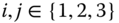
) for all three vehicles. The position of each UGV as they formed the desired triangle is shown in Figure 5.7, where the markers denote the vehicle location at different instants of time during the interval ![]() s. The inter‐vehicle distance errors defined in (2.6) are depicted in Figure 5.8, showing that the desired formation was acquired in less than 5 seconds. Notice from Figures 5.7 and 5.8 that the vehicles exhibit a small oscillatory motion near the final formation configuration. This is due to the fact that the formation acquisition objective is a setpoint control problem, therefore the vehicles are operating near zero velocity where static friction effects are prominent. Furthermore, the vehicles have noticeable backlash in the mechanical transmission. Since the encoder was collocated with the DC motor's drive shaft, these small position perturbations are measured by the encoder, but are often unobserved at the vehicle level due to the flexibility of the gear train.
s. The inter‐vehicle distance errors defined in (2.6) are depicted in Figure 5.8, showing that the desired formation was acquired in less than 5 seconds. Notice from Figures 5.7 and 5.8 that the vehicles exhibit a small oscillatory motion near the final formation configuration. This is due to the fact that the formation acquisition objective is a setpoint control problem, therefore the vehicles are operating near zero velocity where static friction effects are prominent. Furthermore, the vehicles have noticeable backlash in the mechanical transmission. Since the encoder was collocated with the DC motor's drive shaft, these small position perturbations are measured by the encoder, but are often unobserved at the vehicle level due to the flexibility of the gear train.

Figure 5.8Single integrator: formation acquisition. UGV distance errors  ,
,  .
.
The control voltages applied to the each vehicle's drive‐wheel DC motor is shown in Figure 5.9, and are well below the maximum battery voltage of 16 V. The constant switching observed in the voltages after the UGVs reach the desired formation is due to the static friction compensation term, ![]() , in (5.10a). Due to imperfect, noisy measurements,
, in (5.10a). Due to imperfect, noisy measurements, ![]() “chatters” about zero in the steady state and causes this term to constantly switch. The steering angle commands to the servo motors that orient the UGV front wheels are given in Figure 5.10, showing that they quickly became saturated at their maximum value of approximately
“chatters” about zero in the steady state and causes this term to constantly switch. The steering angle commands to the servo motors that orient the UGV front wheels are given in Figure 5.10, showing that they quickly became saturated at their maximum value of approximately ![]() . This saturation can be attributed to the vehicles being regulated to a setpoint position, which results in the vehicle longitudinal speed
. This saturation can be attributed to the vehicles being regulated to a setpoint position, which results in the vehicle longitudinal speed ![]() approaching zero. As
approaching zero. As ![]() decreases over time, the steering angle becomes larger according to (5.10b).
decreases over time, the steering angle becomes larger according to (5.10b).

Figure 5.9Single integrator: formation acquisition. Drive‐wheel DC motor voltages  ,
,  .
.

Figure 5.10Single integrator: formation acquisition. Steering angle commands  ,
,  .
.
Figure 5.11 displays the ![]() ‐ and
‐ and ![]() ‐direction components of the velocity error ( 5.13
) for each UGV. When tuning the control gain
‐direction components of the velocity error ( 5.13
) for each UGV. When tuning the control gain ![]() , a balance was struck between acceptable steady‐state performance and limiting the transient amplitude of the velocity errors.
, a balance was struck between acceptable steady‐state performance and limiting the transient amplitude of the velocity errors.

Figure 5.11Single integrator: formation acquisition. Velocity error  for each UGV along
  and
and  directions.
5.4.2 Single Integrator: Formation Maneuvering
Two formation maneuvering experiments were conducted: one with formation translation only, and the other with translation and rotation. In both experiments, the UGVs started in the initial configuration of ( 5.17
) while the control gains in (2.23) and ( 5.15
) were set to ![]() ,
, ![]()
![]()
![]() , and
, and ![]()
![]() .
.
Formation Translation: In this experiment, the UGVs were commanded to move north‐east along a bearing of approximately ![]() with a constant translational speed of 0.5 m/s while maintaining the inter‐vehicle distance of 4 m in the triangular formation. As a result, the desired translational and angular velocities in (2.24) became
with a constant translational speed of 0.5 m/s while maintaining the inter‐vehicle distance of 4 m in the triangular formation. As a result, the desired translational and angular velocities in (2.24) became ![]() m/s and
m/s and ![]() .
.
Figure 5.12 shows the position of each UGV as they maneuver on the plane, including snapshots of the actual formation at ![]() s and
s and ![]() s. Figure 5.13 shows the inter‐vehicle distance errors converging to a small steady‐state value after about 15 s.
s. Figure 5.13 shows the inter‐vehicle distance errors converging to a small steady‐state value after about 15 s.
![Graph with x - East (m) on the horizontal axis, y - North (m) on the vertical axis, initial and final formation marked in triangles for single integrator: formation translation. UGV position trajectories qi(t) = [xi(t), yi(t)], i = 1, 2, 3.](http://images-20200215.ebookreading.net/1/5/5/9781118887448/9781118887448__formation-control-of__9781118887448__images__c05f012.jpg)
Figure 5.12Single integrator: formation translation. UGV position trajectories  ,
,  .
.
Figure 5.13Single integrator: formation translation. UGV distance errors  ,
,  .
.
The actual translational speed and heading (bearing) angle of each UGV are displayed in Figure 5.14. At first glance, we can see that UGVs 1 and 3 converge to the desired translational speed of ![]() m/s and the desired bearing angle of
m/s and the desired bearing angle of ![]() , while UGV 2 appears to be moving in the wrong direction. However, based on Figures 5.12 and 5.13, we know that the desired formation maneuvering is achieved. Upon closer inspection, we observe that UGV 2's heading is approximately
, while UGV 2 appears to be moving in the wrong direction. However, based on Figures 5.12 and 5.13, we know that the desired formation maneuvering is achieved. Upon closer inspection, we observe that UGV 2's heading is approximately ![]() , which is
, which is ![]() from the desired heading. Therefore, the vehicle is moving in reverse in the direction that promotes the formation maneuvering control objective. This occurs because the formation maneuvering controller is only concerned with the relative position of the vehicles and does not actively control the heading of each vehicle. As a result, the controller may determine that it is beneficial (based on the commanded velocity and the vehicle's current position/heading) to operate in reverse mode.
from the desired heading. Therefore, the vehicle is moving in reverse in the direction that promotes the formation maneuvering control objective. This occurs because the formation maneuvering controller is only concerned with the relative position of the vehicles and does not actively control the heading of each vehicle. As a result, the controller may determine that it is beneficial (based on the commanded velocity and the vehicle's current position/heading) to operate in reverse mode.
Figure 5.14Single integrator: formation translation. UGV speeds and heading angles. The thick black lines denote the desired values.

Figure 5.15Single integrator: formation translation. Drive‐wheel DC motor voltages  ,
,  .
.

Figure 5.16Single integrator: formation translation. Steering angle commands  ,
,  .
.
The DC motor voltage of each vehicle is shown in Figure 5.15. One can observe a steady‐state voltage of ![]() V on each of the vehicles. This bias voltage is required to keep the vehicles moving at the desired translational speed of 0.5 m/s. Note that a negative voltage indicates that the vehicle is moving in reverse. Indeed, from Figure 5.12 we can see the moment where UGV 2 transitions from an initial forward motion to the reverse motion, which it maintains until the end of the experiment. On the other hand, UGV 3 does the opposite maneuver: initial reverse motion followed by forward motion. Clearly, the formation translational speed can be increased significantly since each UGV only utilized approximately 2 V
V on each of the vehicles. This bias voltage is required to keep the vehicles moving at the desired translational speed of 0.5 m/s. Note that a negative voltage indicates that the vehicle is moving in reverse. Indeed, from Figure 5.12 we can see the moment where UGV 2 transitions from an initial forward motion to the reverse motion, which it maintains until the end of the experiment. On the other hand, UGV 3 does the opposite maneuver: initial reverse motion followed by forward motion. Clearly, the formation translational speed can be increased significantly since each UGV only utilized approximately 2 V![]() V
V ![]() of the battery voltage. The somewhat slow translational speed was specifically chosen to maintain the vehicles operating at low velocities in case of hardware failure, and to prevent the vehicles from overrunning the parking lot area.
of the battery voltage. The somewhat slow translational speed was specifically chosen to maintain the vehicles operating at low velocities in case of hardware failure, and to prevent the vehicles from overrunning the parking lot area.
The steering angles are displayed in Figure 5.16. Notice that, aside from a brief period during the transient, the steering angles do not saturate as in Figure 5.10 because ![]() in (5.10b) never approaches zero during formation maneuvering. The steering angles of each UGV attain a steady‐state value of zero since the front‐wheel direction needs to eventually align with the
in (5.10b) never approaches zero during formation maneuvering. The steering angles of each UGV attain a steady‐state value of zero since the front‐wheel direction needs to eventually align with the ![]() ‐axis for the vehicle to move in the desired direction.
‐axis for the vehicle to move in the desired direction.
![Graph with x - East (m) on the horizontal axis, y - North (m) on the vertical axis, initial and final formation marked in triangles for single integrator: formation translation/rotation. UGV position trajectories qi(t) = [xi(t), yi(t)], i = 1, 2, 3.](http://images-20200215.ebookreading.net/1/5/5/9781118887448/9781118887448__formation-control-of__9781118887448__images__c05f017.jpg)
Figure 5.17Single integrator: formation translation/rotation. UGV position trajectories  ,
,  .
.

Figure 5.18Single integrator: formation translation/rotation. UGV distance errors  ,
,  .
.

Figure 5.19Single integrator: formation translation/rotation. UGV bearing rate  ,
,  .
.
Formation Translation and Rotation: Here, the formation had to move with the same translational velocity of the previous experiment while rotating about UGV 2 with an angular velocity of ![]() deg/s. Figure 5.17 depicts the propagation of the formation over time. Since UGV 2 is the axis of rotation, it merely translates in the north‐east direction while UGVs 1 and 3 trace a spiral‐like trajectory as they spin around UGV 2. The distance errors in Figure 5.18 indicate that the triangular formation was acquired by 10 s. In Figure 5.19, we can see the bearing rate
deg/s. Figure 5.17 depicts the propagation of the formation over time. Since UGV 2 is the axis of rotation, it merely translates in the north‐east direction while UGVs 1 and 3 trace a spiral‐like trajectory as they spin around UGV 2. The distance errors in Figure 5.18 indicate that the triangular formation was acquired by 10 s. In Figure 5.19, we can see the bearing rate ![]() of UGVs 1 and 3 converging to the desired angular velocity of 20 deg/s. This angle rate was calculated by numerically differentiating the vehicle's measured bearing
of UGVs 1 and 3 converging to the desired angular velocity of 20 deg/s. This angle rate was calculated by numerically differentiating the vehicle's measured bearing ![]() with all discontinuities removed (i.e., when the vehicles' magnetic heading value transitioned from
with all discontinuities removed (i.e., when the vehicles' magnetic heading value transitioned from ![]() to
to ![]() ).
).
The velocity error of each UGV is shown in Figure 5.20. The smaller error for UGV 2 is expected since its desired velocity is constant (setpoint problem) whereas the desired velocities for UGVs 1 and 3 are time varying (tracking problem). The drive‐wheel motor voltages and steering angles are given in Figures 5.21 and 5.22, respectively. From Figure 5.21, we can see that UGV 2 was operating in reverse throughout the experimental trial since its voltage was always negative. Notice the nonzero steady‐state values of the steering angles for UGVs 1 and 3 required for producing the rotation about UGV 2. On the other hand, the steering angle of UGV 2 reaches zero at ![]() s when the vehicle becomes aligned with the direction of translational velocity vector
s when the vehicle becomes aligned with the direction of translational velocity vector ![]() .
.

Figure 5.20Single integrator: formation translation/rotation. Velocity error  of each UGV along the
  and
and  directions.

Figure 5.21Single integrator: formation translation/rotation. Drive‐wheel DC motor voltages  ,
,  .
.

Figure 5.22Single integrator: formation translation/rotation. Steering angle commands  ,
,  .
.
5.4.3 Single Integrator: Target Interception
For this experiment a virtual vehicle was employed as the target since additional UGVs were not available. The target's translational speed was set to a constant value of ![]() m/s and its heading angle to an oscillatory motion of
m/s and its heading angle to an oscillatory motion of ![]() deg. The same triangular formation from Section 5.4.2 was used. The target velocity estimate
deg. The same triangular formation from Section 5.4.2 was used. The target velocity estimate ![]() in (2.45) was initialized to zero and was calculated using the trapezoidal rule of integration. The control gains were set to
in (2.45) was initialized to zero and was calculated using the trapezoidal rule of integration. The control gains were set to ![]() and
and ![]() in (2.53) and (2.54), and
in (2.53) and (2.54), and ![]() and
and ![]() in ( 5.15
). Since only three vehicles were available, UGV 2 was selected as the leader of the formation, i.e., the agent responsible for chasing the target. As a result, the target interception error (2.44) was defined as
in ( 5.15
). Since only three vehicles were available, UGV 2 was selected as the leader of the formation, i.e., the agent responsible for chasing the target. As a result, the target interception error (2.44) was defined as ![]() , and the target was located at the boundary of the formation when intercepted.
, and the target was located at the boundary of the formation when intercepted.
Figure 5.23 shows the motions of the UGVs and target over time. The inter‐vehicle distance errors and the target interception error defined in (2.44) are given in Figures 5.24 and 5.25, respectively. From these figures, one can see that the target was successfully intercepted after approximately 10 s while the formation was acquired after 20 s.

Figure 5.23Single integrator: target interception. UGV position trajectories  ,
,  and target position
  . Target was initially positioned at
  m.
m.

Figure 5.24Single integrator: target interception. UGV distance errors  ,
,  .
.
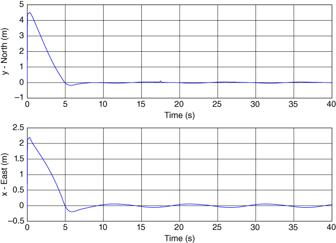
Figure 5.25Single integrator: target interception. Target interception error  .
.
Figure 5.26 displays the drive‐wheel motor voltage for each vehicle. As in the formation maneuvering experiment, the voltages reach a steady‐state value of ![]() V since the formation needs to track the target's translational velocity of
V since the formation needs to track the target's translational velocity of ![]() m/s. The steering angles, shown in Figure 5.27, have an oscillatory motion for
m/s. The steering angles, shown in Figure 5.27, have an oscillatory motion for ![]() s because of the sinusoidal heading movement of the target. That is, the oscillation period is 10 s, which corresponds to the frequency of the target's heading motion (0.1 Hz).
s because of the sinusoidal heading movement of the target. That is, the oscillation period is 10 s, which corresponds to the frequency of the target's heading motion (0.1 Hz).

Figure 5.26Single integrator: target interception. Drive‐wheel DC motor voltages  ,
,  .
.

Figure 5.27Single integrator: target interception. Steering angle commands  ,
,  .
.
5.4.4 Single Integrator: Dynamic Formation
For the following experiment, the desired formation was set to a time‐varying version of the one used in the previous experiments. Specifically, we used an equilateral triangle with time‐varying inter‐vehicle distances specified as
In addition, we required the formation to maneuver according to the translation described in the first experiment of Section 5.4.2. The vehicles were again initially located according to ( 5.17
), and the control gains were tuned to ![]() in (2.73), and
in (2.73), and ![]() and
and ![]() in ( 5.15
).
in ( 5.15
).

Figure 5.28Single integrator: dynamic formation. UGV position trajectories  ,
,  .
.
The trajectory of each UGV along with snapshots of the formation at instants of minimum and maximum values for (5.19) are given in Figure 5.28. It is interesting to note that UGV 1 strictly followed the desired translation with virtually no oscillations, while UGVs 2 and 3 appear to carry the brunt of the effort to track the sinusoidal dynamic formation. From the distance errors in Figure 5.29, we see that the desired formation was acquired and tracked after about 15 s with a steady‐state error within ![]() cm.
cm.

Figure 5.29Single integrator: dynamic formation. UGV distance errors  ,
,  .
.
The drive‐wheel motor voltages in Figure 5.30 again converge to ![]() V as needed to move the vehicles with
V as needed to move the vehicles with ![]() m/s speed. In this experiment, the voltages were saturated to
m/s speed. In this experiment, the voltages were saturated to ![]() of the maximum battery voltage (8 V). Note that UGV 2 moved in reverse for the entire duration of the experimental run. The steering angles are displayed in Figure 5.31. It was mentioned previously that UGV 1 moved in a fairly straight positional track as compared to UGVs 2 and 3. This observation is substantiated by noting that UGV 1's steering angle has much smaller oscillations about
of the maximum battery voltage (8 V). Note that UGV 2 moved in reverse for the entire duration of the experimental run. The steering angles are displayed in Figure 5.31. It was mentioned previously that UGV 1 moved in a fairly straight positional track as compared to UGVs 2 and 3. This observation is substantiated by noting that UGV 1's steering angle has much smaller oscillations about ![]() as compared to UGVs 2 and 3.
as compared to UGVs 2 and 3.

Figure 5.30Single integrator: dynamic formation. Drive‐wheel DC motor voltages  ,
,  .
.

Figure 5.31Single integrator: dynamic formation. Steering angle commands  ,
,  .
.
5.4.5 Double Integrator: Formation Acquisition
In order to enable the proper comparison between the double integrator (DI)‐based formation acquisition controller and the single integrator (SI)‐based one, the control gain ![]() in (3.9) was set to the same value reported in Section 5.4.1, while we used
in (3.9) was set to the same value reported in Section 5.4.1, while we used ![]() in (3.8), which is the same value as
in (3.8), which is the same value as ![]() of ( 5.15
) in the experiment of Section 5.4.1.
of ( 5.15
) in the experiment of Section 5.4.1.
The UGV trajectories from their initial configuration to the final configuration are displayed in Figure 5.32, while the inter‐vehicle distance errors are shown in Figure 5.34. In Figure 5.33, we replot the trajectories of both the DI‐ and SI‐based controllers to facilitate the comparison. First, one can see that the final formations are isomorphic according to Definition 1.4. Note that the DI‐based controller produced a more irregular response than the SI one. This is more clearly seen by the side‐by‐side comparison of the distance errors in Figure 5.35, where the response of the DI‐based controller is noticeably less damped. We believe that this is due to the control gains in (3.8) and (3.9) not being retuned for the DI system, whose closed‐loop dynamics have higher order than the SI dynamics. From the inset plots in Figures 5.8 and 5.34, we can see that the steady‐state errors of the DI‐based control were slightly smaller in their peak‐to‐peak amplitude than those of the SI‐based control. Again, better tuning of DI‐based control gains could result in even better steady‐state performance.

Figure 5.32Double integrator: formation acquisition. UGV position trajectories  ,
,  .
.

Figure 5.33Comparison of UGV position trajectories.

Figure 5.34Double integrator: formation acquisition. UGV distance errors  ,
,  .
.

Figure 5.35Comparison of distance errors.
The motor voltages, which are shown in Figure 5.36, have larger transient magnitudes than those of the SI‐based controller (see Figure 5.9); however, the steady‐state magnitudes are only slightly larger. This suggests that the DI‐based formation acquisition controller required more control energy than its SI counterpart. The steering angles in Figure 5.37 are qualitatively similar to the ones for the SI‐based control (see Figure 5.10) in the sense that they operated in saturation for the duration of the experiment due to the UGV longitudinal speed ![]() quickly converging to zero.
quickly converging to zero.

Figure 5.36Double integrator: formation acquisition. Drive‐wheel DC motor voltages  ,
,  .
.

Figure 5.37Double integrator: formation acquisition. Steering angle commands  ,
,  .
.
5.4.6 Double Integrator: Formation Maneuvering
The same translation‐only maneuvering experiment described in Section 5.4.2 was run with the DI‐based controller. The same control gain values given in Section 5.4.5 were used in (3.17). In order to provide compensation for the uphill grade of the parking lot, the original DI‐based control (3.8) was augmented with the following integral feedback term:

where ![]() was set to 0.5 for this experiment. This term is akin to the one used in ( 5.15
) for implementation of the SI‐based controllers.
was set to 0.5 for this experiment. This term is akin to the one used in ( 5.15
) for implementation of the SI‐based controllers.
Figure 5.38 displays the movement of the formation during the 40‐s experimental run, and Figure 5.39 compares it to the SI‐based control. The trajectories of UGVs 1 and 3 were very similar between the two schemes, while UGV 2 moved initially in opposite directions but then converged to a common trajectory. The distance errors are shown in Figure 5.40, and their comparison with the SI errors are given in Figure 5.41. We again observe the less damped response of the DI errors, which are attributed to the control gains not being fine tuned for the DI dynamics. Indeed, when we calculated the RMS value of the inter‐vehicle distance error vector, ![]() , defined by
, defined by

where ![]() s is the final experiment time, we obtained
s is the final experiment time, we obtained ![]() for the DI controller as compared to 0.641 when the SI controller was employed.
for the DI controller as compared to 0.641 when the SI controller was employed.

Figure 5.38Double integrator: formation maneuvering. UGV position trajectories  ,
,  .
.

Figure 5.39Comparison of UGV position trajectories.
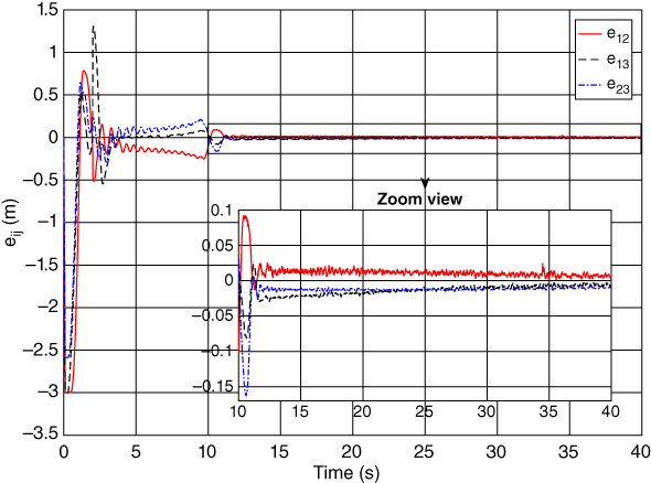
Figure 5.40Double integrator: formation maneuvering. UGV distance errors  ,
,  .
.

Figure 5.41Comparison of distance errors.

Figure 5.42Double integrator: formation maneuvering. Velocity error  of each UGV along the
  and
and  directions.
The velocity error variable ![]() defined in (3.4) is shown in Figure 5.42 for each UGV and converges to zero as predicted by the theory. The motor voltages, displayed in Figure 5.43, have more oscillations and larger magnitude during the transient period than the SI voltages (see Figure 5.15), but naturally have the same steady‐state value of
defined in (3.4) is shown in Figure 5.42 for each UGV and converges to zero as predicted by the theory. The motor voltages, displayed in Figure 5.43, have more oscillations and larger magnitude during the transient period than the SI voltages (see Figure 5.15), but naturally have the same steady‐state value of ![]() V corresponding to the 0.5 m/s translational speed of the maneuver. Note that the oscillations occurred about zero, indicating that the vehicles switched between forward and reverse motions during the first 8–10 s and then settled to one or the other (UGV 1 reverse; UGV 2 reverse; UGV 3 forward) until the end of the experiment. The steering angles in Figure 5.44 are much noisier than the SI ones in Figure 5.16. We believe the DI voltages and steering angles would look similar to their SI counterparts if the control gains were retuned for the DI dynamics.
V corresponding to the 0.5 m/s translational speed of the maneuver. Note that the oscillations occurred about zero, indicating that the vehicles switched between forward and reverse motions during the first 8–10 s and then settled to one or the other (UGV 1 reverse; UGV 2 reverse; UGV 3 forward) until the end of the experiment. The steering angles in Figure 5.44 are much noisier than the SI ones in Figure 5.16. We believe the DI voltages and steering angles would look similar to their SI counterparts if the control gains were retuned for the DI dynamics.

Figure 5.43Double integrator: formation maneuvering. Drive‐wheel DC motor voltages  ,
,  .
.

Figure 5.44Double integrator: formation maneuvering. Steering angle commands  ,
,  .
.
5.4.7 Double Integrator: Target Interception
The following experiment utilized the same trial conditions as the experiment in Section 5.4.3 with the exception that the target velocity ![]() was assumed to be known by the vehicles as per the assumption in Section 3.4. The control law given by (3.19), (3.20), (3.21), and ( 5.12
) was implemented with the addition of the integral feedback term
was assumed to be known by the vehicles as per the assumption in Section 3.4. The control law given by (3.19), (3.20), (3.21), and ( 5.12
) was implemented with the addition of the integral feedback term ![]() (as was done in (5.20)) and with control gains set to
(as was done in (5.20)) and with control gains set to ![]() ,
, ![]() ,
, ![]() ,
, ![]() , and
, and ![]() . Notice that the control gain
. Notice that the control gain ![]() that multiplies the discontinuous term sgn
that multiplies the discontinuous term sgn![]() in (3.19) was set to zero in the experiment. During tuning trials, it was observed that larger values of
in (3.19) was set to zero in the experiment. During tuning trials, it was observed that larger values of ![]() caused the UGVs to jitter; thus, the variable structure‐type term was turned off. However, this term would be beneficial if the target motion was more aggressive since it would enable faster reactions from the chasing vehicles.
caused the UGVs to jitter; thus, the variable structure‐type term was turned off. However, this term would be beneficial if the target motion was more aggressive since it would enable faster reactions from the chasing vehicles.
Figure 5.45 shows the trajectories of the UGVs and virtual target. Figures 5.46 and 5.47 display the inter‐vehicle distance errors and target interception error, respectively. These results show that while the desired formation was acquired relatively quickly (by 10 s), the target was only intercepted by UGV 2 after 25 s. The settling time of the target interception error may be explained by the behavior of the velocity error ![]() in Figure 5.48, which also has a settling time of 25 s. This settling time could be shorten by increasing the integral feedback gain
in Figure 5.48, which also has a settling time of 25 s. This settling time could be shorten by increasing the integral feedback gain ![]() from its original value of 0.5 (recall that consistency of control gain values between the various experiments was used to facilitate their comparison). In contrast to the SI target interception error, which exhibited some small steady‐state oscillations about zero (see Figure 5.25), the DI target interception error converged to zero with virtually no steady‐state offset. This is likely due to the target velocity being known to the DI‐based control whereas it was estimated in the SI‐based control. As for the inter‐vehicle distance errors, the SI and DI controllers yielded similar steady‐state values within
from its original value of 0.5 (recall that consistency of control gain values between the various experiments was used to facilitate their comparison). In contrast to the SI target interception error, which exhibited some small steady‐state oscillations about zero (see Figure 5.25), the DI target interception error converged to zero with virtually no steady‐state offset. This is likely due to the target velocity being known to the DI‐based control whereas it was estimated in the SI‐based control. As for the inter‐vehicle distance errors, the SI and DI controllers yielded similar steady‐state values within ![]() cm.
cm.

Figure 5.45Double integrator: target interception. UGV position trajectories  ,
,  and target position
  . The target was initially positioned at
  m.
m.

Figure 5.46Double integrator: target interception. UGV distance errors  ,
,  .
.

Figure 5.47Double integrator: target interception. Target interception error  .
.

Figure 5.48Double integrator: target interception. Velocity error  of each UGV along the
  and
and  directions.

Figure 5.49Double integrator: target interception. Drive‐wheel DC motor voltages  ,
,  .
.

Figure 5.50Double integrator: target interception. Steering angle commands  ,
,  .
.
The voltages and steering angles are given in Figures 5.49 and 5.50, respectively. In this experiment, the voltages were restricted to ![]() of the maximum battery voltage (approximately
of the maximum battery voltage (approximately ![]() V) to limit the vehicles' velocity to within manageable limits (
V) to limit the vehicles' velocity to within manageable limits (![]() m/s) so that the vehicles stayed within the testing area. As such, the voltages saturated during the first 3 s of the experiment since the transient period is usually the most demanding from the control energy perspective. The DI steering angles are noticeably noisier than the SI ones in Figure 5.27, although one can still distinguish the 10 Hz oscillation caused by the sinusoidal variation of the target heading angle.
m/s) so that the vehicles stayed within the testing area. As such, the voltages saturated during the first 3 s of the experiment since the transient period is usually the most demanding from the control energy perspective. The DI steering angles are noticeably noisier than the SI ones in Figure 5.27, although one can still distinguish the 10 Hz oscillation caused by the sinusoidal variation of the target heading angle.

Figure 5.51Double integrator: dynamic formation. UGV position trajectories  ,
,  .
.
5.4.8 Double Integrator: Dynamic Formation
This experiment was conducted using the same formation objectives as Section 5.4.4. The integral feedback term was also included (3.8), as in the previous two DI experiments with control gains set to ![]() ,
, ![]() , and
, and ![]() .
.
The results of the DI‐based dynamic formation controller are shown in Figures 5.51 to 5.56 along with comparisons with the SI‐based control. Unlike in the SI experiment, UGV 1 did not strictly follow the desired translation and exhibited small oscillations in its heading angle. This is also evidenced by the oscillations of its steering angle seen in Figure 5.56 in comparison to the other UGVs. The settling time and overshoot of the distance errors were smaller for the DI control, although the response was less damped. The DI control also produced smaller steady‐state errors, as can be seen by comparing the insets of Figures 5.53 and 5.29. A comparison of the RMS value of the errors given by (5.21) resulted in ![]() for the DI controller and 0.929 for the SI controller. From the drive‐wheel motor voltages in Figure 5.55, we can see that the vehicles had more irregular (forward‐reverse) motions than when the SI‐based control was used (see Figure 5.30 for comparison). Finally, the UGV steering angles of the DI‐based control had larger high‐frequency variations than those of the SI case.
for the DI controller and 0.929 for the SI controller. From the drive‐wheel motor voltages in Figure 5.55, we can see that the vehicles had more irregular (forward‐reverse) motions than when the SI‐based control was used (see Figure 5.30 for comparison). Finally, the UGV steering angles of the DI‐based control had larger high‐frequency variations than those of the SI case.

Figure 5.52Figure 5.52Comparison of UGV position trajectories.

Figure 5.53Double integrator: dynamic formation. UGV distance errors  ,
,  .
.

Figure 5.54Figure 5.54Comparison of distance errors.

Figure 5.55Double integrator: dynamic formation. Drive‐wheel DC motor voltages  ,
,  .
.

Figure 5.56Double integrator: dynamic formation. Steering angle commands  ,
,  .
.
5.4.9 Holonomic Dynamics: Formation Acquisition
Finally, we tested the adaptive controller presented in Section 4.3.2, which is based on the holonomic dynamics of the UGVs. The hand position of each UGV was set to ![]() m,
m, ![]() , which is the same value as
, which is the same value as ![]() in (5.9). The torque‐level control law in (4.30a) was augmented with the integral feedback term
in (5.9). The torque‐level control law in (4.30a) was augmented with the integral feedback term ![]() . The control and adaptation gains in (4.30) and (2.15) were chosen as
. The control and adaptation gains in (4.30) and (2.15) were chosen as ![]() ,
, ![]() ,
, ![]() , and
, and ![]() . In addition, the 18 components of the parameter estimate vector
. In addition, the 18 components of the parameter estimate vector ![]() were initialized to zero.
were initialized to zero.
The motion of the UGVs from the initial formation until the desired formation was acquired is shown in Figure 5.57. From Figure 5.58, we can see that the desired formation was reached within 5 s. The comparison with the SI‐ and DI‐based formation acquisition controllers in Figure 5.59 shows that the response of the adaptive controller was the most damped. In fact, the RMS value of the inter‐vehicle distance error given in ( 5.21 ) for the three controllers resulted in 0.835 (holonomic), 0.688 (SI), and 0.629 (DI). The higher value of the holonomic‐based controller is obviously due to its slower response. However, it is possible that the response can be sped up in a critically damped fashion by additional tuning of the control gains. That is, gain tuning is facilitated in this case by the fact that the adaptive controller—given its certainty equivalence‐like structure—is quasi‐feedback linearizing the hand dynamics (4.19).
![Graph with x - East (m) on the horizontal axis, y - North (m) on the vertical axis, initial and final formation marked in triangles for qi(t) = [xi(t), yi(t)], i = 1, 2, 3 and points plotted for UGV 1, UGV 2, and UGV 3.](http://images-20200215.ebookreading.net/1/5/5/9781118887448/9781118887448__formation-control-of__9781118887448__images__c05f057.jpg)
Figure 5.57Holonomic dynamics: formation acquisition. UGV position trajectories  ,
,  .
.
Figure 5.58Holonomic dynamics: formation acquisition. UGV distance errors  ,
,  .
.

Figure 5.59Comparison of distance errors.
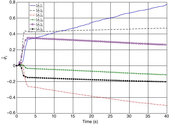
Figure 5.60Holonomic dynamics: formation acquisition. Parameter estimates for UGV 1,  .
.
For illustration purposes, the six parameter estimates of UGV 1 only are displayed in Figure 5.60. One can observe that the parameter estimates—most notably ![]() and
and ![]() —are drifting. The drift is caused by the adaptation law of (4.30b) being primarily driven by the velocity error signal
—are drifting. The drift is caused by the adaptation law of (4.30b) being primarily driven by the velocity error signal ![]() which does not converge exactly to zero, as shown in Figure 5.61. Since in the pure formation acquisition problem the vehicles operate near zero velocity at steady state, they are subject to noticeable static friction affects. Although the low‐level controller attempts to compensate for static friction, the vehicles still tend to jitter about the desired setpoint, as can be seen from the steady‐state oscillations in the inset of Figure 5.58. As a result, these oscillations cause the parameter estimates to continue to update. If the experiment were conducted with formation maneuvering, one may not observe the parameter estimate drift. Furthermore, one can always modify the adaptation law with one of the numerous methods for bounding the parameter estimates (e.g., dead zone,
which does not converge exactly to zero, as shown in Figure 5.61. Since in the pure formation acquisition problem the vehicles operate near zero velocity at steady state, they are subject to noticeable static friction affects. Although the low‐level controller attempts to compensate for static friction, the vehicles still tend to jitter about the desired setpoint, as can be seen from the steady‐state oscillations in the inset of Figure 5.58. As a result, these oscillations cause the parameter estimates to continue to update. If the experiment were conducted with formation maneuvering, one may not observe the parameter estimate drift. Furthermore, one can always modify the adaptation law with one of the numerous methods for bounding the parameter estimates (e.g., dead zone, ![]() ‐modification,
‐modification, ![]() ‐modification, and projection operators 123, 124).
‐modification, and projection operators 123, 124).

Figure 5.61Holonomic dynamics: formation acquisition. Velocity error  of each UGV along the
  and
and  directions.
The drive‐wheel voltages and steering angles commands are given in Figures 5.62 and 5.63, respectively. As expected, the voltages are constantly switching after the formation is acquired, albeit at a higher frequency than in the SI and DI formation acquisition experiments. This higher frequency can also be observed in the steering angles. This behavior means that the UGVs experienced a stronger jitter about the desired formation with the adaptive controller.

Figure 5.62Holonomic dynamics: formation acquisition. Drive‐wheel DC motor voltages  ,
,  .
.

Figure 5.63Holonomic dynamics: formation acquisition. Steering angle commands  ,
,  .
.
5.4.10 Summary
The above experimental results provide a baseline for understanding the performance of graph rigidity‐based formation controllers. Naturally, the results can be improved by employing better hardware (e.g., more powerful processor, higher resolution optical encoder, wireless router with higher baud rate), more exhaustive control gain tuning, and a more accurate vehicle model. Nevertheless, a few conclusions can be drawn from the experimental results.
First, the desired formation is easier to obtain when the vehicles are moving (formation maneuvering problem) because static friction is a prominent factor in the stationary case (pure formation acquisition problem). Therefore, adequate static friction compensation is imperative for high‐precision applications of UGV formations. Despite the control gains in this experimental study being tuned for the SI‐based controllers, the other controllers produced comparable performance. Therefore, there is greater room for improvement in the performance of the DI‐ and holonomic dynamics‐based controllers by better gain tuning. It should be noted that although the control gains have a PID‐like interpretation their tuning is not straightforward since the closed‐loop system is nonlinear.
Setpoint control problems, such as the formation acquisition problem, can lead to poor transient behavior due to the initial jump of step‐like command. One way of improving the transient performance of the formation acquisition controllers is to set the desired distance to the time‐varying function, ![]() where
where ![]() is a design parameter and
is a design parameter and ![]() is the final desired distance. This function creates a smooth step function with zero initial error.
is the final desired distance. This function creates a smooth step function with zero initial error.
Finally, independent of what control technique is employed, the importance of a reliable communication system for high‐performance formation control cannot be overstated.