C.1 Linear Systems

The following material can be found in 129, 130. Given a real function of time satisfying the condition

for some finite real , its Laplace transform is defined as

where (complex number) is called the Laplace variable.

Two important properties of the Laplace transform are

Roughly speaking, the above properties indicate that multiplication by in the Laplace domain is equivalent to the differential operator in the time domain (). Likewise, division by in the Laplace domain is equivalent to the integral operator in the time domain ().

Consider the single‐input/single‐output (SISO), linear time‐invariant (LTI) system

with initial conditions , where and are real constants, is the scalar output, and is the scalar input. The transfer function of the system is defined as the ratio of the Laplace transform of the output over the Laplace transform of the input, with all initial conditions assumed to be zero. That is,

In general, if an LTI system has inputs and outputs, the transfer function between the th input and the th output is defined as

with , , (i.e., all inputs other than the th are set to zero). In matrix‐vector form, we then have that

where , , and

is the transfer function matrix.

The following theorem is a valuable result for input‐output stability.

• If , then , , is continuous, and as .
• If , then , , and is uniformly continuous. If, in addition, as , then as .

C.2 Nonlinear Systems

The following material can be found in 8,9,131. Consider the nonautonomous (time‐varying) system

(C.1)

where is locally Lipschitz in and piecewise continuous in on . Since is in general a nonlinear function of and , we seek to qualify the stability properties of C.1.

The first step in this analysis is to determine the equilibrium points of the system. A point is an equilibrium point of C.1 at if it has the property that whenever the system state starts at the equilibrium, it remains at the equilibrium for all . Mathematically, this means that equilibrium points can be found by solving the algebraic equation

A nonlinear system may have a unique equilibrium point, a finite number of equilibrium points, or an infinite number of equilibrium points. In the case of multiple equilibrium points, each one could have a different stability property. The issue of stability deals with the behavior of the solutions of C.1 for initial conditions away from an equilibrium point (i.e., ). That is, does an equilibrium point attract the solution, repel the solution, or neither (e.g., a periodic solution). It is standard practice in stability analysis to shift a nonzero equilibrium point of interest to the origin through the variable transformation

such that C.1 with equilibrium point is equivalent to with equilibrium point . Henceforth, we will assume 0 is an equilibrium point of C.1.

Let the set

(C.2a)C.2a

represent the “ball” of radius centered at . Stability properties of the equilibrium point of C.1 are said to hold:

• locally if they are true for all
• globally if they are true for all ¹
• semi‐globally if they are true for all with arbitrary
• uniformly if they are true for all initial times .

The stability properties of the controllers developed in this book are true only locally.

The equilibrium point of C.1 is said to be:

• uniformly stable if, given any , there exists (independent of ) such that
  
• unstable if it is not stable
• uniformly convergent if there exists such that
  
• uniformly asymptotically stable if it is both uniformly stable and uniformly convergent
• exponentially stable if there exist such that
  (C.3)

Autonomous (time‐invariant) systems are a special case of C.1 where the right‐hand side of the differential equation is not explicitly dependent on time, i.e., . Therefore, equilibrium points of autonomous systems are always constant (time independent). Since the solution of an autonomous system depends only on , the stability properties of its equilibrium points are always uniform and can be taken as zero without loss of generality. For similar reasons, the qualifier “uniform” is not necessary when referring to the exponential stability of nonautonomous systems (notice that appears in C.3).

C.3 Lyapunov Stability

The following material can be found in 8,9,131,132. Lyapunov theory enables one to qualitatively assess the stability properties of an equilibrium point of interest without having to explicitly solve the nonlinear differential equation C.1. Specifically, the so‐called Lyapunov's second (or direct) method is based on the following, fundamental physical observation 132: If a system's total energy is continuously dissipated, then the system must eventually settle down to an equilibrium point. That is, equilibrium points are zero‐energy points. Since energy is a scalar quantity, we can study the stability of a system by examining the time variation of a single scalar function that captures the total energy of the system. In the case of mechanical systems (which multi‐agent systems fall under), this function should be related to the potential energy (position dependent) and kinetic energy (velocity dependent). This energy‐like function is known as the Lyapunov function candidate.

The notion of positive definite functions (and its variants) plays an important role in Lyapunov's second method. A function where is said to be:

• positive definite in if for all and
• positive semi‐definite in if for all and
• negative definite in if is positive definite
• negative semi‐definite in if is positive semi‐definite.

The simplest and most important type of positive definite function is the so‐called quadratic function:

where is symmetric. In the case of quadratic functions, checking the sign definiteness of is quite easy. Specifically, (or matrix ) is:

• positive definite if all eigenvalues of are positive
• positive semi‐definite if all eigenvalues of are nonnegative
• negative definite if all eigenvalues of are negative
• negative semi‐definite if all eigenvalues of are nonpositive
• indefinite if some eigenvalues of are positive and some are negative.

We are now ready to state some Lyapunov stability results. These results are based on the simple mathematical fact that if a scalar function is both bounded from below and decreasing, the function has a limit as time approaches infinity. In the following, we assume is an equilibrium point for C.1 and is a set containing .

The following theorem is a corollary to Barbalat's Lemma.

C.4 Input‐to‐State Stability

The following material can be found in 133,134. Input‐to‐state stability bridges the gap between the notions of Lyapunov stability and input–output stability by quantifying the effects of both initial conditions and external (control or disturbance) inputs on the system state.

Consider the system

(C.4)

where is locally Lipschitz in and . The input is a piecewise continuous, bounded function for all . System C.4 is said to be input‐to‐state stable if there exist a class function and a class function such that, for any and any , the solution exists for all and satisfies

(C.5)

The above inequality has several implications.

• For any bounded input, the state is bounded.
• As , the state is ultimately bounded by function .
• If as , so does .

C.5 Nonsmooth Systems

The following material can be found in 38, 42, 135, 136. Consider system

(C.7)

where is discontinuous in and piecewise continuous in on . Unfortunately, classical analysis methods are not applicable to differential equations with discontinuous right‐hand side (a.k.a. nonsmooth systems) since they require to be at least Lipschitz in . For such differential equations, even the notion of existence of solutions has to be redefined. A key contribution to this problem was made by Filippov, who developed a solution concept that only requires to be Lebesgue measurable with respect to and . This solution is usually called a generalized or Filippov solution. The discontinuities that appear in in this book are of the type which admit a Filippov solution.

A Filippov solution is found by embedding into a set‐valued map , and then investigating the existence of a solution to the so‐called differential inclusion

A natural choice for this set‐valued map is the closed convex hull of . If for any , , then is an equilibrium point of C.7.

In order to conduct a Lyapunov analysis of equilibria of a differential inclusion, we can invoke the following result from 42.

C.6 Integrator Backstepping

The following material can be found in 8,9,131. Integrator backstepping is a recursive control design methodology for systems in so‐called strict‐feedback form 9. It provides a systematic way of designing Lyapunov functions and nonlinear controllers for systems of any order. Unlike the feedback linearization method, backstepping can accommodate model uncertainties and avoid the unnecessary cancellation of “useful” (stabilizing) nonlinearities.

Since the dynamic model of the individual agents in this book have at most order two, we illustrate the backstepping technique by considering the system

(C.8)

(C.9)

where is the system state, is the control input, and is continuously differentiable with . Say that our control objective is to stabilize the system at the equilibrium point for any initial conditions.

Notice that the above system is a cascaded connection of subsystems C.8 and C.9. The idea behind backstepping is to first consider as a control input for subsystem C.8. Under this assumption, we could design to obtain the exponentially stable closed‐loop system . Since in reality is a system state and thus cannot be directly manipulated, we use the trick of adding and subtracting a fictitious control input to the right‐hand side of C.8 and introducing the variable transformation

As a result, our system becomes

Now, if we design

(C.10)

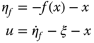
where

we get the closed‐loop system

(C.11)

whose unique equilibrium point is .

Using the Lyapunov function candidate

and taking its time derivative along C.11 yields

From Corollary C.1, we can conclude that is exponentially stable. Since , we know that is an exponentially stable equilibrium point for C.8 and C.9 in closed‐loop with C.10.