
Chapter 18
Matrix Math
What we'll cover in this chapter:
- Matrix basics
- Matrix operations
- Canvas transforms
Although this chapter does not introduce any new types of motion or methods of rendering graphics, it does introduce matrices, which provide an alternative way of applying visual transformations, something we've done throughout the book.
Matrices are used quite often in 3D systems for rotating, scaling, and translating (moving) 3D points. They are also used quite a bit in various 2D graphics transformations. In this chapter, you see how to create a system of matrices to manipulate objects and look at several methods built into the canvas that are used to work with matrices.
Matrix basics
A matrix, by simplest definition, is a grid of numbers. It can have one or more horizontal rows and one or more vertical columns. Figure 18-1 shows some matrices.
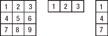
Figure 18-1. A 3 × 3 matrix, a 1 × 3 matrix, and a 3 × 1 matrix; each uses the rows by columns notation.
Any particular matrix is usually represented by a variable, such as M. To refer to a specific cell in a matrix, you use the variable name with the row and column number in subscript. For example, if the 3 × 3 matrix in Figure 18-1 is denoted as M, then using the rows by colums notation, M2,3 is equal to 6, as it refers to the second row, third column. Matrix indices start at 1, which is different than the notation for JavaScript arrays, which start at 0.
The cells of a matrix can contain not only numbers, but also formulas and variables. If you've ever used a spreadsheet, it is basically one big matrix. You can have one cell hold the sum of a column, and another cell multiply that sum by some number that's held in another cell, and so on. So, you see that matrices can be rather useful.
Matrix operations
A spreadsheet is kind of a free-form matrix, but the matrices we use are a lot more structured and have all kinds of rules for what we can do with them and how to do those things.
There are usually two ways to teach matrix math. The first approach describes how to do the operations in detail, using matrices full of seemingly random numbers. You learn the rules, but you have no idea why you are doing certain things or what the result means. It's like playing a game where you arrange the numbers in a pretty pattern.
The second approach is to describe the contents of the matrices in detail and skim over the operation. Using vague instructions such as “and then you just multiply these two matrices together and get this …”, leaving the reader with no idea how this multiplication is done.
In this chapter, we walk the line between these two methods. We start by looking at matrices that contain meaningful values, and then we see how to manipulate them.
Matrix addition
One of the more common uses of matrices is manipulating 3D points, which contain a value for its x, y, and z positions. We can easily view this as a 1 × 3 matrix, like so:
x y z
To move this point in space—also called translating the point—you need to know how far to move it on each axis. You can put this in a translation matrix, which is another 1 × 3 matrix that looks something like this:
Here, dx, dy, and dz are the distances to move on each axis. Now you need to apply the transformation matrix to the point matrix; this is done with matrix addition. You just add each corresponding cell together to make a new matrix containing the sum of each cell. To add two matrices, they need to be the same size. So for translation, you do this:
x y z + dx dy dz = (x + dx) (y + dy) (z + dz)
The resulting matrix can be called x1, y1, z1, and it contains the new position of the point after it has been translated. So, if you had a point at 100, 50, 75 on x, y, z, and then wanted to move it -10, 20, -35, here's how that would look:
100 50 75 + -10 20 -35 = (100 - 10) (50 + 20) (75 - 35)
Thus, when you perform the addition, you get 90, 70, 40 as the point's new position. You probably already noticed the correlation to velocity, where the velocity on each axis is added to the position on that axis. It's the same here, but we're just looking at it a bit differently.
If you had a larger matrix, you would still use the same process, matching up the cells. We won't be dealing with matrix addition for anything larger than 1 × 3 matrices here, but here's an abstract example:
a b c     j k l     (a + j) (b + k) (c + l)

d e f  +  m n o  =  (d + m) (e + n) (f + o)

g h i     p q r     (g + p) (h + q) (i + r)
That's all you need to know about matrix addition. After we cover matrix multiplication, you see how to put together some actual functions to use in a matrix-based 3D engine.
Matrix multiplication
A more common way of calculating 3D transformations is using matrix multiplication, which is usually used for scaling and rotating. We won't actually use 3D scaling in this book, as the examples cover using either points, which can't be scaled, or a drawn shape, which does not have any 3D “thickness” and is therefore scaled only in two dimensions. Of course, you can build a more complex engine that can scale an entire 3D solid, but you'd then need to write additional functions that would alter the 3D points of the soild to the new size. That's beyond the scope of what we're doing here, but because scaling is a simple and clear demonstration of matrix multiplication, we'll run through an example.
Scaling with a matrix
First, you need to know an object's existing width, height, and depth—in other words, its measurement of size on each of the three axes. This creates a 1 × 3 matrix:
w h d
Here, w, h, and d stand for width, height, and depth. Next, you need a scaling matrix like the following:
sx  0 0

 0 sy 0

 0 0 sz
In this matrix, sx, sy, and sz are the percentages to scale on that particular axis. These would be in terms of a fraction or decimal, so that 1.0 is 100%, 2.0 is 200%, 0.5 is 50%, etc. You'll see why the matrix is laid out this way in a minute.
One thing you need to know about matrix multiplication is that in order to multiply two matrices, the first matrix must have the same number of columns as the second one has rows. The first one can have any number of rows, and the second can have any number of columns, as long as these criteria have been met. In this case, you are fine, as the first matrix has three columns (w, h, d), and the scaling matrix has three rows.
So, how do you multiply these things? Let's just go ahead and do it and see if you can see the pattern:
        sx  0  0

w h d *  0 sy  0

         0  0 sz
This produces the following matrix as a result:
(w * sx + h * 0 + d * 0) (w * 0 + h * sy + d * 0) (w * 0 + h * 0 + d * sz)
When you get rid of all the zeros, it ends up as this:
(w * sx) (h * sy) (d * sz)
This is logical, as you are multiplying the width (x-axis measurement) by the x scaling factor, the height by the y scaling factor, and the depth by the z scaling factor. But, what exactly did we do there? All those zeros kind of clutter things up, so let's abstract it a bit to make the pattern clearer.
        a b c

u v w * d e f

        g h i
Now you can see the pattern emerge in this result:
(u * a + v * d + w * g) (u * b + v * e + w * h) (u * c + v * f + w * i)
You can see that you move across the first row of the first matrix (u, v, w) and multiply by each first element in each row of the second (a, d, g). Adding those together gives you the first element for the first row of the resulting matrix. Doing the same with the second column of the second matrix (b, e, h) gives you the second column result.
If you have more than one row in the first matrix, you repeat the actions with that second row, which gives you the second row of the result:
u v w     a b c

x y z  *  d e f

          g h i
This returns a 2 × 3 matrix:
(u * a + v * d + w * g) (u * b + v * e + w * h) (u * c + v * f + w * i)

(x * a + y * d + z * g) (x * b + y * e + z * h) (x * c + y * f + z * i)
The size of the resulting matrix is the number of rows in the first matrix by the number of columns in the second matrix.
Now let's see some matrix multiplication for something that you can actually use: coordinate rotation. Hopefully this scaling example will make it more clear what we're doing.
Coordinate rotation with a matrix
First, we'll use the 3D point matrix:
x y z
This holds the coordinates of the point you want to rotate. Now you need a rotation matrix, which, as you know, can rotate on any one of three axes. You'll create each of these types of rotation as separate matrices. Let's start with an x-axis rotation matrix:
1   0   0

0  cos sin

0 -sin cos
This matrix contains some sines and cosines, but sines and cosines of what? Well, it's the sine or cosine of whatever angle you're rotating by. If you're rotating that point by 45 degrees, it would be the sine and cosine of 45 degrees. (Of course in code, you'd use radians.)
Now, let's perform matrix multiplication with this and a 3D point matrix and see the results.
          1   0   0

x y z  *  0  cos sin

          0 -sin cos
For that, you get:
(x * 1 + y * 0 + z * 0) (x * 0 + y * cos – z * sin) (x * 0 + y * sin + z * cos)
Cleaning that up gives you:
(x) (y * cos – z * sin) (z * cos + y * sin)
We can write this in JavaScript as:
x = x;

y = y * Math.cos(rotation) – z * Math.sin(rotation);

z = z * Math.cos(rotation) + y * Math.sin(rotation);
If you look back to the section about 3D coordinate rotation in Chapter 15, you can see this is exactly how to accomplish x-axis rotation. This isn't a big surprise, as matrix math is just a different way of organizing various formulas and equations.
From here, you can easily create a matrix for y-axis rotation:
 cos  0  sin

  0   1   0

-sin  0  cos
Finally, here is one for rotation on the z-axis:
 cos sin 0

-sin cos 0

  0   0  1
It's good practice to go ahead and multiply each of these by an x, y, z matrix and verify that you get the same formulas you used for coordinate rotation on those two axes in Chapter 15.
Coding with matrices
Now you know enough of the basics to start programming with matrices. We”re going to reuse and alter the 13-rotate-xy.html example from Chapter 15, so open that up. That exercise had a rotateX and rotateY function to perform the 3D coordinate rotation. We will change these so they work with matrices.
Start with the rotateX function. The updated code takes the ball's x, y, z coordinates, puts them in a 1 × 3 matrix, and then creates an x rotation matrix based on the given angle. These matrices are in the form of arrays. It then multiplies these two matrices together using the matrixMultiply function, which you also need to create. The result of the multiplication is another array, so you have to assign those values back to the ball's x, y, and z coordinates. Here's the new version of the rotateX function:
function rotateX (ball, angle) {

  var position = [ball.xpos, ball.ypos, ball.zpos],

      sin = Math.sin(angle),

      cos = Math.cos(angle),

      xRotMatrix = [];


  xRotMatrix[0] = [1,    0,   0];

  xRotMatrix[1] = [0,  cos, sin];

  xRotMatrix[2] = [0, -sin, cos];


  var result = matrixMultiply(position, xRotMatrix);

  ball.xpos = result[0];

  ball.ypos = result[1];

  ball.zpos = result[2];

}
And here is the function used for matrix multiplication:
function matrixMultiply (matrixA, matrixB) {

  var result = [];

  result[0] = matrixA[0] * matrixB[0][0] +

              matrixA[1] * matrixB[1][0] +

              matrixA[2] * matrixB[2][0];

  result[1] = matrixA[0] * matrixB[0][1] +

              matrixA[1] * matrixB[1][1] +

              matrixA[2] * matrixB[2][1];

  result[2] = matrixA[0] * matrixB[0][2] +

              matrixA[1] * matrixB[1][2] +

              matrixA[2] * matrixB[2][2];

  return result;

}
This function is hard-coded to multiply a 1 × 3 matrix by a 3 × 3 matrix, because that's what we need it to do. You can make a more dynamic function that can handle any sized matrices using iteration techniques, but let's keep things simple here.
Finally, create the rotateY function, which, if you understand the rotateX function, should look similar. You just create a y rotation matrix instead of an x rotation matrix.
function rotateY (ball, angle) {

  var position = [ball.xpos, ball.ypos, ball.zpos],

      sin = Math.sin(angle),

      cos = Math.cos(angle),

      yRotMatrix = [];


  yRotMatrix[0] = [ cos, 0, sin];

  yRotMatrix[1] = [   0, 1,   0];

  yRotMatrix[2] = [-sin, 0, cos];


  var result = matrixMultiply(position, yRotMatrix);

  ball.xpos = result[0];

  ball.ypos = result[1];

  ball.zpos = result[2];

}
Save the updated example as 01-rotate-xy.html and run it in your browser. Compare the output of this to the version from Chapter 15 and they should look exactly the same. If you want, you can also create a rotateZ function, but because we don't actually need that for this example, that's left as an exercise for you to do on your own.
Even if you don't use matrices for 3D, you'll still find them useful for other purposes. We cover these next. Their use here provides a nice introduction because you can see how they relate to formulas you already know. Also, because matrices are used extensively in other graphics environments, if your programming life takes you elsewhere, you'll be ready!
Canvas transforms
One poweful feature of matricies is that they can be used to manipulate the canvas display. By applying a transformation, we can rotate, scale, and translate how the shapes are drawn, altering their form, size, and position. The canvas context uses a 3 × 3 transformation matrix set up like so:
a c dx

b d dy

u v w
This setup is known as an affine transformation, which means we are representing a 2-vector (x, y) as a 3-vector (x, y, 1). Because we won't use u, v, w, the extra space is filled in with 0, except for the lower-right corner that is set to 1. These remain unchanged, so you don't have to worry about them.
You can set the transformation of the canvas context by calling:
context.setTransform(a, b, c, d, dx, dy);
To multiply the current canvas context transformation with a matrix, call:
context.transform(a, b, c, d, dx, dy);
If the matrix elements are all stored in an array, it can be handy to apply the entire array as arguments:
context.transform.apply(context, [a, b, c, d, dx, dy]);
If there haven't been any transformations, then it's assumed we”re using an identity matrix or a null transform. This matrix is described as:
1 0 0

0 1 0

0 0 1
Multiplying this matrix does nothing to the transformation. So, if you ever want to reset the canvas context, set its transformation to an identity matrix, like so:
context.setTransform(1, 0, 0, 1, 0, 0);
But back to the components of a matrix, what do all these letters mean? Well, dx and dy control the position of the canvas context by translating it on the x and y axis—remember coordinate 0, 0 is at the top-left corner. The a, b, c, and d positions in the matrix are a little trickier because they are so dependent on each other. If you set b and c to 0, you can use a and d to scale the object on the x and y axis. If you set a and d to 1, you can use b and c to skew the object on the y and x axis. And, you can use a, b, c, and d together in a way that you'll find familiar when laid out like this:
cos -sin dx

sin  cos dy

 u    v  w
This contains a rotation matrix. Naturally, cos and sin refer to the cosine and sine of an angle (in radians) that you wish to rotate the canvas context by. Let's try that one out in the next example, 02-matrix-rotate.html, which draws a red box in the animation loop:
<!doctype html>

<html>

 <head>

  <meta charset="utf-8">

  <title>Matrix Rotate</title>

  <link rel="stylesheet" href="style.css">

 </head>

 <body>

  <canvas id="canvas" width="400" height="400"></canvas>

  <script src="utils.js"></script>

  <script>

  window.onload = function () {

    var canvas = document.getElementById('canvas'),

        context = canvas.getContext('2d'),

        angle = 0;


    (function drawFrame () {

      window.requestAnimationFrame(drawFrame, canvas);
context.clearRect(0, 0, canvas.width, canvas.height);
angle += 0.03;
var cos = Math.cos(angle),
sin = Math.sin(angle),
dx = canvas.width / 2,
dy = canvas.height / 2;
context.save();
context.fillStyle = "#ff0000";
context.transform(cos, sin, -sin, cos, dx, dy);
context.fillRect(-50, -50, 100, 100);
context.restore();
}());
};
</script>
</body>
</html>
Here you have an angle variable that increases on each frame. We find the sine and cosine of that angle and feed them to the context.transform method, in the way specified for rotation. We also apply a translation based on the canvas width and height, centering the rectangle. Test this and you have a spinning box.
In the drawFrame function, we wrapped the rectangle drawing code within calls to context.save and context.restore. These methods are used to save and retrieve the canvas drawing state, which is basically a snapshot of all the styles and transformations that have been applied. By using these, we can traverse through multiple matrix transformations by pushing and popping to the stack. You can nest multiple save and restores; just be mindful of which transformation you're working on. If you ever need to reset the canvas context, just set an identity matrix.
To demonstrate something a little more practical, we look at skewing. Skewing means stretching something out on one axis so that one part goes one way and the other part goes the other way. Think of italic letters and the way they slope; this is like a skew. The top part of the letters goes to the right and the bottom part to the left. This is something that can be tricky to implement using formulas, but is easy when applying a transformation matrix. As mentioned previously, you set a and d of the matrix to 1, and the b value is the amount to skew on the y-axis, and c controls the skew on the x-axis. Let's try an x skew first. In 03-skew-x.html, we used almost the exact same setup as the last example, but since we”re using the mouse position, make sure you include our helpful utility function at the top of the script:
var mouse = utils.captureMouse(canvas);
Now change how the matrix is applied in the drawFrame function:
(function drawFrame () {

  window.requestAnimationFrame(drawFrame, canvas);

  context.clearRect(0, 0, canvas.width, canvas.height);


  var skewX = (mouse.x - canvas.width / 2) * 0.01,

      dx = canvas.width / 2,

      dy = canvas.height / 2;
context.save();
context.fillStyle = "#ff0000";
context.transform(1, 0, skewX, 1, dx, dy);
context.fillRect(-50, -50, 100, 100);
context.restore();
}());
The skewX variable is relative to the mouse's x position, and offset from the center of the canvas. The value is multiplied by 0.01 to keep the skew in a manageable range; it is then fed to context.transform. When you test this example, you can see the entire shape is skewed, as shown in Figure 18-2.

Figure 18-2. Rectangle skewed on the x-axis
In the example 04-skew-xy.html, we did the same thing on the y-axis:
(function drawFrame () {

  window.requestAnimationFrame(drawFrame, canvas);

  context.clearRect(0, 0, canvas.width, canvas.height);


  var skewX = (mouse.x - canvas.width / 2) * 0.01,

      skewY = (mouse.y - canvas.height / 2) * 0.01,

      dx = canvas.width / 2,

      dy = canvas.height / 2;


  context.save();

  context.fillStyle = "#ff0000";

  context.transform(1, skewY, skewX, 1, dx, dy);

  context.fillRect(-50, -50, 100, 100);

  context.restore();

}());
Figure 18-3 shows you how skewing a shape on two axes looks.

Figure 18-3. Rectangle skewed on both axes
It's amazing to be able to do this kind of effect so easily. Skewing is used often for pseudo-3D, and as you move your mouse around in the previous example, you can see how it appears to have some perspective—as if the shape leaned over and spun around. It's not particularly accurate 3D, but it can be used for some convincing effects.
Summary
Matrices are powerful tools and are used in many different applications of computer graphics. They are used extensively for computer vision filters, image manipulation (such as edge detection), sharpening, and blur transformations. As you continue into more advanced computer graphics programming, you'll no doubt see matrices used extensively.
We covered the basics of what matrices are, how to use and combine them, and we created some cool effects with them in this chapter. Now that you have the concepts in your head, you're ready to take advantage of the power that matrices can offer, and hopefully won't run away when you encounter them elsewhere.
Coming up in the final chapter, we tie up a few loose ends and look at some other tips and tricks. Topics such as random motion, random distribution, and integrating sound; these are techniques that can make your animations really interesting.