
Direct Statistical Estimation of GA Landscape Properties
Colin R. Reeves [email protected] School of Mathematical and Information Sciences Coventry University UK
Abstract
A variety of predictive measures have been suggested for assessing how difficult it might be to solve a particular problem instance using a particular algorithm. However, most of these measures have been indirect. For neighbourhood search methods, one direct indicator of problem difficulty is the number of local optima that exist in the problem landscape. In the case of evolutionary algorithms, the concept of a local optimum is not easy to define, but it is known that GA populations, for example, commonly converge to fixed points or ‘attractors’. Whether we speak of local optima or attractors, however, estimating the number of them is not an easy problem. In this paper some probability distributions are derived for quantities that can be measured in repeated application of heuristic search methods. It is then shown how this can be used to provide direct statistical estimates of the number of attractors using maximum likelihood methods. We discuss practical questions of numerical estimation, provide some illustrations of how the method works in the case of a GA, and discuss some implications of the assumptions made in deriving the estimates.
1 INTRODUCTION
Many attempts have been made in the last 10 years to answer a question that recurs in using evolutionary algorithms such as GAs to solve optimization problems: which algorithm is best suited to optimize this particular function? It is a natural corollary of the ‘No-Free-Lunch’ (NFL) theorem (Wolpert and Macready, 1997) that there will be differences among algorithms in any specific case, but finding ways of distinguishing between algorithms seems to be problematic.
Some have focused on measures of problem difficulty that we can compute by sampling the Universe of all potential solutions (Davidor, 1990; Davidor, 1991; Aizawa, 1997). These use measures that rely simply on the function itself, which is of uncertain utility if we wish to compare algorithms. The underlying factor in these approaches is the Walsh decomposition of the function, which is captured in a single value known as the ‘epistasis variance’. Reeves provides a recent survey and critique (Reeves, 1999a) of some of these ideas, and shows that there are considerable practical and interpretative problems in using such measures.
Others have tried to take account heuristically of the way that the proposed algorithm works (Jones and Forrest, 1995). More recently Stadler and Wagner have put in place a more rigorous mathematical foundation (Stadler and Wagner, 1997) whereby the ‘amplitude spectrum’ of the landscape induced by a particular operator can be estimated. Interestingly, this measure again depends in a fundamental way on the Walsh decomposition.
However, all of these methods can really only compute a proxy for the properties that make a problem instance difficult. These include the number of local optima, their depth and width, and the size of their basins of attraction. Such concepts can be defined quite straightforwardly in the case of a deterministic neighbourhood search (NS). However, the concept of a local optimum is rather harder to pin down in the case of GAs, since the landscape in any specific generation depends not merely on the operators used (as is solely the case for NS), but also on the nature of the current population, and on the particular pairs of parents selected for mating. Nevertheless, the work of (Vose, 1999) has shown that GAs commonly converge towards fixed points in the sense of stable populations of strings, and that these tend to be near the corner of the population simplex—i.e., where the population is a set of identical strings.
In this paper we shall be interested in estimating the number of these fixed points or ‘attractors’ for a given instance. An important point to realize is that while at least one of the local optima in NS is sure to be the global optimum, we cannot of course be certain that any attractor of a GA is actually the global optimum. Nevertheless, many successful practical applications of GAs are fairly convincing evidence that the set of such attractors has a high probability of including the global optima or at least other very high-quality points.
Clearly, while not the only characteristic of interest, and not the only determinant of solution quality, the number of attractors is one property of the ‘landscape’ that is likely to influence how difficult the problem is. Methods based on Walsh decomposition cannot be certain of measuring this well. As is shown by (Reeves, 2000), it is possible to generate large numbers of functions that have identical epistasis variance measures, or amplitude spectra, and yet the number of NS local optima can vary widely. To have a direct measure of the number of attractors would therefore be very useful.
In this paper we describe a methodology for computing an estimate of the number of attractors using data obtained from repeated sampling. Although we shall couch the argument in terms of attractors for an evolutionary algorithm, it also obviously applies mutatis mutandis to any search algorithm. For example, in the case of deterministic neighbourhood search, for ‘attractors’ we simply read ‘local optima’; for simulated annealing (say) we might be interested in the number of ‘high-quality’ local optima, since it would be assumed that the chance of being trapped in low-quality ones is reduced almost to zero.
Previous work in this direction has been hinted at in (Schaffer et al., 1989), and the technique used there has been reported recently by (Caruana and Mullins, 1999). Ideas similar to those which we consider in the current paper have also been presented by (Kallel and Garnier, 2000), but with a different focus.
In the next section of this paper, the probability model that we shall use is introduced. Questions of estimation, approximations and numerical methods are considered, along with some details on the statistical properties of the estimators derived. A parameter of importance is κ, the proportion of distinct attractors found in repeated sampling. Sections 3 and 4 consider specifically the cases where κ is large (close to 1), and small (below 0.5) respectively. Finally, in section 5 some applications are presented in the context of a GA solving some relatively simple optimization problems.
2 A PROBABILITY MODEL
Suppose there are v attractors, and that when using a GA from an initial random population the chance of encountering each attractor is the same. This may be interpreted as an assumption that all attractors have the same size basin of attraction—a first approximation that is probably not valid, but it is a reasonable starting point for the development of a model. We shall return to this point later.
Suppose the GA is run to convergence—i.e., an attractor is discovered. The process is then repeated many times. When there are many attractors, many repetitions may take place and very few attractors are found more than once. On the other hand, if the number of attractors is few, we will soon encounter previously discovered attractors. We can devise a probability model that describes this behaviour as follows:
Suppose that the GA is repeated r times, and that the trials are independent. The random variable K describes the number of distinct attractors that are found.
Proposition 1
The probability distribution of K is given by
P[K=k]=ν(ν−1)…(ν−k+1)S(r,k)νr1≤k≤min(r,ν),orP[K=k]=ν!(ν−k)!S(r,k)νr,
where S(r,k) is the Stirling number of the second kind.
The proof of this proposition follows a straightforward application of the inclusionexclusion principle of combinatorics—see (Johnson and Kotz, 1969), who call this the Arfwedson distribution.
Johnson and Kotz further give the mean as
E[K]=ν{1−(1−1/ν)r}
However, in our position, v is an unknown parameter which we wish to estimate. The well-known principle of maximum likelihood (Beaumont, 1980) provides a well-tested pathway to obtain an estimate ˆν![]() . Maximum likelihood (ML) estimators have certain useful properties, such as asymptotic consistency, that make them generally better to use than simple moment estimators, for example. The first step is to write the log-likelihood as
. Maximum likelihood (ML) estimators have certain useful properties, such as asymptotic consistency, that make them generally better to use than simple moment estimators, for example. The first step is to write the log-likelihood as
l(ν)=logP=logν!−log(ν−k)!+logS(r,k)−rlogν,
![]()
and then find its maximum by solving
Δl=l(ν)−l(ν−l)=0
![]()
since v is a discrete quantity. This is straightforward in principle, since ∆log v! = log v, and we find that the equation reduces to
rlog(l−1/ν)−log(l−k/ν)=0
which can be solved by numerical methods. In fact this equation can also be derived from the relationship for the mean above. In other words, the ML estimator and the moment estimator here coincide.
2.1 Approximations
In the case of large v. we can expand the logarithms in Eq. 2 in powers of 1 /v, truncate and equate the two sides of the equation in order to provide approximate values for ˆv![]() . Suppressing—temporarily—the ^ symbols for clarity, we obtain the equation
. Suppressing—temporarily—the ^ symbols for clarity, we obtain the equation
kν+k22ν2+k33ν3+…=rν+r2ν2+r3ν3+…
![]()
Truncating after 2 terms reduces to
kν+k22ν2=rν+r2ν2
which implies that
2ν(r−k)=k2−rorˆv≈k2−r2(r−k)
Adding a 3rd term gives
6ν2k+3νk2+2k3=6ν2r+3νr+2r
![]()
collecting terms
6ν2(r−k)+ν(r−3k2)+2(r−k3)=0
![]()
so that finally
ˆv≈(3k2−r)±√(r−3k2)2+48(r−k)(k3−r)12(r−k)
2.2 Bias, variance and confidence intervals
In fact the procedure we have described is formally identical to the so-called ‘Schnabel census’ used by ecologists to estimate the number of animals in a closed population (Seber, 1982). Thus results from that field—first obtained by (Darroch, 1958)—may be adapted for the case we are considering. In (Darroch, 1958) it is shown that the ML estimate has a bias given by
b≈θ22(eθ−1−θ)−2,whereθ=r/ν
In most cases of interest here, θ will be small, and ˆν![]() will overestimate v by about 1, which is hardly important when we expect v to be several orders of magnitude higher! The variance of ˆν
will overestimate v by about 1, which is hardly important when we expect v to be several orders of magnitude higher! The variance of ˆν![]() is shown to be
is shown to be
V[ˆν]=ν(eθ–1–θ).
![]()
In order to obtain numerical estimates for these quantities, the value v must be replaced by ˆν![]() —the estimate obtained as in Eq. 2. In (Darroch, 1958) an upper bound is derived for ˆν
—the estimate obtained as in Eq. 2. In (Darroch, 1958) an upper bound is derived for ˆν![]() :
:
ν*=r/θ*
where θ* is the solution of
1−∈−θθ=kr.
In many cases, this is also a good approximation to ˆν![]() .
.
The expression for variance could be used directly to find a confidence interval for ˆν![]() . We can estimate its first two moments, as above, but the distribution of ˆν
. We can estimate its first two moments, as above, but the distribution of ˆν![]() is hardly Normal, and Darroch recommends that confidence limits should be found indirectly from the distribution of K, whose distribution is much closer to Normal. This entails solving the equations
is hardly Normal, and Darroch recommends that confidence limits should be found indirectly from the distribution of K, whose distribution is much closer to Normal. This entails solving the equations
k±zα/2s(ν)=m(ν)
where m(v) is Eq. 1, considered as a function of υ, zα/2 is the appropriate Normal distribution ordinate for a 100(1 – α)% confidence interval, and
s(ν)=(ν−m(ν))(m(ν)−m(v−1)).
![]()
Of course, a closed form solution is impossible, and the equations have to be solved numerically.
2.3 Numerical methods
Eq. 2 can be rewritten as
g(v)=rlog(1−1/ν)−log(1−k/ν)=0
![]()
and then an iterative scheme such as binary search or Newton-Raphson can be used to find a numerical solution. Approximations such as those given above can be used to provide an initial estimate of v for this iteration. In experimenting with several approaches, the author found the most reliable method was to use the upper bound of Eq. 4 for the initial estimate, with the discrete version of Newton-Raphson
ν(ι+1)=ν(ι)−g(ν(i))g(ν(ι))−g(ν(ι)−1)
as suggested by (Robson and Regier, 1968). Tables 1 (respectively 2) display point (respectively 95% confidence interval) estimates of v for a representative range of values of κ = k/r and r.
Table 1
Estimates of v (expected values) at some values of κ = k/r and r.
| r | κ = k/r | ||||
| 0.5 | 0.6 | 0.7 | 0.8 | 0.9 | |
| 100 | 62 | 88 | 130 | 214 | 462 |
| 200 | 125 | 177 | 262 | 429 | 928 |
| 500 | 313 | 443 | 656 | 1075 | 2326 |
| 1000 | 627 | 887 | 1312 | 2152 | 4656 |
| 2000 | 1255 | 1775 | 2626 | 4307 | 9317 |
| 5000 | 3137 | 4439 | 6566 | 10769 | 23300 |
| 10000 | 6275 | 8878 | 13132 | 21540 | 46604 |
| 20000 | 12550 | 17757 | 26265 | 43082 | 93212 |
| 50000 | 31375 | 44394 | 65665 | 107707 | 233035 |
| 100000 | 62750 | 88789 | 131330 | 215417 | 466075 |
| 200000 | 125500 | 177578 | 262661 | 430835 | 932154 |
| 500000 | 313750 | 443946 | 656655 | 1077091 | 2330392 |
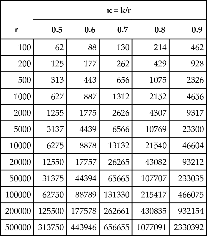
Regression using a varying-coefficients model for the expected values results in a fitted equation
ˆν=0.0277r(324)κ
![]()
which shows a (not unexpected) linear dependence on r, but an exponential relationship with κ. This demonstrates that as κ increases (i.e., as the proportion of distinct attractors in the sample increases) the expected number of attractors in the search space increases dramatically. The results for confidence intervals in Table 2 show that there will be considerable uncertainty for small samples (r < 10000, say. at least for relatively large κ), but of course, with larger samples, the estimate becomes more precise. The other noteworthy feature is the asymmetric nature of the intervals, reflecting a highly-skewed distribution for ˆν![]() . Finally, for large values of κ (> 0.95, say), it is not possible to use Eq. 5 at all, since the implied value of k when the + sign of Eq. 5 is taken exceeds r.
. Finally, for large values of κ (> 0.95, say), it is not possible to use Eq. 5 at all, since the implied value of k when the + sign of Eq. 5 is taken exceeds r.
Table 2
95% confidence intervals for v at some values of k/r and r. For example, if κ = 0.7 and r = 500, we are 95% confident that u lies between 581 and 745.
| r | κ = k/r | ||||
| 0.5 | 0.6 | 0.7 | 0.8 | 0.9 | |
| 100 | 53-73 | 72-110 | 101-176 | 153-331 | 288-1040 |
| 200 | 112-140 | 153-206 | 217-322 | 336-576 | 653-1539 |
| 500 | 292-337 | 404-488 | 581-745 | 917-1286 | 1842-3116 |
| 1000 | 596-660 | 830-950 | 1204-1436 | 1920-2437 | 3930-5680 |
| 2000 | 1210-1301 | 1693-1862 | 2470-2797 | 3969-4696 | 8244-10684 |
| 5000 | 3066-3210 | 4308-4575 | 6315-6831 | 10222-11368 | 21532-25357 |
| 10000 | 6174-6377 | 8692-9070 | 12775-13504 | 20756-22375 | 44051-49445 |
| 20000 | 12407-12694 | 17493-18027 | 25758-26788 | 41964-44252 | 89547-97165 |
| 50000 | 31148-31603 | 43975-44819 | 64857-66487 | 105925-109542 | 227163-239197 |
| 100000 | 62429-63072 | S8195-89388 | 130185-132490 | 212885-218000 | 457712-474726 |
| 200000 | 125046-125956 | 176737-178425 | 261039-264299 | 427244-434478 | 920270-944328 |
| 500000 | 313031-314470 | 442614-445283 | 654086-659240 | 1071398-1082835 | 2311519-2349554 |
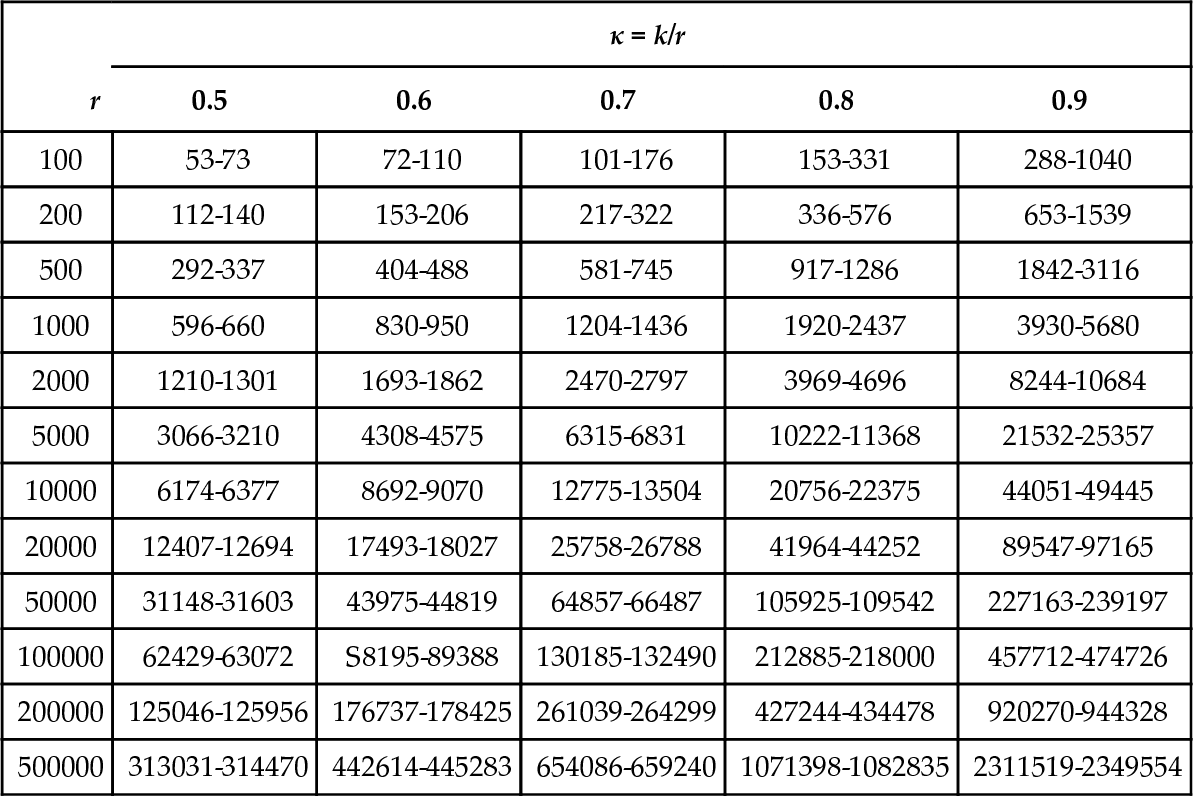
On the other hand, in cases where r is large relative to v, the ratio k/r may be very small, and care is needed in attempting to solve Eq. 2 numerically. In such cases, the best estimate of v is often simply k or k + 1. Likewise, the approximation in Eq. 3 is not suitable for small values of κ—in fact, simple numerical calculations show that unless κ > 0.55, Eq. 3 yields a value for v that is actually smaller than k, which is clearly impossible.
In practice this is likely to be irrelevant for most optimization problems—the interesting cases are those where we expect that κ > 0.7, say, and v will be much larger than r. Nevertheless, we now consider both issues—the cases of large and small κ.
3 FIRST REPETITION WAITING TIME DISTRIBUTION
As remarked above, in many cases v will be a very large number, as will be k—so it might be that every one of the attractors found is distinct unless r itself is quite large. Of course, if we find that k = r there will be no solution to Eq. 2. and all that we can say for certain is that there are at least k attractors. This outcome would be most unlikely, of course. One possibility is to keep sampling the set of all attractors until the first re-occurrence of a previously encountered attractor. Suppose this occurs on iteration T. We will call this the waiting time to the first repetition.
Proposition 2
The probability distribution of T is given by
P[T=t]=ν!(t−1)(ν−t+1)!vt2≤t≤ν+1orP[→T=t]=ν(ν−1)…(ν−t+2)(t−1)νt
The proof of this proposition again follows a straightforward combinatorial argument: the number of ways of choosing (t – 1) distinct objects from v (in any order) is (νt−1)(t−1)!![]() , while the total number of possible arrangements of v objects in (t – 1) trials is vt−1. The ratio of these quantities gives the probability that (t – 1) distinct attractors are encountered in (t – 1) trials. The probability that the tth trial encounters one of those attractors previously seen is (t – l)/v. Hence the result.
, while the total number of possible arrangements of v objects in (t – 1) trials is vt−1. The ratio of these quantities gives the probability that (t – 1) distinct attractors are encountered in (t – 1) trials. The probability that the tth trial encounters one of those attractors previously seen is (t – l)/v. Hence the result.
The mean of T is
E[T]=2ν+ν+1∑t=3t(t−1)ν!(ν−t+1)!νt
![]()
which seems to have no obvious closed-form solution. However, this and other statistics can in principle be computed for a given value of N using the obvious recurrence formulae
P[T=t+1]=tt−1ν−t+1νP[T=t]
![]()
(with P[T = 2] = 1/v) to calculate the probabilities. For large values of v this may take some time, and it is quicker to evaluate the median. Figure 1 shows the results of computations of median waiting time, and associated upper and lower quartiles, for a range of values of v.
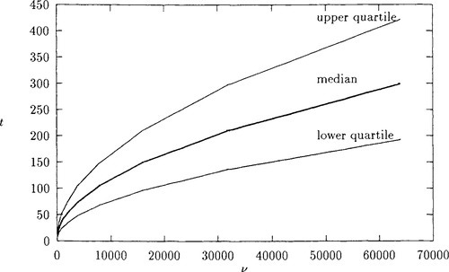
From this diagram it appears that the average waiting time is increasing as something like v0.5. A linear regression analysis confirmed that this is a plausible model, the actual relationship estimated over the range of values in the diagram being
tmed=0.673+1.25√ν
![]()
with a coefficient of determination (R2) of almost 100%.
3.1 Maximum likelihood estimation
For a single determination T = t the log-likelihood is
l(ν)=logν!+log(t−1)−log(ν−t+1)!−tlogν
and the first difference is
Δl=logν−log(ν−t+1)−t(logν−log(ν−1))
![]()
which gives an equation that is clearly a special case of Eq. 2
log(1−t−1ν)=tlog(1−1/ν)
Thus the numerical methods described in section 2.3 can also be used for this case. If we carry out multiple runs of the algorithm, so that we have m determinations (t1,…,tm), the generalization of the above is simply
m∑i=1log(1−ti−1ν)=log(1−1/ν)m∑i=1ti.
This can be simplified to
l(ν)=m∑i=1(ν∑k=ν−ti+2logk−tilogν)+termsnotinvolvingν
From this a direct line search algorithm can be devised for finding the maximum of l(v) and hence the maximum likelihood estimator of v. (Note that further algorithmic simplifications can be made by realising that many of the terms in the sum over k are repeated for all values of i—in fact all of them after k = v – tmin + 1 where tmin is the smallest value among the tt.) The author found that a golden section search based on this approach worked almost as well as the Newton-Raphson method used in section 2.3.
We can also find what appears to be a fairly good approximation, using natural logarithms in Eq. 6, and Stirling’s approximation
lnν!≈ln2π2+(ν+12)lnν−ν

Setting dl(ν)dν=0 gives the following, after some algebra:
ν=x2(1−x)+tln(1−x)

where x = (t – 1)/v. This can easily be iterated to a solution. (It is very easily handled in a spreadsheet, for example.) Again, if we have multiple determinations of T, the generalization is easy to obtain:
ν=−∑mt=1[xt2(1−xt)+ti]∑mi=1ln(1−xi).
Note that even when we exhaust our resources, and still we have k = r, we could use the techniques described above on the assumption that iteration r + 1 will provide the first re-occurrence. In this way, we could calculate a conservative estimate of v.
3.2 Further Approximations
Since we can expect x ![]() 1 in most interesting instances of optimization problems, it is possible to expand the right-hand side of Eq. 8 in powers of x, truncate, and solve the resulting equation for v. This produces
1 in most interesting instances of optimization problems, it is possible to expand the right-hand side of Eq. 8 in powers of x, truncate, and solve the resulting equation for v. This produces
ν(x+x22+x33+⋯)=x2+x22+x32+⋯+t
Truncating after the 1st term clearly fails to provide a sensible estimate, but truncating after the second-order term gives the following:
ν(x+x22)=x2+x22+t.
On substituting for x, and after some algebra, we find
2ν2−(t−1)(t−2)ν+(t−1)2=0,
![]()
and solving the quadratic for v (and taking the positive square root) leads to
ν*≈(t−1)(t−2)2,
which confirms the empirical observation in Fig. 1. In the case of multiple runs the quadratic is
av2+bv+c=0
![]()
with coefficients
a=2m,b=–(U2–3U1+2m),c=U2—2U1+m
![]()
where
Uk=m∑t=1(ti)k.
4 ESTIMATING THE NUMBER OF SAMPLES
We might expect that most of the time we will be faced with problems having large values of v (and thus of κ). However, some problem instances may have relatively small values, in which case we have a different but still interesting question: how long should we sample before we can reasonably be sure that all attractors have been found? We can model this situation as follows.
Suppose there are v attractors, and that we have already found k of them. The waiting time Wk for the (k + l)st attractor will have a geometric distribution
f(t|k)=ν−kν(kν)t−1
with expectation v/(v – k) and variance kv/(v — k)2. The overall waiting time will be
W=1+ν−1∑k=1Wk
and since these waiting times are independent, we can approximate the expectation and variance as follows:
E[W]=1+ν−1∑k=1νν−k=νν∑k=11k≈ν(lnν+γ)
where γ = 0.57721.. is Euler’s constant: and
V[W]=0+ν−1∑k=1kν(ν−k)2=ν2ν−1∑k=11k2−νν−1∑k=11k=ν2ζ(2)−ν(lnν−γ−1/ν)
where ζ(s)=∑∞1k−s is Riemann’s zeta function. The case s = 2 is a special case, for which ζ(2)=π2/6
![]() , so finally
, so finally
V[W]≈(νπ)26+1−v(lnv+γ)
![]()
Although both expressions are approximations, the errors are fairly small. The error in using Euler’s constant is already below 1% for v = 15, and while larger and slower to fall, the error in the infinite sum approximation drops below 2.5% for v = 25. Further, the errors are in opposite directions—one is a lower and the other an upper bound, so the net effect is likely to be unimportant.
We can use these estimates together with a Normal approximation to establish with probability a that the waiting time will exceed a given value:
W>ν(lnν−γ)+zα√(νπ)26+1−ν(lnν+γ).
where za is the appropriate standard Normal value. Finally, the right-hand side of the above expression can be inverted (numerically) to find a confidence limit on v. Table 3 gives some representative values, obtained very simply by using a spreadsheet equation solver.
Table 3
Table giving upper confidence limits for v at some representative values of r. For example, if we sample 2000 times and find 210 local optima, we can be 99% (but not 99.9%) confident that we have found them all.
| No. samples (r) | upper limit on v | |
| 99% | 99.9% | |
| 100 | 16 | 14 |
| 200 | 29 | 26 |
| 500 | 65 | 59 |
| 1000 | 120 | 109 |
| 2000 | 223 | 204 |
| 5000 | 511 | 468 |
| 10000 | 959 | 884 |
| 20000 | 1808 | 1673 |
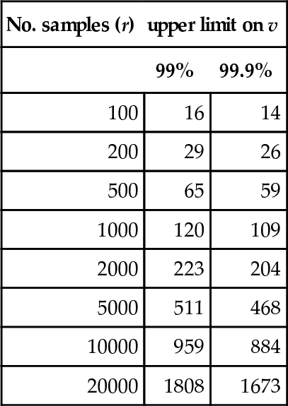
If the actual number of distinct local optima found in r samples is no more than the value given by such calculations, we can be confident (to approximately the degree specified) that we have found all the local optima. As already remarked, while the estimates of both mean and variance have small errors, they are unlikely to have a large influence on the degree of confidence. However, while the assumption of Normality is convenient, it is probably not well-founded: there is clearly a lower bound on the value of W, since it cannot be less than v, while the upper tail of the distribution may be very long. Thus, we should perhaps make do with Chebyshev’s inequality
Pr[|W−E[W]V[W]|≥c]≤1c2
which gives a less sharp, but still useful, confidence limit.
5 AN APPLICATION
In principle, this approach could be useful in providing some assurance of the quality of solutions obtained in the course of a heuristic search. Not only does it tell us something (although not everything) about the landscape, but at least tentatively, we now have a statistical way of assessing the amount of search that we need in order to find the global optimum with a reasonable probability.
It also gives us a means of comparing different representations and operators. For example, in the case of a GA, we could estimate the number of attractors resulting from the application of a GA, and compare this with what happens using a deterministic neighbourhood search using a bit flip operator, as a way of measuring the ‘improvement’ resulting from using a GA. (Of course, just looking at the numbers is not the only criterion—the quality of the respective solutions should also be taken into account.)
In (Reeves, 2000) it is shown that it is possible to generate sets of equivalent N K- landscapes—as introduced by (Kauffman, 1993); equivalent in the sense that all have the same epistasis variance, while having widely differing numbers of local optima with respect to a bit flip neighbourhood search. (The use of this operator implies that the underlying the landscape is based on the Hamming metric. Thus we shall call it the Hamming landscape.) However, how these landscapes compare with respect to a GA is not clear. Two NK-functions with N = 10,12 and K = 4 were chosen, representing those furthest apart in terms of numbers of Hamming landscape local optima. These are labelled ‘hard’ and ‘easy’ below. Each problem was solved repeatedly using a steady-state GA having the following parameters: population size 32, linear rank-based selection of parents, crossover was always performed (either one or two point), followed by mutation at a rate of either 0.05 or 0.10 per bit. One new offspring was produced at each iteration, and it replaced one of the worst 50% of the existing population. The run was terminated at convergence to an attractor.
At this point, we should explain what is meant by ‘convergence’. In the sense of (Vose, 1999), an attractor is a population, which does not necessarily coincide with a corner point of the simplex—i.e., it may not consist of multiple copies of a single string. Whenever mutation is involved, there is always the possibility of some variation, so detecting that an attractor (in the Vose sense) has been found is somewhat imprecise. As a reasonable heuristic, in these experiments it was defined as the situation when 90% of the population agreed about the allele at each locus. In order to guard against very long convergence times in the computer experiments, a termination criterion was also included in the code: that the run should be ended after 512 strings (a large fraction of the entire search space for these problems) had been evaluated. As a matter of fact, however, this criterion was never needed for the parameters tested, although with higher mutation rates and a softer selection pressure such a criterion might become necessary.
The numbers of attractors found on this basis in a sample of 100 replicate runs were counted and an estimate made using the methodology developed above. The results were as shown in Table 4. The numbers of local optima with respect to the neighbourhood search were obtained by exact counting using a version of Jones’s ‘reverse hill-climbing’ approach (Jones, 1995). However, it is not possible to compute the numbers of attractors exactly for a GA, even when the parameters are fixed, since there is so much randomization involved. What we estimate therefore is in some sense the number of the ‘most common’ attractors, ignoring possible pathological behaviour.
Table 4
A comparison of two equally ‘epistatic’ NK-landscapes with respect to NS and GAs for two different mutation rates and for 1-point and 2-point crossover.
| Landscape | # NS-local optima | # GA attractors | ||
| Mut | Rate | |||
| N = 10, K = 4 | xover | 0.10 | 0.05 | |
| ‘easy’ | 9 | 1 | 15 | 17 |
| 2 | 12 | 14 | ||
| ‘hard’ | 35 | 1 | 16 | 23 |
| 2 | 18 | 18 | ||
| N = 12, K = 4 | ||||
| ‘easy’ | 16 | 1 | 14 | 25 |
| 2 | 14 | 18 | ||
| ‘hard’ | 52 | 1 | 23 | 24 |
| 2 | 16 | 22 | ||
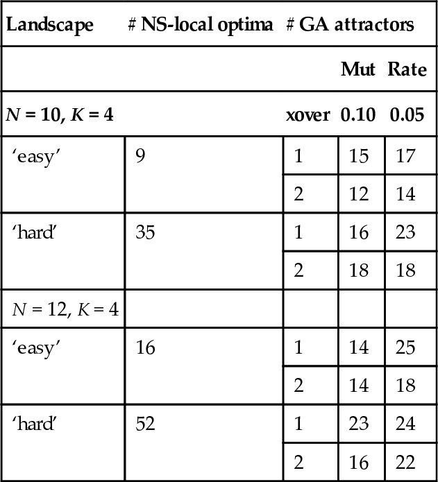
This is merely a small example, but even this demonstrates some interesting differences in the performances of the GAs. The number of GA attractors for the ‘easy’ landscapes is generally smaller (with a notable exception for the N = 12 case with mutation at 0.05) than for the ‘hard’ ones, and there does appear to be a difference between the 1-point and 2-point crossovers. We might also intuit that high mutation rates would imply fewer attractors, and this is evident in most cases (with the N = 12 case again an exception). It is also clear that just examining the NS landscape may not be adequate in predicting the performance of a GA. The number of attractors is clearly more than the number of NS-local optima in the ‘easy’ case, and seems likely to be fewer in the ‘hard’ case.
In some further experiments, a set of 35 equivalent NA’-functions (with N = 15, K = 4) was investigated; for each case a GA was run (as described above, with 1-point crossover and 0.10/bit mutation rate) for 100 independent trials. The number of attractors was estimated and compared with the (known) number of bit-flip local optima for each of the related landscapes. The correlation between the number of GA attractors and the number of Hamming local optima was 0.72, a statistically significant value. When the actual strings were compared, the set of GA attractors was almost always a subset of the Hamming local optima. Thus, although the landscapes are different in general, it seems that their fixed points tend to coincide, and despite the conceptual difference between deterministic point-based NS methods and stochastic population-based GAs, their respective landscapes seem to have similar properties.
Finally, the numbers of GA attractors was re-estimated using 500 independent runs instead of 100. In every case, the initial estimated number of attractors was exceeded, and although the numbers of attractors using 500 runs was well predicted by the numbers estimated using 100 runs (all fell within the initial 95% confidence interval), the correlation with the numbers of Hamming local optima was less strong (0.51 instead of 0.72). Now the set of attractors included points that were not Hamming local optima, so this reduction in correlation was not altogether a surprise. However, the ‘new’ attractors tended to be less fit than those found in the first 100 runs, and obviously they had a smaller attractive basin. This has some implications for the usefulness of the methodology that will be discussed in the next, final, section.
6 CONCLUSIONS AND FURTHER WORK
Several procedures have been presented for an empirical investigation of one aspect of a GA landscape. Previous approaches have not been able directly to answer the question of how many attractors there are, but the approach described here is able to estimate this quantity. Several practical questions of implementation have been reviewed, and an application has been made in order to demonstrate the methodology. The techniques described are not limited to GAs, but can in principle be applied to any heuristic search method.
There are some caveats that we should mention. Firstly, there is clearly a substantial computational burden in such investigations, and the size of the problem instance is clearly a factor in the feasibility of this approach. The number of samples needed may become infeasibly large as the size of the problem space increases.
Secondly, any estimate is useful only as long as the assumptions upon which it is based are valid. The fundamental assumption made above is that the attractors are isotropically distributed in the landscape, which implies that their basins of attraction are of more or less equal size. In fact, this is almost certainly not the case for many instances of NS landscapes. Such landscapes have been investigated empirically for such problems as the TSP, graph bisection and flowshop scheduling (Kauffman, 1993; Boese et al., 1994; Reeves, 1999b), and in many cases it is found that the local optima tend to be clustered in a ‘big valley’—closer to each other (and to the global optima) than a pair of randomly chosen points would be. Furthermore, the better optima tend to be closer to the global optima, and to have larger basins of attraction, than the poorer ones. Thus, optima found by repeated local searches are disproportionately likely to be these ‘more attractive’ (and hopefully fitter) ones. The number of local optima found by assuming an isotropic distribution is therefore likely to be an under-estimate of the true value. Nevertheless, we might hope that the statistical estimates would still be useful, as many of the local optima that we failed to find in a non-isotropic landscape would not (if the big valley conjecture holds) be very important anyway.
We do not know if similar patterns affect GA landscapes and attractors, but we have to recognize the possibility. Certainly, this is suggested by the analysis of the 35 equivalent NK-functions in the previous section. When the number of runs was extended from 100 to 500, several more attractors were found, more than had been estimated by the methods of the previous sections. These attractors seemed to have small basins, and to be less fit, so the remarks above relating to local optima seem to be echoed for the case of GA landscapes too.
In the applications above the effect of a non-isotropic distribution of attractors is probably not acute. When we compare the relative performance of different operators, for example, the effects of a non-isotropic distribution may apply in the same way to all of them. Also, on the empirical evidence of many fairly large studies of NS landscapes, and on the (admittedly much smaller) examples of GA landscapes investigated above, the attractors in the ‘tail’ of the distribution of basin sizes may be relatively unimportant. The assumption of approximate uniformity among the ones that we do care about is much more reasonable, and might mean that the estimates we obtain are fairly accurate, as long as we interpret them as referring to these ‘good’ attractors.
Nevertheless, if we wish to find still better estimates of the number of attractors, the effects of a non-uniform spread of attractors should be taken into account. A second paper that is currently in preparation will both examine the extent of the effect of the assumptions in the above analysis, and also explore stochastic models of non-isotropic landscapes.