
Local Search and High Precision Gray Codes: Convergence Results and Neighborhoods
Darrell Whitley [email protected]; Laura Barbulescu [email protected]; Jean-Paul Watson [email protected] Department of Computer Science, Colorado State University, Fort Collins, Colorado 80523 USA
Abstract
A proof is presented that shows how the neighborhood structure that is induced under a Gray Code representation repeats under shifting. Convergence proofs are also presented for steepest ascent using a local search bit climber and a Gray code representation: for unimodal 1-D functions and multimodal functions that are separable and unimodal in each dimension, the worst case number of steps needed to reach the global optimum is ![]() with a constant ≤ 2. We also show how changes in precision impact the Gray neighborhood. Finally, we also show how both the Gray and Binary neighborhoods are easily reachable from the Gray coded representation.
with a constant ≤ 2. We also show how changes in precision impact the Gray neighborhood. Finally, we also show how both the Gray and Binary neighborhoods are easily reachable from the Gray coded representation.
1 Introduction
A long-standing debate in the field of evolutionary algorithms involves the use of bit versus real-valued encodings for parameter optimization problems. The genetic algorithm community has largely emphasized bit representations. On the other hand, the evolution strategies (ES) community [10] [9] [10] [1] and, more recently, the evolutionary programming (EP) community [4] have emphasized the use of real-valued encodings. There are also application-oriented genetic algorithm researchers (e.g., [3]) who have argued for the use of real-valued representations.
Unfortunately, positions on both sides of the encoding debate are based almost entirely on empirical data. The trouble with purely empirical comparisons is that there are too many factors besides representation that can impact the interpretation of experimental results, such as the use of different genetic operators, or differences in experimental methodology. This work provides a better theoretical foundation for understanding the neighborhoods induced by a commonly used bit representation: Standard Binary Reflected Gray Codes.
One disadvantage of bit representations is that they generally do not offer the same precision as real-valued encodings. Often, genetic algorithms use 10 bits per parameter, while ES/EP approaches use full machine precision. On the one hand, different levels of precision can impact how accurately the global optimum is sampled, and can even change the apparent location of the optimum. Higher precision results in greater accuracy. But higher precision enlarges the search space, and conventional wisdom suggests that a smaller search space is generally an easier search problem. Yet, this intuition may be wrong for parameter optimization problems where the number of variables is fixed but the precision is not. This work examines how the search space changes as precision is increased when using bit encodings. In particular, we focus on how neighborhood connectivity changes and how the number of local optima can change as encoding precision is increased.
While our research is aimed at a very practical representation issue, this paper explores several theoretical questions related to the use of Gray codes, and high precision Gray codes in particular. These results have the potential to dramatically impact the use of evolutionary algorithms and local search methods which utilize bit representations.
We also present proofs which demonstrate that strong symmetries exist in the Hamming distance-1 neighborhood structure for Gray code representations. Given an L-bit encoding, we then prove that the worst-case convergence time (in terms of number of evaluations) to a global optimum is ![]() for any unimodal 1-dimensional function encoded using a reflected Gray code and a specialized form of steepest ascent local search under a Hamming distance-1 neighborhood. Under standard steepest ascent, the worst-case number of evaluations needed to reach a global optimum is
for any unimodal 1-dimensional function encoded using a reflected Gray code and a specialized form of steepest ascent local search under a Hamming distance-1 neighborhood. Under standard steepest ascent, the worst-case number of evaluations needed to reach a global optimum is ![]() for any unimodal 1-dimensional function. In both cases, the number of actual steps required to reach a global optimum is at most 2 L. This
for any unimodal 1-dimensional function. In both cases, the number of actual steps required to reach a global optimum is at most 2 L. This ![]() convergence time also holds for multidimensional problems when each dimension is unimodal and the intersection of the optima for each dimension leads to the global optimum. This includes problems such as the sphere function. In addition, we note some limitations of both Gray and Binary neighborhoods; we then prove that the standard Binary neighborhood is easily accessible from Gray space using a special neighborhood (or mutation) operator.
convergence time also holds for multidimensional problems when each dimension is unimodal and the intersection of the optima for each dimension leads to the global optimum. This includes problems such as the sphere function. In addition, we note some limitations of both Gray and Binary neighborhoods; we then prove that the standard Binary neighborhood is easily accessible from Gray space using a special neighborhood (or mutation) operator.
2 Local Optima, Problem Complexity, and Representation
To compare representations, it is essential to have a measure of problem complexity. The complexity measure we propose is the number of local optima in the neighborhood search space. There is evidence that the number of local optima is a relatively useful measure of problem complexity, that it impacts problem complexity, and relates to other measures such as schema fitness and Walsh coefficients [8] for problems using bit representations.
Suppose we have N unique points in our search space, each with k neighbors, and a search operator that evaluates all k neighboring points before selecting its next move; similar results hold for most non-unique sets of values. A point is considered a local optimum from a steepest ascent perspective if its evaluation is better than all of its k-neighbors. We can sort these N points to create an ordinal ranking, R = r1, r2,…, rN, where r1 is the global optimum of the search space and rN is the worst point in the space. Using R, we can compute the probability P(i) that a point ranked in the i-th position in R is a local optimum under an arbitrary representation, given a neighborhood of size k:
Proof:
For any point in the search space, there are  possible sets of neighbors for that point. If the point is ranked in position r1, then there are
 ![]() sets of neighbors that do not contain a point of higher evaluation than the point r1. Therefore, the point ranked in position r1 will always be a local optimum under all representations of the function. In the general case, a point in position r1, has only
sets of neighbors that do not contain a point of higher evaluation than the point r1. Therefore, the point ranked in position r1 will always be a local optimum under all representations of the function. In the general case, a point in position r1, has only ![]() sets of neighbors that do not contain a point of higher evaluation than the point ri. Therefore the probability that the point in position ri remains a local optimum under an arbitrary representation is
sets of neighbors that do not contain a point of higher evaluation than the point ri. Therefore the probability that the point in position ri remains a local optimum under an arbitrary representation is ![]() .
. ![]()
This proof also appears in an IMA workshop paper [7]. These probabilities enable us to count the expected number of local optima that should occur in any function of size N. The formula for computing the expected number of times a particular point will be a local optimum is simply N! × P(i). Therefore the expected number of optima over the set of all representations is:
Rana and Whitley [7] show that to find the expected number of local optima for a single representation instance, we divide ε(N, k) by N!, which yields:
This result leads to the following general observation: in expectation, if we increase neighborhood size we decrease the number of local optima in the induced search space. Can we leverage this idea when constructing bit representations? In particular, can we construct bit representations that increase neighborhood size while also bounding or decreasing the number of local optima?
3 Gray and Binary Representations
Another much-debated issue in the evolutionary algorithms community is the relative merit of Gray code versus Standard Binary code bit representations. Generally, “Gray code” refers to Standard Binary Reflected Gray code [2]. In general, a Gray code is any bit encoding where adjacent integers are also Hamming distance-1 neighbors in the bit space. There are exponentially many Gray codes with respect to bit length L. Over all possible discrete functions that can be mapped onto bit strings, the space of all Gray codes and the space of all Binary representations are identical. Therefore, a “No Free Lunch” result must hold [13] [5]. If we apply all possible search algorithms to Gray coded representations of all possible functions and we apply all possible search algorithms to Binary representations of all possible functions, the behavior of the algorithms must be identical for the two sets of representations since the set of all possible Gray coded and the set of all Binary coded functions are identical [11].
The empirical evidence suggests that Gray codes are usually superior to Binary encodings for practical optimization problems. It has long been known that Gray codes remove the Hamming Cliffs induced by the Standard Binary code, where adjacent integers are represented by complementary bit strings: e.g., 7 and 8 encoded as 0111 and 1000. Whitley et al. [12] note that every Gray code must preserve the connectivity of the original real-valued functions (subject to the selected discretization). Further, because of the increased neighborhood size, Gray codes induce additional connectivity which can potentially ‘collapse’ optima in the real-valued function. Therefore, for every parameter optimization problem, the number of optima in the Gray coded space must be less than or equal to the number of optima in the original real-valued function. Binary encodings offer no such guarantees. Binary encodings destroy half of the connectivity of the original real-valued function; thus, given a large basin of attraction with a globally competitive local optimum, most of the (non-locally optimal) points near the optimum of that basin become new local optima under a Binary encoding.
Recently, we proved that Binary encodings work better on average than Gray encodings on “worst case” problems [11]; a “worst case” function is such that when interpreted as a 1-D function, alternating points in the search space are local optima. “Better” means that the representation induces fewer local optima. (There is a definitional error in this proof; it does not impact “wrapping” functions, but does impact the definition of a worst case function for “non-wrapping” functions. See Appendix 1 for details and a correction.) A corollary to this result is that Gray codes on average induce fewer optima than Binary codes for all remaining functions. For small (enumerable) search spaces, it can also be proven that in general Gray codes are superior to Binary for the majority of functions with bounded complexity. A function with “lower complexity” in this case has fewer optima in real space. We use these theoretical results, as well as the empirical evidence to argue for the use of Gray codes.
But to be comparable to real-valued representations, bit representations must use higher precision. Higher precision can allow one to get “closer” to an optimum, and also creates higher connectivity around the optimum. But what happens when we use higher precision Gray codes?
We first establish some basic properties of Gray neighborhoods. We will assume that we are working with a 1-dimensional function, but results generally apply to the decoding of individual parameters.
4 Properties of the Reflected Gray Space
We begin by asking what happens when a function is “shifted.” Since we are working with bit representations, we assume that a decoder function converts bits to integers, and finally to real space. Shifting occurs after the bits have been converted to integers, but before the integers are mapped to real values. If there are L bits then we may add any integer between 0 and 2L − 1 (mod 2L). The only effect of this operator is to shift which bit patterns are associated with which real values in the input domain. Also note the resulting representation is still a Gray code under any shift [6].
What happens when one shifts by 2L − 1? Under Binary, such a shift just flips the first bit, and the Hamming distance-1 neighborhood is unchanged. A reflected Gray code is a symmetric reflection. Shifting therefore also flips the leading bit of each string, but it also reverses the order of the mapping of the function values to strings in each half of the space. However, since the Gray code is a symmetric reflection, again the Hamming distance-1 neighborhood does not change. This will be proven more formally.
It follows that every shift from i = 0 to 2 L ‒ 1 – 1 is identical to the corresponding shift at j = 2 L − 1 + i. We next prove that shifting by 2 L − 2 will not change the neighborhood structure; in general, shifting by 2 L ‒ k will change exactly k – 2 neighbors.
Theorem 1
For any Gray encoding, shifting by 2 L − kwhere 2 ≤ k ≤ L will result in a change of exactly k – 2 neighbors for any point m the search space.
Proof: Consider an arbitrary Gray code, and k ≥ 2. Divide the 2L points in the search space into 2k continuous blocks of equal size, starting from the element labeled 0. Each block contains exactly 2L − k elements corresponding to bit strings or integers (see Figure 1a). Consider an arbitrary block X and arbitrary element with label P within X. Exactly L – k neighbors of P are contained in X. The periodicity of both Binary and Gray bit encodings ensures that the L – k neighbors of P in X do not change when shifting by 2L − k. Two of the remaining k neighbors are contained in the blocks preceding and following X, respectively. Since the adjacency between blocks does not change under shifting, the two neighbors in the adjacent blocks must stay the same.

The remaining k – 2 neighbors are contained in blocks that are not adjacent to X. We prove that the rest of these k – 2 neighbors change. Consider a block Y that contains a neighbor of P. For every Reflected Gray code there is a reflection point exactly halfway between any pair of neighbors. For all neighbors outside of block X which are not contained in the adjacent blocks, the reflection points must be separated by more than 2L − k positions. Shifting X by 2L − k will move it closer to the reflection point, while Y is moved exactly 2L − k positions farther away from the reflection point (see Figure 1b). Point P in X must now have a new neighbor (also 2 L − k closer to the reflection point) in the block Z. If the reflection point between X and Z is at location R, then for the previous neighbor in Y to still be a neighbor of P in X it must have a reflection point at exactly R + 2L − k. This is impossible since for all neighbors outside of block X which are not contained in the adjacent blocks, the reflection points must be separated by more than 2L − k positions. A similar argument goes for the case when shifting by 2L − k moves X farther away from the reflection point (while Y is moved closer). Thus, none of the previous k – 2 neighbors are neighbors after shifting by 2L − k.
4.1 High Precision Gray Code and Longest Path Problems
We know that a Gray code preserves the connectivity of the real-valued space. If we think about search moving along the surface of the real-valued functions, then increased precision could cause a problem. The distance from any point in the search space and the global optimum might grow exponentially as precision is increased. If we must step from one neighbor to the next, then as we increase the number of bits, L, used to encode the problem, the distance along this adjacent-neighbor path grows exponentially long as a function of L. On the other hand, we know that connectivity in a hypercube of dimension L is such that no two points are more than L moves away from one another. This lead us to ask what happens when we increase the precision for Gray coded unimodal functions? We prove that the number of steps leading to the optimum is O(L).
4.2 Convergence Analysis for Unimodal and Sphere Functions
Consider any unimodal real-valued 1-dimensional function. Steepest ascent local search using the L-bit Hamming distance-1 neighborhood of any Reflected Gray-code representation of any unimodal real-valued function will converge to the globcil optimum after at most 2 L steps or moves in the search space.
Lemma 1
For any 1-dimensional unimodal real-valued function, steepest ascent local search using the L-bit Hamming distance-1 neighborhood of any Reflected Gray-code representation will converge to the global optimum after at most 2 L steps.
Proof: The proof assumes that all points in the search space have unique evaluations (to prevent search from being stuck on flat spots). We have already shown that for any Gray code representation shifting by 2L−2 does not change the structure of the search space. We can thus break the search space into four quadrants. This means we can assume the current point, P from which we are searching can be located in any quadrant, and the neighborhood structure is identical when P is shifted to the same position in any other quadrant of the search space.
Consider the following set of points: {a, N, b, c, P, c’, b’, N’ a’, x, Y, z}. The points {N, P, N’, Y} are located in the four quadrants and for any reflected Gray code 2 adjacent points in the sequence N, P, N’, Y, N are neighbors. Let points a and b be neighbors in the same quadrant as N, with a to the left and b to the right. The same holds for subsets {c, P, c’} {b’, N’, a’} and {x, Y, z} as shown in the following figure. The quadrants are labeled Ql, Q2, Q3 and Q4. Neighbors are connected by dashed lines.
Let P be the current position of the search. P has neighbors c, c’, N, and N’. The neighbors c and c’ are in the same quadrant as P, but N and N’ must be in adjacent quadrants of the space due to the reflected symmetry of Gray code. Y is in a position symmetric to N and reachable in 2 moves from P.
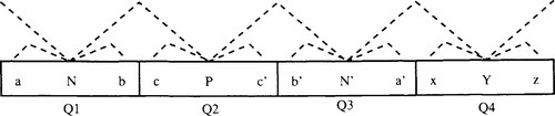
We now can decompose this problem into a series of cases. For any set of three points {w,x,y}, if we know that w > x < y then we know that a minimum, and hence the global minimum, must lie between w and y. (Note we use the same symbol to represent a point and its evaluation.) In this way, each case either eliminates at least half of the search space from further consideration, or leads to at most 2 moves to a neighbor from which it is possible to eliminate at least half of the search space. The only moves that are considered are those that change from one quadrant to another. (“In quadrant” moves can be considered as part of the next move.)
| POSITION | CASE | MOVE | QUADRANT TO ELIMINATE | ||
| P | C > P < c’ | none | Q1, | Q3, | Q4 |
| P | N > c < P | none | Q3, | Q4 | |
| P | P > c’ < N’ | none | Q1, | Q4 | |
| P | N’ > N < c | goto N | |||
| P | c’ > N’ < N | goto N’ | |||
| N | A > N < b | None | Q2, | Q3, | Q4 |
| N | Y > a < N | none | Q2, | Q3 | |
| N | N > b < c | none | Q3, | Q4 | |
| N | N > Y < N’ | goto Y | |||
| Y | X > Y < z | none | Q1, | Q2, | Q3 |
| Y | N’ > x < Y | none | Q1, | Q2 | |
| Y | Y > z < N | none | Q2, | Q3 | |
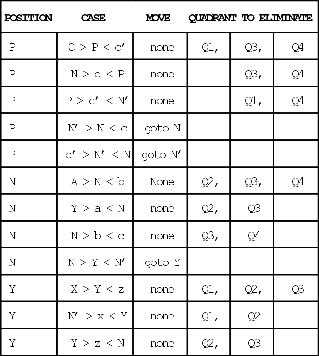
The cases for N’ are a symmetric reflection of the cases for N. There are no other cases. Thus after 2 moves it is always possible to reduce the search space by at least half. Furthermore the remaining quadrants are always adjacent (which is true by inspection).
After discarding half of the search space, we can treat the space as having been reduced by 1 dimension in Hamming Space. This reduction in the dimensionality can be recursively applied until L = 2. For L = 2 the search space is reduced to four points (one of which is the optimum) and it takes at most two moves to go to the optimum. By summation, it follows that it takes at most 2 L moves to go from any point in the space to the optimum.
If the optimum can be reached after at most 2 L moves, each move normally requires L – 1 evaluations under steepest ascent. But if the function is unimodal we only need to evaluate four critical neighbors that are used in the preceding proof. Therefore
Theorem 2
For any unimodal real-valued function, there exists a special form of steepest ascent local search using the L-bit Hamming distance-1 neighborhood of any Reflected Gray-code representation that will converge to the global optimum after at most![]() evaluations.
evaluations.
Proof: The result follows directly from the proof of Lemma 1.
4.3 Multi-parameter Problems and Sphere Functions
The proofs only deal with 1 dimensional functions. However, every multi-parameter separable function can be viewed as a composition of real-valued subfunctions. If each real-valued sub-function is unimodal and encoded with at most l bits, a specialized form of steepest ascent Hamming distance-1 local search using any Reflected Gray-code representation will converge to the global optimum after at most ![]() steps in each dimension. If there are Q dimensions and exactly I bits per dimension, note that Ql = L, and the overall convergence is still bounded by
steps in each dimension. If there are Q dimensions and exactly I bits per dimension, note that Ql = L, and the overall convergence is still bounded by ![]() . It also follows that
. It also follows that
Theorem 3
Consider the sphere function, ![]() denotes the minimum. For this sphere function, steepest ascent local search using the L-bit Hamming distance-1 neighborhood of any Reflected Gray-code representation will converge to the global optimum after at most
denotes the minimum. For this sphere function, steepest ascent local search using the L-bit Hamming distance-1 neighborhood of any Reflected Gray-code representation will converge to the global optimum after at most![]() steps.
steps.
4.4 The Empirical Data
The proof obviously shows that regular steepest ascent, where all L neighbors are checked, will converge in ![]() steps and
steps and ![]() total evaluations. A set of experiments with different unimodal sphere functions encoded using a varying number of bits shows behavior exactly consistent with the proof. The number of steps of steepest ascent local search needed to reach the optimum is linear with respect to string length. This is shown in Figure 2. This figure also shows that the number of evaluations used by regular steepest ascent is order
total evaluations. A set of experiments with different unimodal sphere functions encoded using a varying number of bits shows behavior exactly consistent with the proof. The number of steps of steepest ascent local search needed to reach the optimum is linear with respect to string length. This is shown in Figure 2. This figure also shows that the number of evaluations used by regular steepest ascent is order ![]() with respect to string length.
with respect to string length.

But what about next ascent? In the best case, next ascent will pick exactly the same neighbors as those selected under steepest ascent, and the number of steps needed to reach the optimum is ![]() . However, in the worst case an adjacent point in real space is chosen at each move and thus the number of steps needed to reach the optimum is
. However, in the worst case an adjacent point in real space is chosen at each move and thus the number of steps needed to reach the optimum is ![]() . The linear-time best case and exponential-time worst case makes it a little less obvious what happens on average. The advantage of next ascent of course, is that there can be multiple improving moves found by the time that L neighborhoods have been evaluated. Informally, what are the odds that none of the improving moves which are found are long jumps in the search space? If, for example, one found a best possible move and a worst possible move after evaluating L neighborhoods, the convergence time is still closer to the
. The linear-time best case and exponential-time worst case makes it a little less obvious what happens on average. The advantage of next ascent of course, is that there can be multiple improving moves found by the time that L neighborhoods have been evaluated. Informally, what are the odds that none of the improving moves which are found are long jumps in the search space? If, for example, one found a best possible move and a worst possible move after evaluating L neighborhoods, the convergence time is still closer to the ![]() steps and
steps and ![]() evaluations associated with blind steepest ascent. The empirical data seems to suggest that the average case is similar to the best case. The rightmost graph in Figure 2 shows that the empirical behavior of Random Bit Climbing appears to be bound by L log(L) on average. This is in fact better than the L2 behavior that characterizes the number of evaluations required by steepest ascent. The variance is so small in both cases as to be impossible to be seen on the graphs shown here.
evaluations associated with blind steepest ascent. The empirical data seems to suggest that the average case is similar to the best case. The rightmost graph in Figure 2 shows that the empirical behavior of Random Bit Climbing appears to be bound by L log(L) on average. This is in fact better than the L2 behavior that characterizes the number of evaluations required by steepest ascent. The variance is so small in both cases as to be impossible to be seen on the graphs shown here.
We used Davis’s Random Bit Climber (RBC) as our next ascent algorithm. RBC randomized the order in which the bits are checked. After every bit has been tested once, the order in which the bits are tested is again randomized. This randomization may be important in avoiding worst case behavior.
5 High Precision Gray Codes and Local Optima
Our results on the expected number of optima under a neighborhood search operator of size k confirm the intuitive notion that, in expectation, larger neighborhood sizes generally result in fewer optima. One way to increase the neighborhood size for bit-encoded parameter optimization problems is to increase the encoding precision of each parameter. This initially seems counter-intuitive, because it also increases the size of the search space. A 10 parameter optimization problem with a 10-bit encoding results in a search space of 2100 points, while a 20-bit encoding results in a search space of 2200 points. Generally, a smaller search space is assumed to be “easier” than a larger search space. But is this true?
Consider a parameter X with bounds Xlb and Xub From an L-bit representation, an integer y is produced by the standard Binary or Gray decoding process. This integer is then mapped onto an element ![]() . We refer to y as an integer point and x as the corresponding domain point.
. We refer to y as an integer point and x as the corresponding domain point.
We begin with an illustrative example. Let Xlb = 0 and Xub = 31, and consider an L-bit Gray encoding of X, with 5 ≤ L ≤ 10. Table 1 shows the L domain neighbors of the domain point nearest to 4.0; for reasons discussed below, 4.0 may not be exactly representable under an arbitrary L-bit encoding. Under a 5-bit Gray encoding, the integer neighbors of y5 = 4 are 3, 5, 7, 11, and 27, as shown. And because of the domain bounds, these integers are also the domain neighbors of the point x = 4.0.
Table 1
Neighbors of the point nearest to x = 4.0 under a Gray encoding, 5 ≤ L ≤ 10.
| L | n ~ 3 | n introduced by increases in precision | n ~ 5 | n ~ 7 | n ~ 11 | n ~ 27 | ||||
| 5 | 3.000 | 5.000 | 7.000 | 11.000 | 27.000 | |||||
| 6 | 3.444 | 4.429 | 5.413 | 7.381 | 11.318 | 27.064 | ||||
| 7 | 3.661 | 4.149 | 4.638 | 5.614 | 7.567 | 11.472 | 27.095 | |||
| 8 | 3.647 | 3.890 | 4.133 | 4.619 | 5.592 | 7.527 | 11.428 | 26.988 | ||
| 9 | 3.701 | 3.943 | 4.065 | 4.186 | 4.671 | 5.642 | 7.583 | 11.466 | 26.996 | |
| 10 | 3.727 | 3.969 | 4.030 | 4.091 | 4.212 | 4.697 | 5.667 | 7.606 | 11.485 | 27.000 |
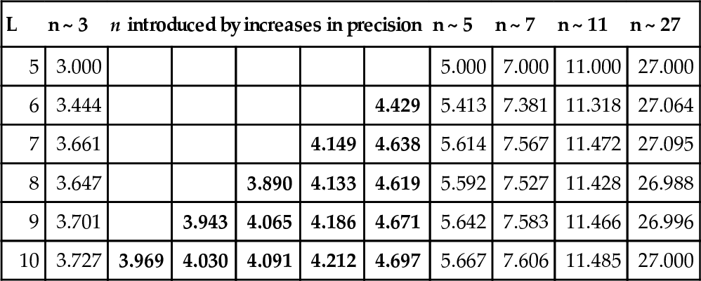
Table 1 shows that increasing the precision can influence the neighborhood structure under Gray encodings. The point of reference is x and its neighbors are n.
Two things are important about the pattern established in Table 1. First, as precision is increased, the set of neighbors when L = 5 continue to be represented by neighbors near to the original set of neighbors. Thus, all of the original neighbors are approximately sampled at higher precision. Second, note that when L = 5, the nearest neighbor of x = 4.0 are n = 3.0 and n = 5.0. All new neighbors of x fall between 3.0 and 5.0.
This observation suggests that we might wish to consider the stability of the original set of neighborhoods as we increase precision. And it also suggests that higher precision does not necessarily change the number of optima, and thus, using higher precision does not hurt or help when “number of local optima” is used as a measure of complexity.
Note our observation makes strong assumptions. Table 1 shows that in fact there is considerable instability in the position of neighbors 3–11, there is slight instability in the domain neighbor 27. A contributing cause, albeit minor, to the instability of the domain neighbors is due to the following
Theorem 4
Let Xlb, and Xub denote the lower and upper bounds on the domain of a parameter X. Consider bit encodings (Gray or Binary) of X with precisions L and L + 1. Define![]() for some decoded integer yL, 0 ≤ yL ≤ 2L – 1; zL is a point in the domain of X representable under an L-bit encoding. Then there exists no yL + L (except for 0 and 2L + 1 – 1) such that zL = zl + 1 - i.e., identical points are not representable under bit encoding after changing the precision by one 1.
for some decoded integer yL, 0 ≤ yL ≤ 2L – 1; zL is a point in the domain of X representable under an L-bit encoding. Then there exists no yL + L (except for 0 and 2L + 1 – 1) such that zL = zl + 1 - i.e., identical points are not representable under bit encoding after changing the precision by one 1.
Proof: Suppose that there exists yL + 1 such that zL = zL + 1 Using the definition for zl we obtain:
![]()
The equation above implies that (2L – 1) evenly divides 2LyL, which is a contradiction if yL + 1 ≠ 0 and yL + 1 ≠ 2L + 1 – 1! Indeed, (2L – 1) does not evenly divide 2L. The only 2 values of yL which are evenly divided by (2L – 1) are 0 and (2L – 1). But if yL = 2L – 1, then zl = zl + 1 = Xub, and therefore yL + 1 = 2L + 1 - 1 (value already accounted for by the theorem). Similarly, if yL = 0 then yL + 1 = 0.
For example, consider a 10-bit encoding of a parameter X with Xlb, = 0 and Xub, = 16 The decoded integer 512 maps to the domain value 8.993157. Increasing the precision to 11 bits, the nearest domain values are represented by the integers 1150 (8.988764) and 1151 (8.996580). While the difference is relatively minor (~ 0.004), altering the precision nonetheless changes the representable domain values. Further, this change is independent of the choice of Gray or Binary bit encodings. However note that this proof does not preclude recycling of point at different precisions.Table 1 shows that the same points can be resampled when the precision changes by more than 1 bit. Table 1 also shows that the change in distance from some fixed reference point does not change monotonically as precision is increased.
We can generate examples which prove that it is possible for minor changes in precision to either increase or decrease the number of optima which exists in Hamming Space due to small shifts in the locations of some “original” set of neighbors. Cases exists where two optima with similar evaluation exist at one level of precision in Gray space, and then collapse at higher precision. In addition, two optima in real space that were previously collapsed in Gray space at lower precision can again become separate optima in Gray space at higher precision. Nevertheless, the creation or collapse of an optimum under higher precision appears to be a symmetric process-and we conjecture that in expectation, the creation and collapse of optima will be equal and that no change in the total number of optima would result.
Any remaining instability in the domain neighbors due to increases in precision must be explainable by changes in the neighborhood connectivity patterns. To characterize such changes, we divide the domain of a parameter X into 4 quadrants, denoted Q1 – Q4. Under both Gray and Binary encodings, a point in Q1 has a neighbor in Q2. Under a Gray code, the point in Q1 has a neighbor in Q4, and under Binary the same point has a neighbor in Q3. We can also “discard” Q3 and Q4 under both Binary and Gray encodings by discarding the first 1-bit. We can then cut the reduced space into 4 quadrants and the same connectivity pattern holds. (This connectivity pattern is also shown in Figures 3 and 4.)

First, we can show that increases in the precision fail to alter the location of neighbors from the quadrant viewpoint:
Theorem 5
Consider the decoded integer yL under an L-bit encoding, L ≥ 2. Increasing the precision to L + 1 yields yL + 1 = 2 yL. Let![]() represent the set of quadrants in which neighbors of yL reside. Then
represent the set of quadrants in which neighbors of yL reside. Then![]()
Proof: For the trivial case yL = yL + 1 = 0, the theorem is obviously true.
Consider yl ≠ 0, and zL the domain point corresponding to yL. Then, ![]() is the domain point corresponding to yL + 1, then similarly:
is the domain point corresponding to yL + 1, then similarly: ![]() . We will prove that zL and zL + 1 reside in the same quadrant, this being equivalent to
. We will prove that zL and zL + 1 reside in the same quadrant, this being equivalent to![]() .
.
In the real-valued domain, if zL resides in the qth quadrant (where q = 0..3), then the following inequalities are satisfied:
First, we compute the difference between zL and zL + 1:
Note that the differencr is positive;therefore zL + 1 < zL.
Let z′Lbe the domain point corresponding to yL – 1. Then:

Since ![]() , using (5) and (6), we can infer:
, using (5) and (6), we can infer:
![]()
If zl is notthe first point sampled in the qth quadrant by the L bit encoding, then z′Lmust also be in the same quadrant with zl Therefore, from the above inequality it results that zl + 1 must be in the same quadrant with zl and z′L.
Consider the case when zl is the first point sampled in the qth quadrant by the L bit encoding. Since the yL = 0 case was already considered, q = 1..3.
Suppose that zL + 1 is not in the same quadrant with zL This means that the distance between zL + 1 and zL is larger than the distance from zL to the starting point (in the real domain) of the qth quadrant:
But, from (4):
Using (7) and (8), the difference between the two bounds discovered for yL is:
We distinguish 3 cases:
Case 1: q = 1
In this case q(2L – 1) is an odd number. Therefore, there exists an integer number p such that q(2L – 1) = 4p + 1 or q(2L – 1) = 4p + 3. Using (7), (8),and (9), we obtain:
or
(10), (11) can not be satisfied for any integer yL.
Case 2: q = 2
In this case  is an odd number. Therefore, there exists an integer number p such that
 ![]() . This implies:
. This implies:
Again, Case 2 (12) can not be satisfied for any integer yL.
Case 3: q = 3
As for case 1, q(2L – 1) is an odd number. However, there exists no integer p such that q(2l – 1) = 4p + 3. Indeed, suppose there exists an integer p such that 3(2L – 1) = 4p + 3.
This implies 2L−1 = (2/3)p + 1, where the right hand side of the equality must be integer, and therefore is odd. But 2L−1 is an even number. The contradiction obtained confirms that for no integer p, q(2L – 1) = 4p + 3. The only possibility left to express q(2L – 1) as an odd number is: q(2L – 1) = 4p + 1 where p is integer. For yL this implies:
It is clear that there exists no integer yL satisfying (13).
The contradictions obtained for the three possible values of q resulted from the assumption that zL + 1 is not in the same quadrant with zL. Thus, we proved by contradiction that zL and zL + 1 reside in the same quadrant.
Note that yL and yL + 1 are the decoded integers roughly corresponding to the same domain point (Theorem 4 prevents the exact correspondence to the same domain point). Theorem 5 establishes that increasing precision cannot change the quadrants sampled by the neighbors of a yL, but it says nothing about how the relative densities of those neighbors change in the various quadrants, or how the neighbors can shift positions within quadrants.
To explore the question of neighbor density, we consider an L-bit encoding (Gray or Binary) and an integer yL – 2 in a quadrant QyL – 2. There are L – 2 neighbors of yL – 2 in quadrant QyL – 2, and exactly one in two of the three remaining quadrants (Qy–adj–left and Qy–adj–right).
Next, we increase the precision by one to L + 1. Here, L – 2 neighbors of yL - 2 are compressed into ![]() of the domain, instead of
of the domain, instead of ![]() under the L-bit encoding. The remaining 3 neighbors are allocated as follows: exactly one in two of the remaining three new quadrants (Qy_adj_left and Qy_adj_right), and an additional neighbor in the quadrant QyL–2. Because of this compression, we find an increased density of neighbors near xL–2 as the precision is increased. In summary:
under the L-bit encoding. The remaining 3 neighbors are allocated as follows: exactly one in two of the remaining three new quadrants (Qy_adj_left and Qy_adj_right), and an additional neighbor in the quadrant QyL–2. Because of this compression, we find an increased density of neighbors near xL–2 as the precision is increased. In summary:
This observation is imprecise because the position of y also moves with the increased precision. This is clearly shown in Table 1. In addition to increased density, we see a ‘migration’ of domain neighbors within quadrants. Examining Table 1, we see that 3.0 under a 5-bit encoding migrates toward 3.7273 under a 10-bit encoding, and the migration is more than can be accounted for by Theorem 4. Consider a 4-bit Gray code and the integer 4, which has neighbors 3, 5, 7, and 11, and a corresponding domain point d4. Next, increase the precision to 5 bits. Now the domain point nearest to 4.0, subject to Theorem 4, is produced by the integer 8, with neighbors 7, 9, 11, 15, and 23. Since we have roughly doubled the precision, these neighbors correspond roughly to 3.5, 4.5, 5.5, 7.5, and 11.5, respectively, for the integer 4.
6 Combining Gray and Binary Neighborhoods
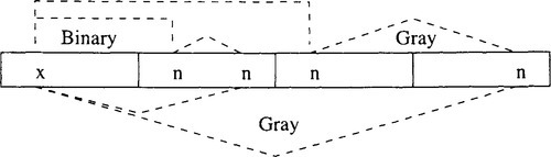
The “Quadrant” decomposition used previously in this paper also provides a helpful way to visualize connectivity bias in the Gray and Binary neighborhoods. Figure 3 illustrates That Binary and Gray neighbors reside in disjunct and complementary portions of the search space. We construct Figure 3 using our prior strategy of shifting any point of interest, x, to the first quadrant. Again, this can be done without changing the neighborhood structure of the space, x has exactly one Binary neighbor in the upper half of the space, in quadrant 3. Also, x has exactly one Gray neighbor in the upper half of the space, in quadrant 4. We recursively identify in the same way the location of the remaining Binary and Gray neighbors of x. First, we can discard quadrants 3 and 4 and consider the lowerdimensional problem. We then repeat the process of shifting the point of interest to the new lower-dimensional first quadrant. The lower dimensional neighborhood is unchanged.
Figure 3 shows how Gray and Binary codes connect x (via a Hamming distance-1 neighborhood) to complementary, disjoint portions of the search space. However, Figure 4 shows that the Hamming distance-1 neighbors under Binary are Hamming distance 2 neighbors in Gray space. Thus it is possible to construct a neighborhood of 2L – 1 points that include both the Binary and Gray neighbors. The goal of constructing such a neighborhood is to reduce the complementary bias which exists in the Gray and Binary neighborhood structures.
We will show that flipping single bits accesses the Gray neighborhood and that flipping pairs of adjacent bits accesses the Binary neighborhood. Consider the following bit vector B as a binary string. Assume strings are numbered from right to left starting at zero: B = Bl – 1, …, B1, B0. In particular we are interested in the bit Bi. Now convert B to a Gray code using exclusive-or. This results in the following construction
![]()
Now consider what happens when bit Bi is flipped, where 1 ≤ i ≤ l – 1. G changes at exactly two locations. Thus, we can access the Gray neighborhood by flipping individual bits and the Binary neighborhood by flipping adjacent pairs of bits. By combining Binary and Gray neighborhoods, we can never do worse than the original Gray space in terms of number of local optima which exist. To access these neighbors in a genetic algorithm, we would use a special mutation operator that flips adjacent pairs of bits.
7 Conclusions
We have presented four theoretical results which provide a better understanding of one of the most commonly used bit encodings: the family of Gray code representations. First, we showed that shifting the search space by 2L – 2 does not change the Gray code Hamming distance-1 neighborhood. Second, we showed that for any unimodal, 1dimensional function encoded using a reflected L-bit Gray code, steepest-ascent local search under a Hamming distance-1 neighborhood requires only ![]() steps for convergence to the global optimum, in the worst case. We showed that this result also holds for multidimensional separable functions. Third, we demonstrated how increasing the precision of the encoding impacts on the structure of the search space. Finally, we show that there exists a complementary bias in the Gray and Binary neighborhood structures. To eliminate this bias, a new neighborhood can be constructed by combining Gray and Binary neighborhood structures.
steps for convergence to the global optimum, in the worst case. We showed that this result also holds for multidimensional separable functions. Third, we demonstrated how increasing the precision of the encoding impacts on the structure of the search space. Finally, we show that there exists a complementary bias in the Gray and Binary neighborhood structures. To eliminate this bias, a new neighborhood can be constructed by combining Gray and Binary neighborhood structures.
Appendix 1
There is a definitional error in the proof that Binary encodings work better than Gray encodings on “worst case” problems [11],
First, “better” in this case means that over the set of “worst case” problems Binary induces fewer optima that a reflect Gray code. However, a No Free Lunch relationship holds between Gray codes and Binary codes. The total number of optima induced over all functions is the same. Thus, if binary induces fewer optima over the set of “worst case” problems then Gray code must induce fewer optima over the set of “non-worst case” problems
The problem lies in the definition of a “worst case” problems.
In the original proof, two definitions are used of function neighborhoods. For neighborhoods that wrap, adjacent points in real space are neighbors and the first point in the real valued space and the last point in the real valued space are also neighbors. For nonwrapping neighborhoods, adjacent points in real space are neighbors but the first point in the real valued space and the last point in the real valued space are not neighbors.
A worst case problem is defined as one where a) every other point in the real space is a local optimum and thus b) the total number of optima is N/2 when there are N points in the search space. For neighborhoods that wrap the two concepts that a) there are N/2 optima and b) every other point in the space is an optimum are identical. However for non-wrapping neighborhoods, these two concepts are not the same. For a non-wrapping neighborhood, there can be N/2 optima and yet there can be one set of optima that are separated by 2 intermediate points instead of one. This can happen when the first and last point in the space are both optima-which can’t happen with a wrapping representation.
The proof relies on the fact that every other point in the space is an optimum. Thus, for non-wrapping neighborhoods, the definition of a worst case function must be restricted to the set of functions where every other point in the space is an optimum; with this restriction, the proof then stands. The proof is then unaffected for wrapping representations, since the “worst-case” definitions defines the same subset of functions.