
New Methods for Tunable, Random Landscapes
R.E. Smith; J.E. Smith The Intelligent Computer Systems Centre, The University of The West of England, Bristol, UK
Abstract
To understand the behaviour of search methods (including GAs), it is useful to understand the nature of the landscapes they search. What makes a landscape complex to search? Since there are an infinite number of landscapes, with an infinite number of characteristics, this is a difficult question. Therefore, it is interesting to consider parameterised landscape generators, if the parameters they employ have direct and identifiable effects on landscape complexity. A prototypical examination of this sort is the generator provided by NK landscapes. However, previous work by the authors and others has shown that NK models are limited in the landscapes they generate, and in the complexity control provided by their two parameters (N, the size of the landscape, and K, the degree of epistasis). Previous work suggested an added parameter, which the authors called P, which affects the number of epistatic interactions. Although this provided generation of all possible search landscapes (with given epistasis K), previous work indicated that control over certain aspects of complexity was limited in the NKP generator. This paper builds on previous work, suggesting that two additional parameters are helpful in controlling complexity: the relative scale of higher order and lower order epistatic effects, and the correlation of higher order and lower order effects. A generator based on these principles is presented, and it is examined, both analytically, and through actual GA runs on landscapes from this generator. In some cases, the GA’s performance is as analysis would suggest. However, for particular cases of K and P, the results run counter to analytical intuition. The paper presents the results of these examinations, discusses their implications, and suggests areas for further examination.
1 Introduction
There are a number of advantages to generating random landscapes as GA test problems, and as exemplars for studies of search problem complexity. Specifically, it would be advantageous to have a few “knobs” that allow direct adjustment of landscape complexity, while retaining the ability to generate a large number of landscapes at a given complexity “setting”. The NK landscape procedure, suggested by Kauffman [5], is often employed for this purpose. However, as has been discussed in previous papers [4, 10], the prime parameter in this generation procedure (K) fails to reflect and adequately control landscape complexity in several ways. In addition, NK landscapes have been shown to be incapable of generating all possible landscapes of size N and (given) epistasis K. Previous work [4, 10] considers a generator with an additional parameter, called the NKP generation procedure, that can cover the space of possible landscapes. However, previous work also indicates that K and P are not particularly good controls over some important forms of landscape complexity.
This paper suggests new sets of controls over complexity in random landscape generators, and examines a particular generator based on these controls. The paper presents theoretical examination of landscapes generated with this procedure, as well as GA results that show how the new controls affect GA performance.
2 NK and NKP Landscapes
By way of introduction, this section overviews NK and NKP landscapes, and past results. In this discussion we will assume all genes are binary, for convenience. However, the results are extensible to problems with larger gene alphabets.
2.1 NK Landscapes
Specifying an NK landscape requires the following parameters:
N - the total number of bits (genes).
K - the amount of epistasis. Each bit depends on K other bits to determine that its fitness contribution. We will call the K + 1 bits involved in each contribution a subfunction.
bi - N (possibly random) bit masks (i = 1, 2, 3…, N). Each bit mask is of length N, and contains K + 1 ones. The 1 s in a bit mask indicate the bits in an individual that are used to determine the value of the ith subfunction.
Given these parameters, one can construct a random NK landscapes as follows:
A. Construct an N by 2K + 1 table, X.
B. Fill X with random numbers, typically from a standard uniform distribution.
Given the table X, and the bit masks, one determines the fitness of an individual as follows:
C. For each bit mask bi, select out the substring of the individual that correspond with the K + 1 one-valued bits in that bit mask.
D. Decode these bits into their decimal integer equivalent j.
E. Add the entry X(i, j) to the overall fitness function value for this individual.
Note that the fitness values are typically normalized by dividing by N.
A typical set of bit masks for this type of problem consists of all N bit masks that have K + 1 consecutive ones. In this case the string is treated as a circle, so that the consecutive 1 bits wrap around. This set of bit masks outlines a function where any given bit depends on the K preceding bits to determine its contribution to fitness. However, bit masks are sometimes used such that bi has the ith bit set to one, but the remaining K one-valued bits are selected at random. Some other possibilities are discussed in [2].
2.2 NKP Landscapes
Altenberg [1, 2], and later Heckendorn and Whitley [4], allude to a set of landscapes that we will call the NKP landscapes. If one uses an analogy to the NK landscapes, specifying an NKP landscape requires the same parameters as the NK landscapes, with one addition:
P - the number of subfunctions (each assumed to be of epistasis K, for this discussion) that contribute to the overall fitness function. This discussion also assumes that the P subfunctions are simply summed to determine overall fitness. Each subfunction is associated with a bit mask (also called a partition) bi. Note that, for coverage of the space of all K epistatic functions
Moreover, this means that one must specify P bit masks, rather than only N. This means that table X must be extended to be P by 2K + 1. Otherwise, the construction and decoding procedure is the same as that for NK landscapes.
3 Past Results
In his examination of NK landscapes, Kauffman only considers aspects of the landscapes that pertain to hill climbing search. In this paper, these will be called peak distribution characteristics. Previous investigations [10] have considered these aspects, and aspects of the landscapes that pertain to juxtapositional search operators, like crossover. In this paper, these will be called juxtapositional characteristics.
3.1 Juxtapositional Complexity Considerations
A previous paper [10] defined a yardstick for juxtapositional complexity, called misleadingness. Specifically, it defined the probability of nthorder misleadingness, to be the probability that, when one considers all building blocks of n bits or less, the compliment of the optimum appears as fit or more fit than the optimum itself. Although misleadingness is a less strict phenomenon than deception [3], it is related, and it yields a calculable measure of juxtapostional complexity in the randomly generated landscapes we consider here.
3.2 Observations
Examinations of NKP landscapes [10] (of which NK landscapes are a subset, with P = N), revealed the following with regard to peak distribution characteristics:
• The parameter P has little effect on the most critical of these characteristics.
• However, P acts as a “gain factor” on the landscape’s expected range of fitness values.
• Moreover, P seems more responsible than K for the so-called complexity catastrophe in these landscapes.
A more general observation is that K is an overly sensitive control on peak distribution complexity. That is, for values of K much larger than 3, landscapes become intractable. It is worth considering that since this analysis was based on exhaustive searches, landscapes with N > 20 were not considered, and it is possible that the critical value of K is related to N, perhaps in a logarithmic fashion
With regard to juxtapositional characteristics, the following is observed:
• The expected juxtapositional complexity (that is, the complexity of the building block structure) of landscapes generated by the NKP procedure is limited.
• P seems to have little effect on changing the juxtapositional characteristics of landscapes generated by the NKP procedure.
Finally, [10] suggests that it may be possible to directly manipulate Walsh coefficient statistics, and thus develop random landscapes with more desirable and controllable juxtapositional characteristics. Previous work [10] did not speculate about the effects of such manipulation on peak distribution characteristics. The following section introduces the general notion of Walsh-based landscapes, in a form analogous to NKP landscapes, and later sections introduce a particular form of generator based on this idea.
4 Walsh-based Landscapes
Consider a search space defined over length L binary strings. In terms of the Walsh coefficients, define the fitness of an individual as
where x is the bit string representing the individual, xi is the ith bit in that string, wj is the Walsh coefficient corresponding to the partition (bit mask) numbered j, J is the bit mask (which is the N-bit binary integer representation of j), Ji is the ith bit in the bit mask, and Ψ is the function described in Table 1.
Let us call the order of a Walsh coefficient the number of ones in the partition (bit mask) associated with that coefficient. If a function has a non-zero Walsh coefficient of a given order (say, K + 1), that means that there is a fitness contribution that depends on all K + 1 bits in the associated partition.
If one uses an analogy to the NKP landscapes, specifying a similar type of Walsh-based landscape is straightforward. It requires the same set of parameters as the NKP landscapes. Given these parameters, one can construct a random Walsh-based function of length N and epistasis K as follows:
A. Construct a P by 2K + 1 table W.
B. Fill the table W with random numbers, taken from some distribution, possibly a normal distribution.
One determines the fitness of an individual as follows:
C. For each bit mask bi, select out the bits in the individual that correspond with the K + 1 1-valued bits in the bit mask. Call this length K + 1 bit string Si.
D. For each partition order m, m = 0,…, (K + 1), determine the parity of all the order m partitions of Si. That is, determine the parity of each subset of m bits that can be taken from string Si. Note that there are a total of 2K + 1 partitions that must be examined for parity. Each of these corresponds to a column in the random table W described above.
E. If the parity of the jth partition of Si is even, add table entry W(i, j) to the overall fitness. If the parity of the jth partition of Si is odd, subtract table entry W(i, j) from the overall fitness.
Note that if the bit masks bi are non-overlapping, the values in the random table correspond directly to the Walsh coefficients for various, associate partitions in the overall fitness function. However, if the bit masks overlap, the direct correspondence to the overall Walsh coefficients is less clear. However, as Heckendorn and Whitley [4] point out, the overlap in the bit masks affects only the Walsh coefficients associated with partitions in the overlapping region. The Walsh coefficients in these overlapping regions must have an order less than K + 1.
5 More on Juxtapositional Complexity
Previous work [10] has shown that, for the landscape generation procedures introduced above, one can often calculate the probability of misleadingness, by assuming that the order k Walsh coefficients are drawn from a normal distribution with mean μk and variance σk2.
Let A be the random variable given by the sum of the odd-ordered Walsh coefficients of order κ or less, and B be the random variable given by the sum of the odd-ordered Walsh coefficients with order greater than κ. Under the assumptions given above, these random variables follow a bivariate normal distribution, with correlation coefficient ρ, and variances as follows:

This gives the probability of misleadingness as

where λ1, λ2 are the eigenvalues of the covariance matrix for A and B, given by:
![]()
One can visualize this calculation as twice the volume under a generally oriented ellipsoid, under the fourth octant of the plane, as shown in Figure 1.
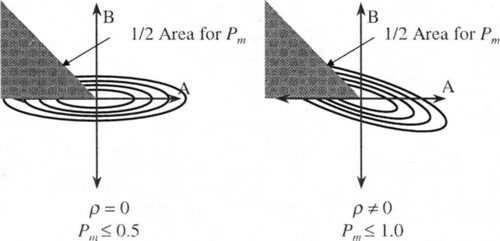
The ellipsoid represents a bivariate normal distribution, and the octant is the area where the effects of higher-order Walsh coefficients contradict and overrule those of lower order. The rotation of the ellipsoid in the plane is caused by ρ, and “length” of the ellipsoid is caused by the ratio of σa to σb, coupled with ρ. For ρ = 0, the major and minor axes of the ellipsoid align with the axes of the plane. Note that in this uncorrelated case, the maximum value of Pm is 0.5, since (for large σa / σb), at most 1/4 of the ellipsoid is in the octant. Previous investigations [10] empirically demonstrated that this was the case for NKP landscapes, and thus their juxtapositional complexity was limited. Note that in the correlated case, Pm can approach 1.0, since up to 1/2 of the ellipsoid can fall beneath the octant.
6 New Generation Methods
Figure 1 illustrates that to manipulate juxtapositional complexity, one must stretch and rotate the “tongue” of the ellipsoid into the fourth octant. This involves two factors: the relative scale of the sums of higher and lower (odd) ordered Walsh coefficients, and the correlation of these sums. This suggests a class of methods can be developed that use the Walsh generation procedure suggestion in Section 4, and direct manipulation of the relative scale of correlation of normally generated Walsh coefficients.
7 One Such Generator
There are quite a number of ways to develop generators based on these principles, given that there are several values of K for which one can consider the relative scales and correlations. Moreover, these scales and correlations are interrelated, given that they involve progressive sums of Walsh coefficients.
Also, note that there are a number of ways to correlate random variables, such that they yield the desired marginal distributions and correlation in the sample of landscapes [8]. Some methods are less appropriate to our goal of constructing a landscape generator than others. For instance, one could use a mixture of maximally correlated pairs and uncorrelated pairs.
With this structure, one number xA could be randomly generated from a standard normal distribution. Then, with a preselected probability p, another number xB could be taken as a linear function of xA, and with probability 1 − p, xB could be set as an independent random variable.
Such a procedure could give a generator that had the desired correlation characteristics over the space of xA, xB pairs. However, if these numbers were used in the generation of landscapes, it would not yield a situation where any one landscape had some desired complexity characteristic.
A more desirable procedure is to generate xA randomly from a standard normal distribution, and generate xB as follows:
![]()
where σ(0, 1) is another standard normal, and R is a parameter, − 1 ≤ R ≤ 1. This method produces the correlated standard normal random variables, and the correlation will have the same sign as R. However, note that the correlation will not necessarily have the same magnitude as R.
Using this correlation procedure, we have implemented the following generator:
Given an even value of K, set all Walsh coefficients to zero:
A Set i = 1, and identify all the Walsh coefficients wj (subpartition coefficients belonging to the first partition) of order K or less indicated in the (randomly generated) set of P partitions.
B Set a counter countj to equal the number of partitions within which each wj has an effect.
C To each wj add a random number xj, taken from a standard normal distribution with mean zero and variance  . If wj is of odd order, add xj to the running sum sumi, and xj2 to vari.
D Repeat for each partition i = 2,…, P.
E Set the P order K + 1 Walsh coefficients indicated by the set of P partitions, using the following formula:
![]()
where the sum is taken over odd ordered subpartitions, the S is a scale parameter, and R is a correlation parameter, which ranges from -1 to 1. One determines the fitness of an individual as in steps C through E in Section 4. Note that the complexity of step A is to limit unintentional cross-correlation between overlapping subpartitions.
Note that R controls correlation between higher and lower order coefficients, and small S yields higher order coefficients that are much larger than those of lower order, within the same partition. Thus, one would expect more juxtapositional complexity with lower S, and more highly negative R.
This landscape procedure involves 5 parameters: N, K, P, S, and R, and are thus referred to as NKPSR landscapes. Although the additional parameters may seem to complicate manipulating these landscapes, previous work [10] shows that one must be able to manipulate each of these aspects of a landscape to manipulate peak distribution and juxtapositional complexity.
In summary, the landscape has the following parameters:
(1) N - size of the landscape,
(2) K - the size of largest epistatic partitions,
(3) P - number of epistatic partitions,
(4) S - the relative scale of lower and higher order effects in the partitions,
(5) R - correlation between lower and higher order effects in the partitions.
8 Observations About the New Generator
Given our previous work, we wish to consider three aspects of the generator; peak distribution characteristics, juxtaposition characteristics, and, finally, performance on the landscapes using a real GA. Each of these is considered in the following sections.
8.1 Peak Distribution Characteristics
In order to evaluate the properties of NKPSR landscapes, a number of landscapes were created for each of a set of combinations of parameter values. For landscapes of size N = 12,14,16,18 and 20, 10 landscapes were created for each of the valid combinations of the following parameters:
P = {4, 8, 16, 32, 64}
R = (-0.81, -0.2, 0.0, 0.2, 0.81}
S = {0.01, 0.1, 1.0}
Each landscape was exhaustively probed in order to discover the location and value of all the optima (both local and global), and the following values were then calculated for each landscape:
• Maximum, minimum, mean and standard deviation of fitness,
• Mean and standard deviation of optima fitness,
• Number of optima, mean and standard deviation of distance of optima from the global optimum,
• Correlation between relative fitness of local optima and distance from the global optimum.
The results were subjected to a one-way analysis of variance (ANOVA) for the factors N, K, P, R and S, and to tests for linearity. The results are summarized in Table 2. Where the ANOVA tests indicate statistical significance at the 1% level, the ε2 value (a measure of the proportion of the variance in the measured value that can be attributed to the factor) is given where the factor accounts for more than 1% of the observed variance. Particularly meaningful values are shown in bold, and a hyphen indicates that the ε2 value is less than 5% although the ANOVA results show that the factor is significant. In all cases, NSS indicates no statistical significance. Where a factor appears to be a major determinant in the value of the variable, and tests suggest a significant linearity between the values of the factor and the observations, the correlation co-efficient is shown in braces.
Table 2
Statistical factors indicating the effects of N, K, Pand S on peak distribution characteristics of landscapes. The Optima Correlation row pertains to the correlation between local optima fitness, and distance from the global optimum.
| Measure | N | K | P | S |
| Landscape Max. Fitness | - | 0.4979 (0.6982) | 0.2909 (-0.4518) | - |
| LandscaPe Min. Fitness | - | 0.4972 (-0.6979) | 0.2926 (0.4528) | - |
| Land Std. Dev. Fitness | - | 0.4051 (0.6309) | 0.4669 (-0.5329) | - |
| Mean Fitness Local Optima | - | 0.4221 (0.6459) | 0.4281 (-0.5416) | - |
| Std Dev Opt. Fitness | NSS | 0.3807 (0.6086) | 0.1547 | 0.1180 |
| Number of Local Optima | 0.1821 (0.3671) | 0.05177 | 0.1087 | - |
| Mean Distance | NSS | 0.1210 (0.3156) | - | 0.1385 |
| Std. Dev. Distance | 0.4384 (-0.6567) | 0.1585 | - | 0.0913 |
| Optima Correlation | - | 0.3134 (0.5444) | 0.0606 | 0.1588 (-0.3945) |
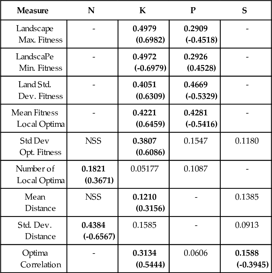
The analysis shows that the factor R is not statistically significant for the distance related measures, and never accounts for more than 2% of the observed variance in the fitness related measures, and so this column is omitted for clarity.
From these results we can observe that as with the NKP landscapes, the dominant factors affecting these coarse peak distribution statistics are N, K and P.
Previously reported analysis on NKP landscapes [10] showed that the major effect of P was as a kind of “gain control”, altering the spread of fitness values present in the landscape but not affecting the location of peaks. This is a secondary effect arising from the fact that if partitions overlap it is not possible to simultaneously optimise them all, and as the number of partitions increases so do the number of partitions with sub optimal values in optima. This effect can be seen again in these results, and there is an additional affect that P now accounts for over 10% in the observed variance in the number of peaks, the number reducing as P is increased.
Unlike the NKP landscapes, the value of K now has a significant effect on the range of fitness values present, with both the range of fitness value, and the mean fitness of local optima increasing with K. This can be explained by the fact that as K increases, so the number of low order Walsh coefficients within each partition increases, with a corresponding increase in the variance of the normal distribution from which the high order coefficient is drawn.
As K increases, the mean distance of local optima from the global optimum, the mean and standard deviation of their fitnesses (relative to that of the global optimum), and the positive correlation between fitness and distance from the global optimum all increase, reflecting the pattern observed by Kauffman of a “massif central” present at low K but disappearing as the K increases.
The significant (i.e. ε2 > 1%) effects of S as it increases from 0.01 to 1.0, (i.e the high order co-efficients become less important) are:
• the mean distance of local optima from the global decreases
• the correlation between their fitness and that distance becomes more negative
• the standard deviations of both fitness and distances increases.
The first two observations can be understood when it is considered that the scale factor S stochastically affects whether the high order co-efficient outweighs the effect of the low order values in determining the location of the global optimum: S approaches 1.0 there is less chance of creating a misleading landscape.
The effects of S on the peak distribution characteristics are more clear when a single set of values are considered for N,K and P, for example the correlation values for N = P = 16, K = 2 with R = − 0.81 are − 0.2278 for S = 0.01 and − 0.5520 for S = 1.0.
However when N,K,P and S are fixed, the effects of changing R are not statistically significant, suggesting that these peak distribution characteristics are perhaps too coarse to detect the effects of a single deceptive global optimum
In conclusion it would appear that in terms of the peak distribution metrics, the characteristics of the NKPRS landscapes are broadly similar to those of the NKP landscapes, and are largely determined by K, with secondary effects due to S as noted. These metrics are based on measuring distance in Hamming space, which more closely reflects search conducted by “bit-flipping” hill climbers and mutational operators.
8.2 Juxtapositional Characteristics
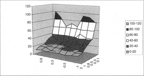
To evaluate the effects of the various parameters of NKPSR landscapes on juxtapositional complexity, 40 landscapes were generated for a number of combinations of these parameters, and the results were used to calculate the probability of misleadingness, as discussed in Section 5. Typical results of this exploration are shown in Figure 2 through Figure 5.
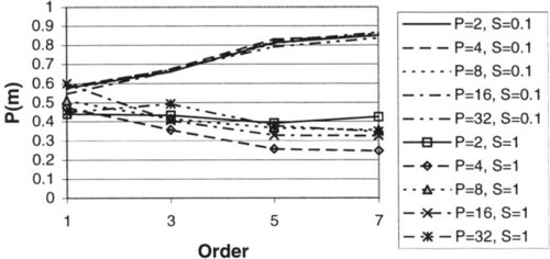
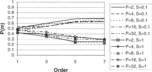
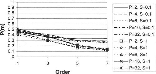
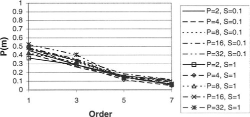
Note that, as one would expect, the complexity of the landscape increases with negative R. P also has a noticeable effect. Complexity also increases with decreasing S, as one would expect.
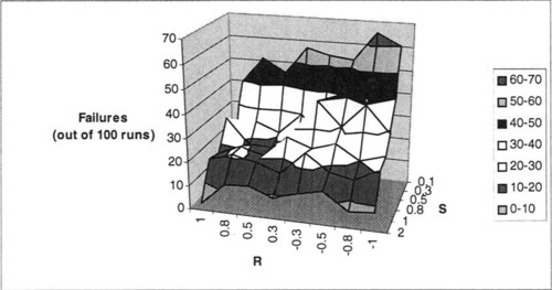
8.3 GA Performance
The previous sections show that over the space of possible landscapes of a given size N, one would expect K and S to have the most effect of peak distribution, while K, S, and R should have effects on juxtapositional complexity. Whether these effects result in actual complexity for the GA remains to be established. To examine this issue, we applied a relatively simple GA to a selection of problems constructed with this generator.
The GA used a population of 100 binary individuals, with uniform crossover, applied with probability one, point mutation applied with probability 0.05, and tournament selection. This GA was in no way optimised for these problems, since we simply wished to illustrate variations in GA performance over the space of landscapes generated. For each set of generator settings, the GA was run 100 times: 10 random restarts on 10 separate landscapes.
In each landscape, we exhaustively located the optimum, and ran the GA until it either found this point, or completed 300 generations. We recorded the number of GA runs that located the optimum, and the number of generations to find the optimum in those cases.
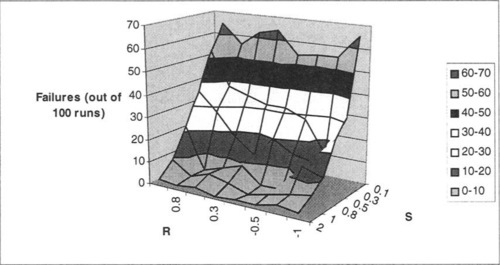
Figure 6 shows the results of the GA for N = 15, K = 2, and P = 15. Note that this yields 3-bit interactions, and the number of partitions typical in NK landscapes. As expected, this figure shows increasing difficulty for the GA as S becomes smaller and R becomes more negative. However, note that for large values of S (where problems are relatively easy for the GA), distinctions in R become less important.
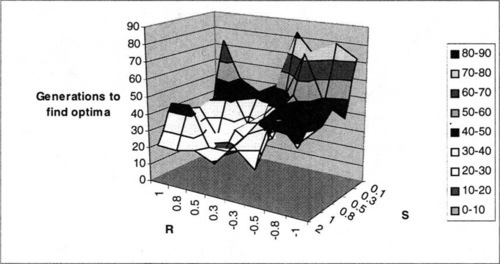
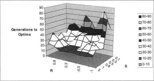
Similar results are seen by observing the number of generations needed to locate the optimum, for the runs where the optimum is found (see Figure 7).
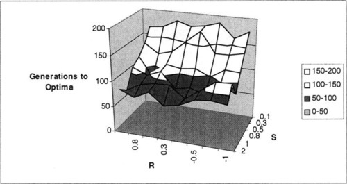
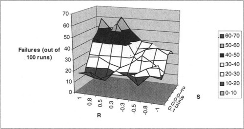
However, it is interesting to note that the pattern shifts for higher levels of epistasis. Consider the results for K = 4 and P = 15, shown in Figure 8 and Figure 9. Note that in Figure 8 the S axis is shown in reverse order (relative to previous plots) for clarity. As one would expect, these problems, which have higher order Walsh coefficients, become more difficult for the GA to solve. However, at this level of epistasis, it seems that the effect of S (scale) is reversed. High S yields problems that are more difficult for the GA, in terms of actually finding the optimum. This runs counter to the intuition of our previous analysis. However, note that Figure 9 generally shows the familiar pattern predicted by our analysis. Apparently, the effects of Walsh coefficient scale change, in some way that is unexplained by our current analysis. For such landscapes, the optimum becomes more difficult for the GA to discover with higher S. The effects of R are less clear, although the seem to follow the pattern predicted by analysis for intermediate values of R, shown in Figure 8. However, when the optimum is found by the GA, the number of generations increases with lower S, as our analysis would suggest.

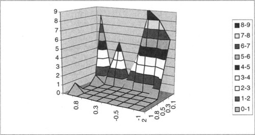
It is also interesting to examine patterns of performance with respect to S and R for low values of P. These problems are generally easy for the GA. For instance, consider results for K = 4 and P = 5 shown in Figure 10 and Figure 11. There is still some pattern of declining difficulty with increasing S and more negative R, particularly in the generations-to-optimum results, shown in Figure 11.
It is also useful to observe landscape behaviour for levels of P greater than N. Figure 12 and Figure 13 show results for K = 2 and P = 20. In this case, the pattern of increasing difficulty with decreasing S is shown in both success in finding the optimum, and the number of generations required. A general pattern of increasing numbers of generations to find the optimum with more negative R is generally observed as well (Figure 13). However, the effects of R on success of the GA in finding the optima (Figure 12) are less clear, and seem to sometimes reflect the opposite of the expected, giving decreasing difficulty with lower and more negative R, particularly for the intermediate values of S.
Finally, we consider results for K = 4 and P = 20, shown in Figure 14 and Figure 15. As in previous plots with K = 4, note that Figure 14, has the S axis reversed, since the effects of S on the GAs ability to find the optimum are generally the opposite of our intuition. Moreover, in this case (and in other higher K and P scenarios), the effects of R seem reversed, as well. However, in the generations-to-optima results (Figure 15), the results stay relatively consistent with our analytical intuitions, as they have in our other experiments.

9 Final Comments
We believe that the addition of a correlation (R) and scale (S) parameter to the landscape size (N), epistatic partition size (K), and number of partitions (P) parameters, yields more adequate controls over the complexity in randomly generated landscapes.
The results presented from a series of runs with a “vanilla” GA show patterns which indicate that an important factor is the degree of overlap between partitions, which governed by the combination of K and P. For low overlap, the behaviour is much as predicted, with the values of S and R providing a useful extra method for controlling “GA difficulty”. As the amount of ovelap between partitions increases however, the behaviour of the GA changes (with respect to S) so that although the time taken to locate the optimum still behaves as predicted, the frequency with which the optimum is found decreases as S approaches 1.0. A likely explanation is that the increased overlap is introducing spurious low order effects, which are outweighing the effects of the high order co-efficients unless the scale factor is high enough. Development of new generators which attempt to avoid this problem remains a topic for future research.
We believe random landscapes with appropriate controls will allow for more general exploration of performance and robustness of a variety of GA configurations, and of other search algorithms. The exploration may also yield deeper insights into the general nature of search landscape complexity itself.