20
Introduction to the Mathematics of Financial Markets
20.1 Introduction
This chapter will introduce some basic concepts of modern mathematical finance. One goal is to cover the fundamentals of option pricing. This has become an important tool in actuarial mathematics, since many insurance and annuity contracts today contain the so-called ‘embedded options’, which we discussed in Section 13.2. For the most part, we carry this out in a discrete setting, but we do move into the continuous-time approach briefly in order to introduce the Black–Scholes–Merton formula. Another major objective in this chapter is to revisit the basic quantity of a discount function which we introduced early on. In the first part of the book, we treated this as a deterministic function, but a more realistic approach would be to consider v(s, t) as a random variable, reflecting the stochastic nature of investment returns that we discussed in Chapter 14. In particular, we seek a version of the key identity, Formula (2.1) in this stochastic setting.
A prerequisite for this chapter is the starred Section 2.12. We assume familiarity with concepts discussed in that section such as as short selling, forward contracts, and arbitrage.
20.2 Modelling prices in financial markets
A financial market is an institution designed to facilitate the trading of financial assets, such as stocks or bonds. Certain individuals wish to buy such assets, while others wish to sell them, and the financial market provides a forum to bring together the various parties. The potential holder of an asset quotes a desired selling price, known as the asking price, while the potential buyer quotes a desired buying price, known as the bidding price. When bidding and asking prices are equal it establishes a price for the asset, and a sale can be made. Our goal in this section is to develop a stochastic model for the evolution of prices.
For most of this chapter, we assume a relatively simple framework, which will allow us to present the main ideas without too many technical mathematical difficulties. We assume a discrete-time model. That is, trading of assets will take place at integer times 0, 1, 2, …. The time period can be arbitrary, and we can think of it as possibly a very short time, (say an hour or even a minute) which could then constitute an approximation to the more realistic continuous-time setting. We adopt a finite-time horizon, with time N as the last date we are interested in. Finally, we assume that the price of any asset can take on only finitely many possible values.
Suppose we have M + 1 assets traded in our market, numbered from 0 to M. We will let
We consider each such price as a random variable. Therefore, our financial market is modelled by M + 1 discrete time stochastic processes Sj(n), where j = 0, 1, 2, …M, and n = 0, 1, …N.
We will single out a particular asset, often referred to as a bank account, for asset numbered 0. To describe this, we will first need to postulate in our model a nonnegative quantity r called the risk-free rate of interest, which is the interest rate that we can obtain on a risk-free investment as described in Section 2.12.
We can then define this asset by
In other words, this is an asset which accumulates at the risk-free interest rate. It is a stochastic process in which each random variable takes a single value with probability 1. For simplicity, we are at first adopting a constant risk-free interest rate. The definition could be based on a more general discount function and we comment on this below in Section 20.13.
We will make the same idealized assumptions that we made in Section 2.12. That is, we postulate that for each asset, any real number of the units can be bought at any trading date. Through short selling if necessary, this includes negative quantities. We also assume that there are no transaction costs such as commissions.
Note that the existence of the bank account means that we are assuming that all participants in our market can freely borrow at the risk-free rate.
Another simplifying assumption made throughout is that none of our assets provide any payments at intermediate dates, such as dividends on stocks or coupons on bonds. They provide funds only upon sale or maturity.
20.3 Arbitrage
An initial observation is that in the typical financial market, the various asset prices do not move independently. If asset i moves up in price, asset j may have a tendency to move up, or possibly to move down, or be certain to move up or down. It can be quite complicated to model all dependencies, but the no-arbitrage principle will often enable us to reduce the possibilities. In our stochastic models, this requires a more complicated definition than the one we gave in Section 2.12.
We first define the concept of a trading strategy. This is roughly a description you, as an investor in the market, would give to an assistant before leaving for a holiday on a remote desert island where you cannot be reached. You would specify the number of units of each asset to be held at each time period. At each trading date after the initial portfolio is established at time 0, certain assets in the existing portfolio would be sold and others bought to achieve the stipulated amounts. These amounts could depend on the entire past and present history. The description could be enormously complicated or quite simple. For example, a trading strategy might be as follows:
Start with an initial portfolio of 1 unit each of asset 1 and asset 2. Keep this intact until the first time that the price of asset 1 is above 40 per unit and the price of asset 2 is below 30 per unit. At that time, sell all units of asset 1 and use the proceeds to buy shares of asset 2. These are then held without further trading.
Note that the amounts to be held at time n can depend on all the prices of all assets at or before time n, but not after. It would not be a feasible trading strategy to specify that a a certain asset should be sold at time 2, if the price of some other asset were below 40 at time 3.
To formalize this somewhat, we can represent the asset holdings at any time n by a vector
where αj(n) is the number of units of asset j held at time n.
The entries of this vector are random, depending on the prices up to time n. So a trading strategy ![]() is formally a vector of these random vectors.
is formally a vector of these random vectors.
where each α(r) is a function of the values of Sj(k) for j = 0, 1, …M, k = 0, 1, 2…r.
For any trading strategy and any time n, we will have a portfolio consisting of a certain number of units of each of our M + 1 assets. The portfolio at time n will then then have a value V(n) obtained by multiplying the number of units of each asset by the price of that asset at time n, and summing. That is
a random variable depending on all prices as well as the trading strategy as followed up to time n. Of course V(0) is a definite number as it is the cost of setting up the initial portfolio at time 0 when all prices are known.
For any trading strategy, there is a reverse strategy which involves holding at each time, the negative of the number of units held in the original strategy. In other words, one sells in place of buying and buys in place of selling. Formally, if a trading strategy is given by the the vector ![]() , the reverse strategy is given by
, the reverse strategy is given by ![]() . If V* denotes values for the reverse strategy it is clear that V*(n) = −V(n) for all n.
. If V* denotes values for the reverse strategy it is clear that V*(n) = −V(n) for all n.
Here is another important concept.
Definition 20.1 A trading strategy is said to be self-financing if for any trading date after time 0 and before time N, the total price of all the assets sold on a given trading date exactly equals the total price of all the assets bought on that date, so no additional infusion or withdrawal of capital is required.
For a self-financing strategy, the value of the portfolio at any intermediate trading date is the same before and after trading.
We can now summarize the procedure we will be following in subsequent discussions. We set up an initial portfolio at time 0 for a cost of V(0), dictate a self-financing trading strategy, retreat to the dessert island, where no additional outlays of cash are required and none are received. Finally, the portfolio is liquidated at time N for proceeds of V(N), a random variable which depends on both the trading strategy and the evolution of prices. We let P denote the probability measure for V(N).
The key definition of this section can now be given in terms of the starting value V(0) and the ending value V(N).
Definition 20.2 The financial market admits arbitrage if there exists a self-financing trading strategy such that
A financial market which does not admit arbitrage is said to be arbitrage-free.
In other words, an arbitrage opportunity is one where starting with a zero investment, we cannot possibly lose by the end of the trading period, and we have at least some chance of making a gain. Note that the arbitrage opportunity does not guarantee a positive gain. One can think of it as being given a lottery ticket for free. We cannot lose anything, and there is some chance of profiting. It is important to note that cases where there is a very small probability of loss do not constitute an arbitrage under this definition. The avoidance of the loss must be absolutely certain.
Remark In the definition of arbitrage, we could replace the condition on V(N) by V(N) ⩽ 0 and P[V(N) < 0] > 0, since, if this holds, the reverse strategy will satisfy the original condition. This looks a bit strange at first, but it simply says that if there is a strategy for which we are sure not to gain, then the reverse strategy is sure not to lose.
An important consequence of the above is the following.
Theorem 20.1 In an arbitrage-free financial market, if there is a self-financing trading strategy for which V(n) is a constant c for some n, then
Proof. Modify the strategy by holding − V(0) units of the bank account at time 0, so that the new strategy has initial value 0. If necessary, modify the strategy further to stipulate that everything should be settled at time n, and the proceeds (possibly negative) left to accumulate in the bank account at the risk-free rate until time N. The new strategy will have the constant value of c − V(0)(1 + r)n at time n, and this must be equal to 0. If not, there would be a sure chance of having either a positive or negative amount at time N, which would imply an arbitrage opportunity, by Definition 20.2 and the remark following this definition.
![]()
This was a reasonably simple result, but there is an important message behind it. It says that in the absence of arbitrage, if we can find a self-financing trading strategy which eliminates risk at some point, then our initial investment must accumulate at the risk-free rate up to that point.
Remark It is true that any trading strategy can be converted into a self-financing one by using the bank account. An excess of the sales over purchases can be placed in the bank account, while excesses of purchases over sales can be handled by borrowing. However this gives a different strategy with a different amount held in the bank account at time N, and therefore a different value of V(N). The self-financing hypothesis is therefore essential in the definition of arbitrage.
For our first example, we consider a very simple financial market. We will take N = 1, so a trading strategy involves simply specifying the initial portfolio. Our financial market has, in addition to S0, a single risky asset S1 consisting of a stock. We can assume, changing units if necessary, that the price of a unit of the stock is 1 at time 0. Suppose that the price of the stock at time 1 can only take two possible values, u or d (standing for ‘up’, ‘down’ respectively) with d < u, each with positive probability. We call this a binomial model to reflect the two possible values at time 1.
Theorem 20.2 The above financial market is arbitrage free if and only if
Proof. Consider any trading strategy with V(0) = 0. If α is the number of units of stock in the initial portfolio. we must have − α units of the bank account. Then we will have either V(1) = αu − α(1 + r) or V(1) = αd − α(1 + r). Suppose (20.1) holds. If α < 0 then the first such value will be negative and the second will be positive, while the reverse holds if α > 0. If α = 0, both values are 0. An arbitrage opportunity cannot exist.
Conversely if (20.1) is not true, then at least one of two possibilities holds. Suppose d ⩾ (1 + r). We create an arbitrage opportunity by choosing α > 0 which makes both values of V(1) nonnegative,with at least one positive. The other possibility is that u ⩽ (1 + r), in which case we similarly create an arbitrage opportunity by taking α < 0.
![]()
Note that the converse statement is intuitively obvious. If the inequality does not hold, then we can create an arbitrage opportunity by either buying a stock which is sure to yield more than the risk-free return, or short selling a stock which is sure to yield less than the risk-free return.
Another pertinent fact to notice in the definition of arbitrage is that the condition does not depend on the particular values of P but only on whether such values are positive or zero. We are therefore led to make use of the following standard definition of probability theory.
Definition 20.3 Two probability measures P and Q on a sample space S are said to be equivalent if for all A⊆S, we have P(A) = 0 if and only if Q(A) = 0. (For readers familiar with the concept of an equivalence relation, one can readily verify that this is a legitimate such relation.)
It is clear from the definition that a financial market is arbitrage-free with respect to P if and only if it is arbitrage-free with respect to any equivalent probability measure Q.
20.4 Option contracts
Given a financial market, we can do more than just buy or sell the existing assets. We have already seen one possibility, which is to enter into forward contracts. Another possibility is option contracts. These are in one sense similar to forward contracts since they are both transactions which involve trading of assets at a future date for prices that are specified now. There are major differences however, for in an option, unlike the forward contract, one party is not obligated to complete the transaction, but has the option to do so, and will only exercise this option if it is advantageous. There are two basic types of option contracts, known as calls and puts. A buyer of a call option has the right to buy a specified asset at a specified future time, known as the expiration date or exercise date, for a specified price, known as the strike price or exercise price, if they should choose to do so. The call option buyer has a similar motivation to a speculator taking a long position in a forward contract. They hope for a rise in price, so that they can buy the asset at a price which is lower than prevailing at the time of purchase. If the price of the asset at the expiration date is below the strike price, the option will not be exercised. A buyer of a put option has the right to sell a specified asset on the expiration date for a specified strike price. The put option buyer has a similar motivation to the speculator taking a short position in a forward contract. They hope for a fall in price so that they can sell the asset for more than it is worth at the time of sale. In this case, if the price of the asset at the expiration date is above the strike price, the option will not be exercised. Unlike the forward contract, the call and put buyers are not on opposite sides. For each of them, there must be another party who sells or (as it is commonly said) writes the option, and agrees to complete the transaction should the option holder so elect. Now if the option is exercised, the option writer is necessarily selling or buying at an unfavourable price, and they are compensated for this by the option price which they receive from the option holder at the time the agreement is entered into. The option writers of course hope that options will not be exercised, so they profit by the full amount of the option price, and do not have to engage in an unfavourable transaction. Determining option prices is complicated, and will form much of the material of this chapter.
It should be noted that what we have described are more properly known as European options, which specify that the option can only be exercised on the one specific expiration date. We will assume all options we discuss are of this nature unless specified otherwise. Another type of contract, known as an American option, allows for the exercise of the option at any time before or on the expiration date. These are more complicated and will be dealt with briefly in Section 20.7.
Although the underlying assets for calls and put are normally taken as financial instruments like stocks, as will be the case in our treatment, the basic idea of an option arises in many diverse contexts. For example, buying insurance on an asset like a house, is essentially buying a type of put option. You are protecting yourself from a drop in value, not from market variation in this case, but rather from physical damage. Similarly, the guarantees for variables annuities (as discussed in Section 13.2) which protect your account against unfavourable investment experience constitute put options. For another example, suppose that you take out a long-term loan or mortgage, and the lender gives you the right to repay in full at any time without penalty. In effect, you have been given a call option. In this case, you are protected from a rise in the cost of repayment, which will occur if interest rates decline. (Refer to the discussion in Section 2.10.3.)
In essence, protection against declines in the value of an asset that you own, while allowing you the full benefit of increases in value, can be viewed as being given a put option. Protection against increases in the value of an asset that you may wish to acquire in the future, while allowing you the full benefit of decreases in value, can be viewed as being given a call option. Note that in contrast, forward contracts protect you from unfavourable declines or increases, but they do not allow the parties to reap the full upside benefits, since the transactions must be completed with the agreed upon prices.
20.5 Option prices in the one-period binomial model
In this section, we show how the no-arbitrage principle allows us to calculate an option price for the one-period binomial market where condition (20.1) holds. We illustrate with a particular example. Suppose that a share of the stock is selling for 108 at time 0 and at time 1 it will be either 132 or 99, each with positive probability. Assume a risk-free interest rate of 10%.
Consider a call option on the stock with an expiration date of time 1 and a strike price of 110. What should the price per unit of this option be? At first, one may think that there is no way to determine this exactly, and that it could take on many possible values. After all, the option is just another asset with its price being determined by the amounts bid and asked by the various market participants. The worth of this asset, however, is directly tied to the performance of the stock, so it should be clear that its price must be related in some way to the stock price. Such an asset is often termed a derivative security, since its value is derived from that of another security.
To help determine the price, we take the following point of view. Purchasers of call options are not normally interested in actually taking possession of the stock at maturity. They simply want to buy it at the strike price, and sell it immediately for the higher market price if available. If the market price is below the strike price, the option is worthless and they receive nothing. The option then is just another asset S2 with S2(1) = 132 − 110 = 22 if the stock price goes up, or S2(1) = 0 if the stock price goes down. The problem is to determine S2(0).
Those well-versed in the actuarial models we discussed in earlier chapters may well think that we can determine S2(0) by simply taking a discounted expected value, as we did with several other similar sounding problems. That is, we simply take the price as 22vp where v is the discount factor for one period, and p is the probability that the stock goes up. We will first illustrate why one cannot solve the problem this way, and after that, we will, paradoxically, illustrate why one can do it this way.
The first problem is that one is not given p as part of the model. All that we postulated about the probability measure P was that both of the possible outcomes at time 1 have positive probability. Indeed, there may not be any reasonable choice for a single value of p. The many different participants in the market may well have completely different assessments of this figure. It is not unusual to find two experts commenting on a particular stock, where one claims it is the best buying opportunity to come along in the last decade, and the other predicts imminent bankruptcy of the firm.
The second problem is that one is not given v. Now the reader may take issue with this statement since we postulated a risk free rate of 10% a few paragraphs back, so it appears as if v is simply (1.10)− 1. Use of this rate would imply that the buyer is looking for an expected return of 10% on their investment. However, 10% is the return for a perfectly risk-free investment. Investing in a call option is far from being risk-free. If the stock price at expiry is below the strike price, the entire investment is lost. It is to be expected that a rational option purchaser will want a return in excess of 10% as compensation for taking on the risk. (Recall that we discussed the same concept when introducing the risk discount rate in Section 12.4).
We will now solve the puzzle, and show that regardless of the assessment of p or of the desired yields of different individuals, the price of this option can only be 12. The reason is that one can in fact replicate the option for an initial investment of 12. That is, by investing only in the bank account and the stock, one can produce an outcome at the expiration date, which matches exactly the payouts of the option. This is done by buying 2/3 of a share of stock at time 0, which will cost 72. We can put in 12 cash, and borrow the additional 60. If the stock price is 132 per share at time 1, we sell our 2/3 of a share for 88, pay off the loan balance which is now 66, leaving us with 22. If the stock price is 99, we sell our 2/3 of a share for 66, and pay off the loan, leaving us with nothing extra. We have therefore exactly replicated the option for the price of 12. It is is clear that no one would pay more than 12 to buy this option. Similarly, nobody would sell the option for a price of less than 12, since instead they could reverse the above strategy and be in the same position at time 1 as if they had written the option, but they would have have received 12 at time 0.
Here is another point of view, which ties in with our previous definition of arbitrage. If we enlarge our financial market by adding the option as another asset S2, then we must take S2 = 12 to make this enlarged market arbitrage-free. To take a definite example, suppose the option price is 13. We will construct an arbitrage opportunity. Take the trading strategy which has as initial portfolio α(0) = ( − 59, 2/3, −1). The reader can verify that V(0) = 0. Now S0(1) = −64.90, so If S1(1) = 132, then S2(1) = 22 and V(1) = 1.1. If S1(1) = 99 then S2(1) = 0 and again V(1) = 1.1. We leave it to the reader to find an arbitrage opportunity if the option price is below 12.
Let us now go back to the proposed solution of of 22vp as an option price, which we criticized a few paragraphs above. If we in fact use the risk-free rate and therefore take v = 1.10− 1, we will get the correct answer by using p = 0.6. Is there someway we could have discovered this probability of 0.6 beforehand? The answer is yes. Let us suppose that there exists a so called risk-neutral individual, that is one who ignores the risk and is happy to accept an expected 10% return on any investment, regardless of the degree of safety involved. Let p be the particular probability of rise in the stock price, which would be assumed by such a risk-neutral person. In order that this person would be willing to pay 108 for a share of stock, we should have that
and solving we have indeed that p = 0.6.
We have now discovered the important principle of risk-neutral valuation. The assignment here of 0.6 and 0.4 to the events of the stock going up or down, respectively, is known as a risk-neutral probability measure. It is the probability that must be assigned by a risk-neutral individual in order to justify buying the stock at the market price. Note that we are not saying that such a person necessarily exists, and indeed have stressed that most investors would be unlikely to possess such an attitude. We are only saying that if one did exist, the price of the underlying asset would necessarily imply a unique probability assessment for that individual. The principle then says that if we use the risk-free interest rate, along with the risk-neutral probability measure, then we can indeed value options by following the usual actuarial approach of taking a discounted expected value.
Note carefully that the risk-neutral probability measure need not be the same or indeed have any particular relation to the original measure P, other than being equivalent in the sense defined above. Even if we had specified values for P, these would have had no effect on the resulting option price. The fact that one can risklessly replicate the option means that only the risk-neutral probability and the risk-free interest rate need be considered.
This is a puzzling observation at first, and for those who are still skeptical, we will look into the situation a little further. We mentioned above that the probability p was not even specified as part of the model, but let us suppose it is. In fact, suppose that instead of a stock with uncertain returns, we have two lotteries each depending on the same random draw. A ball is drawn randomly from an urn containing two white balls and one red. The payoff from lottery 1 at time 1 is 132 if a white ball is drawn, or 99 if a red is picked. The payoff from lottery 2 at time 1 is 22 if a white ball is drawn or 0 if a red is drawn. So the true underlying value of p is now indisputable as 2/3. If the price for a lottery 1 ticket is 108, and we make the assumption that we can buy or sell any fraction of lottery 1 tickets, then the price for a lottery 2 ticket must be 12, by exactly the same argument as given above, regardless of the known value of p. What does this imply for people who participate? Buyers of a ticket in lottery 1 are in effect earning an expected return of [(2/3)132 + (1/3)99)]/108 − 1 = 12.04%. There is a reasonable extra return over the risk-free rate, to compensate for the risk taken on. Buyers of a ticket in lottery 2 are in effect earning an expected return of [(2/3)22/12] − 1 = 22.22%, a much higher return, which compensates for the greater risk in lottery 2 when the entire stake could be lost. Indeed for any value of p above 0.6, there will be a return above the risk-free rate in lottery 1 and an even higher return in lottery 2. It is only for the risk-neutral value of p equal to 0.6, for which the expected returns on both lotteries will coincide with the risk-free rate.
Going back to our original example with the stock, is it possible that an investor who assesses the probability of an upward movement as being less than 0.6 would still pay 108 per share, thereby earning an expected return of less than the risk-free rate? This may seem irrational, but it is no more so than the behaviour of a vast number of people who buy lottery tickets or gamble in casinos at highly unfavourable odds. (For more on this topic, see Example 22.2.)
We next derive a general formula. Suppose that (20.1) holds. As we did above, we can set up an equation to solve for p, the risk-neutral probability that the upward move will occur. Taking S1(0) = 1, this is
which we solve to obtain
Note that condition (20.1) ensures that 0 < p < 1.
The above procedure allows us to uniquely price, not only call options, but a general derivative security in this market, which pays an amount A if an upward move occurs or B if a downward move occurs. We do this in one of two ways: first, we can find a replicating initial portfolio consisting of α units of the stock and β units of the bank account by solving the equations
Then
which is the cost of establishing the replicating portfolio. Secondly, and usually easier, we can bypass finding the replicating portfolio and just take the price as the discounted expected value of the the payoff with respect to the risk-free interest rate and risk-neutral measure. That is,
where p is as given in formula (20.20). The reader can verify that both methods lead to the same answer.
Example 20.1 For the example given at the beginning of this section, find the price of a put option with a strike price of 110.
Solution. If the upward move occurs, the holder tears up the option. If the downward move occurs, the holder buys the stock for 99, and sells it for 110. So this is a derivative security with A = 0, B = 11. Directly from Equation (20.20), we have that the price is 1.10− 1(0.4 × 11) = 4. Alternatively, solve (20.4) to derive the replicating portfolio given by α = −1/3, β = 40, and use (20.5) to get the same answer. To see this directly, we replicate the option for a cost of 4 by selling 1/3 of a share short, receiving 36, letting the total of 40 accumulate to 44 at time 1. This allows one to just cover the short position if the stock is up, or cover the short position and have 11 left over if the stock is down.
There is in this case yet another way to obtain the answer. In fact, we develop a general formula relating puts and calls.
Theorem 20.3 (Put-call Parity) Let γ denote the cost of a call option and π denote the cost of a put option on the same stock with a current price of S(0), the same strike price of K,and same expiration date N. Then
Proof. Suppose an investor at time 0 adopts the following trading strategy. Buy one unit of stock, sell one call option, buy one put option, and hold these without further trading up to the expiration date N. If S(N) > K, the put will expire worthless, the call will be exercised by the other party, so that the investor must give up the stock for a price of K. If S(N) < K, the call will expire worthless, the investor will exercise the put and sell the stock for a price of K, while if S(N) = K, both options are worthless and the value is just the stock price. Whatever happens, the value at time N of the portfolio will be K. Since V(0) is just the left side of Equation (20.20), the formula follows from Theorem 20.1.
![]()
The proof shows in fact that this theorem is true for a general arbitrage-free market, and does not depend on the binomial assumption. In our present example, we know γ = 12, N = 1, S(0) = 108 and K = 110, and we can immediately calculate that π = 4.
20.6 The multi-period binomial model
The model of the last section is clearly too simple to be representative of reality. As a further extension, we keep the binomial feature, but allow the prices to evolve over several periods.
We assume that the price of the stock evolves each period as described in the one-period model above. That is, if the value is s at the beginning of a period, the price at the end will be either su or sd where d < u. So for an initial price of S(0) at time 0, the price at time 1 will be either S(0)u or S(0)d, and the price at time 2 will be either S(0)u2, S(0)ud, or S(0)d2, etc. We can represent this by what is known as a binomial tree. See, for example, Figure 18.1 which is an example with u = 1.2, d = 0.8.
We can now consider any general contingent claim, which will be a payoff at time N which can depend on the entire history of up and down movements in the stock price. To formalize this, consider the sample space Ω consisting of all paths in the binomial tree. Each such path can be labeled by an N-termed sequence formed of the entries U and D, where U denotes an upwards branch and D a downwards branch, so there are 2N paths altogether. We postulate that there is a probability measure P on Ω, but we need not specify anything about it except that P(ω) > 0 for all ω ∈ Ω.
We now formally define the general type of derivative security we are interested in.
Definition 20.4 A contingent claim is a contract which provides a payment at time N which is dependent on the particular outcome in our underlying sample space. It is modelled by a random variable X, where for ω ∈ Ω, X(ω) is the payment for outcome ω.
For example, a call option with strike price K and expiration date N on a stock with current price S(0) is a contingent claim given by
whenever ω is a sequence with m upward movements and N − m downward movements. (For any real number t, the symbol t+ denotes max{t, 0}.)
A contingent claim can be more complicated than the options we have described up to now. Consider, for example, a lookback option on a stock which will return at expiry the maximum value of the stock over the period from time 0 to time N. So looking for example at Figure 18.1, we would have
and so on.
The multi-period model has the same essential features that we observed in the one-period model.
- The financial market consisting of the stock and the bank account is arbitrage-free if and only if condition (20.1) holds.
- Any contingent claim can be priced uniquely so as to prevent arbitrage. One method is to find a replicating self-financing trading strategy. The price of the claim is then the cost of setting up the initial portfolio for this strategy. A second way is to take the expected discounted value with respect to the risk-neutral probability measure Q on Ω, which is simply the measure obtained by applying the appropriate probabilities p or 1 − p as given by formula (20.3) to each branch of the binomial tree. That is, if ω has m entries of U and N − m entries of D,
These facts can be verified by using the results from the one-period model, and working backwards in time. The definition of contingent claim gives us directly its value at time N. We use those to determine the value and strategy applicable to each node at time N − 1, and then use these to get determine the value and strategy applicable to each node at time N − 2, and continue to iterate the procedure until we get to time 0.
Example 20.2 Consider a two-period model where the price of a stock evolves as shown by the tree in Figure 18.1 up to time 2, and r = 0.10. The contingent claim X is a call option at time 2, with a strike price of 92. So
Find the replicating strategy and the price of the option which will prevent arbitrage,
Solution. Suppose at time 1, the value of the stock is 120. We know that u = 1.2, d = 0.8, and we can solve the system (20.4) with A = 52, B = 4 to get α = 1, β = −920/11. This means that if the process is in the upper node at time 1, then in order to replicate the payoff at time 2, we should own 1 unit of stock, and carry a debt of 920/11. The total value V(1) is 400/11.
Similarly, if the value of stock is 80 at time 1, we solve the system (20.4) with A = 4, B = 0, and we arrive at a required portfolio of 1/8 units of stock and a debt of 80/11 for a total value V(1) of 30/11.
We now move back to time 0 and again solve the system (20.4) with A = 400/11 and B = 30/11, to obtain a initial portfolio consisting of 37/44 shares of stock and a debt of 7100/121. The value of this initial portfolio is V(0) = 3075/121 which must be the price of the option.
To summarize, one can replicate this contingent claim by the following self-financing trading strategy. At time 0, buy 37/44 units of the stock, using 3075/121 of one’s own capital and borrowing the remaining 7100/121 at the risk-free rate. At time 1, if the stock moves up, increase the stock holding to 1 unit, borrowing additional funds to do so. If the stock goes down, sell enough to reduce the stock holding to 1/8 unit, using the proceeds to partially repay the loan.
This replicating strategy gives in addition a hedging strategy. Suppose you have just sold such an option. You run the risk that the stock will move up both periods. If you do not actually own the stock, you will be required to buy it at 144 and sell it at 92 (which shows the danger of selling a so-called naked option on a stock you do not own). If you follow the trading procedure outlined above, you will be sure to be able to meet your obligation in any event, assuming of course that the given model for the evolution of the stock price is correct.
To calculate only the option price, rather than the complete replicating strategy, the second method can be used. That is
For the particular case of a call option with strike K, this takes the form
where p is determined by formula (20.20). In our case p = 3/4, and we can verify that, as before, the price is
Example 20.3 In the example given above, suppose the interest rate is 0. Find a price and self-financing trading strategy for the so-called lookback option, which pays at time N the maximum value of the stock at time 0, 1, 2.
Solution. The payoff is 144 for the outcome UU, 120 for the outcome UD, and 100 for each of the outcomes DU and DD. We can find the price exactly as we did for the option above. For r = 0 we can calculate p = 1/2 and
To find the trading strategy, we need a more complicated diagram. See Figure 20.1. In the original diagram (Figure 18.1), the paths of UD and DU both led to the same position at time 2. This is fine in cases where the prices of the stock at that point was all we were interested in, since this took the same value of 96 on both paths. However, in this case, the contingent claim is path-dependent and we need two different nodes to distinguish the two paths.
For the upper node at time 1, we need to hold α units of stock and β units of bank account where
so that
For the lower node at time 1 we similarly solve
so that
We are then back to a one period model with an asset that has value 132 if the upward movement occurs, or 100 if the downward movement occurs. So the initial portfolio must have α units of stock and β units of the bank account where
so that
So the trading strategy is to start with 116 (as we knew from the first solution above), buy 0.8 units of stock and put the rest in the bank account. If the upward move occurs, sell 0.3 units of stock, or if the downward move occurs, sell all 0.8 units of stock, in each case putting the proceeds into the bank account.
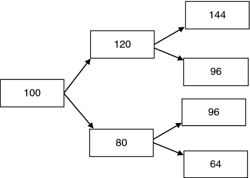
Figure 20.1 Example 20.3
For contingent claims which depend only on final prices, the first type of diagram, (like Figure 18.1) known as a recombining tree, provides a significant reduction in computation. This was not readily apparent in our simple example where N = 2, but suppose instead that N = 10. The recombining tree would have 11 final nodes, while the more general version would have 210 = 1024 final nodes.
20.7 American options
We include a brief discussion here on American options, which can have some surprising and initially puzzling features. Recall that such an option can be exercised at any trading date up to and including the final expiration date. One’s intuition tells us that the price of this should be greater than the price of the corresponding European option, since there is more choice and therefore a chance for more potential gain. However one’s intuition is not completely correct. In fact, given our assumptions, an American call option should never be exercised prior to the expiration date, so in fact the two options are equivalent and should bear the same price. If r = 0, the same phenomenon holds for an American put option. It is never correct to exercise early. However, in the more usual case when r > 0, it may well be correct to exercise the put option early. We now clarify these rather curious facts.
Consider a particular example. You hold an American call option to buy an asset for a strike price of 100 and on a certain trading date n < N, the asset price is 300. Your desire to take advantage of this high price might induce you to exercise the option, making an immediate profit of 200. After all, at a later date the asset price could be lower, with a corresponding reduced gain. However, one should not exercise the option, since there a better way to take advantage of the higher price. You just sell the asset, relying on the option to protect you against further increases, the usual danger with short sales. By doing this and waiting, you would receive 300 immediately. In the worst case scenario, you then have to buy the asset at maturity for 100 and settle your short position. But your gain as of the expiry date would be 200 plus the interest earned on the entire 300 that you received at time n, in addition to an extra gain if the price is below 100 on the expiry date. If you exercised the option early, your gain at expiry would be limited to 200 plus the interest earned on the 200 received at time n. Note that this conclusion depends heavily on our reasonable assumption that r > 0 and is not true for negative interest rates.
Our argument also does not apply to dividend-bearing stocks, since it is possible that by exercising early and receiving the stock, the dividends paid will more than compensate for the loss of interest. It does show however that the only possible times when one should exercise are those which coincide with dividend payments. Exercising before such a date will at least incur the loss of interest up to the dividend payment date. We will not go into the complete analysis in this case.
Now consider an American put option. Suppose now that at time n the strike price is 300 and the price of the asset is 100. Should one take advantage of the low price, by buying at 100 (assuming you don not already own the asset), then exercising the put to sell at 300 and making an immediate profit of 200? If the interest rate is 0, the answer is no, because similarly to the call option case there is a better way to take advantage of the current low price. In this reversed situation, we simply borrow 100 and buy the asset, relying on the put to protect us again future drops in the price. At expiry, we sell the asset for a minimum of 300, repay the loan, and have a gain of at least 200. So again with an interest rate of 0, the American and European puts are equivalent. But consider the more realistic case of a positive interest rate. Our previous argument does not hold now, since by waiting, we are paying out interest rather than receiving it as in the case of a call option. Suppose that in any event, we decide to borrow 100 at time n to buy the asset, and the interest charged over the period from n to N is 5%. If we exercise immediately, we receive 300, which increases with interest to 315 by expiry, and after repayment of the loan, our gain at time N is 210. If we wait to exercise, we will be better off if and only the asset price is higher than 315, in which case we keep the asset and tear up the option. So it is not immediately clear whether to exercise or not.
In our discrete model, we can effectively work out the price and trading strategy for an American put option by the same backwards induction process that we illustrated in Examples 20.2 and 20.3. One simply must do an extra comparison at each node. Suppose we have calculated data for all nodes at times greater than n and we are considering a node at time n. One first works out the strategy and a temporary value V exactly as in the European case. One then compares that value with what could be obtained from immediate exercise at time n. This is calculated by buying (or selling) a sufficient quantity of the asset so that you hold one unit and then selling that unit for the strike price. If this exercise value is greater than V, then that replaces V as the value, and the strategy is to exercise at that node.
The following is a simple one-period example, which is sufficient to illustrate the technique, since, in all cases, you just follow the procedure below at each node.
Example 20.4 An asset sells now for 100, and at time 1, will have a price of either 120 or 80, both with positive probability. The risk-free interest rate is 0.10. Find as a function of K the price of an American put option with a strike price of K. Compare this with the price of a corresponding European put if (i) K = 113 and (ii) K = 102.
Solution. The value at time 1 is (K − 120)+ for an upward move and (K − 80)+ for a downward move. By (20.20), the risk-neutral probability of the downward move is 1/4. In the extreme case that K ⩽ 80, the option is clearly worth nothing. Take the other extreme where K ⩾ 120. The value at time 0 in the European case would be [(3/4)(K − 120) + (1/4)(K − 80)](1.1− 1) = K(1.1)− 1 − 100 which is less than K − 100. The price of the option is K − 100 and the strategy is to exercise immediately at time 0.
Now consider the case when 80 < K < 120. The price will be the maximum of
where the second term is the price of the European put. We can solve to show that immediate exercise is optimal precisely when
So for K = 113 the price of the American put is 13 as compared to 7.50 for the European put. When K = 102, the price of both options is 5.
20.8 A general financial market
We often wish to model situations which are much more complicated than the ones we considered in the previous section. For one thing, we may have several risky assets rather than one. For another, the evolution of prices may be given by a more involved structure than the binomial tree, and even in the binomial case, it may have a more complicated form than the constant up and down ratios of u and d.
A typical example of such a general market is modelled as a tree like evolution which will apply to all assets. See for example Figure 20.2 At each time n we have a number of nodes, which we can think of as representing a certain ‘state of nature’, and all the asset prices are determined by this state. This market has three assets and the prices (S1(n), S2(n)) are shown at each node. The asset 0 prices need not be shown as they are known completely once we specify r.
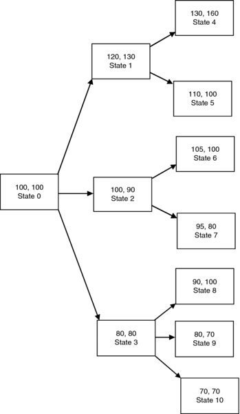
Figure 20.2 A finanical market with two risky assets
We will now describe the general discrete-time model. The notation is necessarily somewhat involved, but the market of Figure 20.2 is sufficient to capture the main ideas. We have a finite state stationary Markov chain (see Section 18.2) with the following special structure. The set of states is divided up into subsets ![]() , where
, where ![]() denotes the set of states at time k. There is a single state
denotes the set of states at time k. There is a single state ![]() reflecting the fact that there is no uncertainty about prices at time 0. The only transitions of positive probability are those from a state to another one which is one period later. That is, given states i in
reflecting the fact that there is no uncertainty about prices at time 0. The only transitions of positive probability are those from a state to another one which is one period later. That is, given states i in ![]() and j in
and j in ![]() where m is not k + 1, we must have pij = 0. For example, in our multi-period binomial model, there were k + 1 states at each time k, and for each state at time k, there were exactly two transitions into a state at time k + 1. In the market of Figure 20.2, we would have
where m is not k + 1, we must have pij = 0. For example, in our multi-period binomial model, there were k + 1 states at each time k, and for each state at time k, there were exactly two transitions into a state at time k + 1. In the market of Figure 20.2, we would have ![]() ,
, ![]() ,
, ![]() .
.
In the binomial case, we described outcomes by sequences consisting of U and D. In the general case, where we can have more than two branches from a node, we need a somewhat different representation. The evolution of our system up to time k can be described by a sequence of states {s0, s1, …, sk} where each ![]() and
and ![]() for j < k. We will call such a sequence an admissiblek-sequence. We now take our sample space Ω to consist of all admissible N-sequences, and this is equipped with the probability measure P where for any admissible N sequence ω, we have P(ω) = ΠN − 1k = 0psk, sk + 1.
for j < k. We will call such a sequence an admissiblek-sequence. We now take our sample space Ω to consist of all admissible N-sequences, and this is equipped with the probability measure P where for any admissible N sequence ω, we have P(ω) = ΠN − 1k = 0psk, sk + 1.
As an example, in the market of Figure 20.2, Ω consists of the 7 elements {{0, 1, 4}, {0, 1, 5}, {0, 2, 6}, {0, 2, 7}, {0, 3, 8}, {0, 3, 9}, {0, 3, 10}}.
It is convenient to adopt the following notational device. For any admissible k-sequence ν with k < N we let v° denote the set of all ω ∈ Ω which extend ν. That is if v = s0, s1, …, sk, then
For example, in the market of Figure 20.2, {0, 3}° will denote the subset {{0, 3, 8}, {0, 3, 9}, {0, 3, 10}}.
We now want to capture formally the nature of quantities like asset prices or asset holdings at a certain time k. These are random before time k, but are then known with certainty at time k or later. For example, in the market of Figure 20.2, the price of asset 1 at time 1 is a random variable which is uncertain at time 0, but then is known precisely at time 1. So it will take the constant value of 120 on the set {0, 1}° = {{0, 1, 4}, {0, 1, 5}}. Similarly it will take the constant value of 100 on the set {0, 2}° and the constant value of 80 on the set {0, 3}°.
We handle this in general by the following definition.
Definition 20.5 For any integer k = 1, 2, …, N, a random variable V defined on Ω is said to be k-determined if V is constant on any set ν° where ν is an admissible k − sequence.
For a k-determined random variable V, we will write V(ν) to denote the constant value of V on the set ν°.
It follows from the definition that a k-determined random variable is also m-determined if m ⩾ k. This just reflects the fact that if we know something at time k, we will know it just as well at some later time.
Note that a 0-determined random variable is just a constant, since the only 0-admissible sequence is that with the single entry of s0 and s°0 is the entire set Ω.
Definition 20.6 For any random variable W, we define a k-determined random variable Ek(W) as follows. Suppose that the point ω ∈ ν°. That is, ν comprises the beginning k + 1 entries of ω. We then define
using the notation of (20.20).
So Ek(W) then just gives the expected value of W conditional on the first k-steps of the evolution.
It is clear from the definition that Ek(W) is k-determined. E0(W), being 0-determined, is a constant and just equal to the usual expected value E(W). Consider the other extreme where k = N. Then for any ω, the set ν° is the single point ω and E(W|ω) is just W(ω), showing that EN(W) = W. So as k increases, Ek(W) gives us more and more information about W until we reach time N and know W exactly.
Example 20.5 Consider Figure 20.2. Suppose that where there are two branches emanating from a node, the probability of an upward move is 2/3 and that of a downword move is 1/3, while in the case of three branches emanating from a node, each has probability 1/3. Describe the random variable E1(S1(2)).
Solution. Consider the set B = {0, 1}°, which consists of the two points, namely {0, 1, 4} that has probability 4/9 and {0, 1, 5} that has probability 2/9. We could calculate that the conditional probabilities given B are (4/9)/(6/9) = 2/3 for {0, 1, 4} and (2/9)(6/9) = 1/3 for {0, 1, 5}. Observe now that we did not have to do all of this calculation, since the tree-like structure makes it possible to read off these conditional probabilities from the future branches of the tree without worrying about the past. In this case, with only one future step, they are immediate. We then have that E1((S1(2)) takes the value of 2/3(130) + 1/3(110) = 123 1/3 on {0, 1, 4} and{0, 1, 5}. Similarly, it takes the value of 101 2/3 on {0, 2, 6} and {0, 2, 7} and the value of 80 on {0, 3, 8}, {0, 3, 9} and {0, 3, 10}.
To summarize, a financial market with M + 1 risky assets and of duration N is modelled by a Markov chain with the special structure as noted above, a probability measure on the set Ω of all paths from time 0 to time N, a risk-free interest rate r, and random variables Sj(n), j = 0, 1, …M, n = 0, 1, …, N, on Ω where each Sj(k) is k-determined. A trading strategy consists of a collection of random variables αj(n), j = 0, 1, …M, n = 0, 1, …N − 1 where each αj(k) is k-determined.
For an important application to follow, we now turn to the concept of a martingale introduced in Section 18.3, and look at conditions for this to occur in our present context. Fix a probability measure Q on Ω which is equivalent to P and let {Wn}, n = 0, 1, …, N be a sequence of random variables such that each Wk is k-determined We claim that this will be a martingale, provided
To see this, suppose that the above holds. Fix any k and a sequence of real numbers {w0, w1, …, wk}. Consider any set which has positive probability under Q and is of the form
Now by definition, membership in A is determined by what happens up to time k. If a sequence ω ∈ A, any sequence which has the same first k + 1 entries must also be in A. This implies that A must be the union of subsets of the form ν° for some k-admissible sequence ν. For any such ν, it follows from our hypothesis (20.11) that
and from (A.22), (applied to the sample sample space A with the conditional probability Q( · |A) we can conclude that
showing that the sequence is a martingale.
To apply this, refer again to Figure 20.2. Let Q be the probability measure which assigns 1/3 to each transition when there are three transitions out of a state and 1/2 to each transition when there are two. We can then see that the sequence of prices of asset 1 is a martingale under this measure, by simply verifying the condition (20.11) at each node. For example, at state 3, we have that the value of S1(1) = 80 and the value of E1(S1(2)) = (1/3)90 + (1/3)80 + (1/3)70 = 80. The same holds at all other states. Similarly, we can show that the same holds for S2(n), the sequence of prices of asset 2.
20.9 Arbitrage-free condition
To decide when a general financial market is arbitrage-free, directly from Definition 20.2, could be extremely complicated. We would have to consider all possible initial portfolios with value 0 and all possible self-financing trading strategies. Fortunately, there is often a faster way. Suppose we can find a probability measure Q, equivalent to P, such that for each asset i, the sequence {Si(n)} is a martingale under Q. Consider any self-financing trading strategy. At any time n, the portfolio has a value V(n). For each asset i, the expected value at time n + 1 will again be Si(n) and so the expected value of the portfolio before trading will be V(n). Since our trading strategy is self-financing, the expected value after trading will again be V(n). Since this is true for all possible values of the portfolio at time n, we must have that EQ[V(n + 1)] = EQ[V(n)]. (The subscript indicates that expectations are with respect to the probability measure Q.) Working inductively, we have that EQ[V(N)] = V(0) = 0. It is impossible for V(N) to be nonnegative for all outcomes, have a positive probability of being positive, and still have an expectation of 0, so we cannot have an arbitrage opportunity.
This seems like a nice simple answer but on the face of it there is a major problem. It is not reasonable to expect that our stochastic processes for stock prices are martingales, as we indicated in Section 18.3. In fact, the bank account, by definition, cannot be a martingale unless r = 0. So our result above may appear at first to be meaningless, but the following trick saves the day.
We do not have to measure our assets in terms of dollars. They can be expressed relative to some other asset. Define
That is, ![]() is the value of asset j at time n in terms of the bank account. We can think of
is the value of asset j at time n in terms of the bank account. We can think of ![]() as a discounted or present value, since it is what we would have to invest in our risk-free bank account in order to accumulate to Sj(n) at time n. It is a random variable rather than a number since Sj(n) is a random variable. The same argument we gave above clearly goes through if each
as a discounted or present value, since it is what we would have to invest in our risk-free bank account in order to accumulate to Sj(n) at time n. It is a random variable rather than a number since Sj(n) is a random variable. The same argument we gave above clearly goes through if each ![]() is a martingale. This is now possible since
is a martingale. This is now possible since ![]() takes a constant value of 1. We have therefore proved the ‘if’ direction of the following major result.
takes a constant value of 1. We have therefore proved the ‘if’ direction of the following major result.
Theorem 20.4 (The fundamental theorem of asset pricing) A financial market is arbitrage-free if and only if there is a probability measure Q on Ω which is equivalent to P, and for which ![]() is a martingale for j = 1, 2, …, M.
is a martingale for j = 1, 2, …, M.
A major example is the the multi-period binomial model, where the given risk-neutral measure satisfies the conditions of the above theorem, as we verify from Equation (20.20). Indeed, suppose that ![]() , so that S(k) = s(1 + r)k. Referring to Equation (20.20), for any ω ∈ Ω,
, so that S(k) = s(1 + r)k. Referring to Equation (20.20), for any ω ∈ Ω,
so that
As another application, we can conclude immediately from our observations in the preceding section that the market of Figure 20.2 is arbitrage-free when r = 0.
Note that the risk-neutral probability p that we gave in the one-period binomial market was the only possible value that would make ![]() a martingale, as shown by Equation (20.20). The terminology is carried over and any probability measure Q satisfying the conditions of Theorem 20.4 is known as a risk-neutral measure. The main conclusion of this section then is that usually the best way to show a given a given financial market is arbitrage-free is to show the existence of a risk-neutral measure.
a martingale, as shown by Equation (20.20). The terminology is carried over and any probability measure Q satisfying the conditions of Theorem 20.4 is known as a risk-neutral measure. The main conclusion of this section then is that usually the best way to show a given a given financial market is arbitrage-free is to show the existence of a risk-neutral measure.
The converse of the fundamental theorem will be proved in the following section.
20.10 Existence and uniqueness of risk-neutral measures
20.10.1 Linear algebra background
To complete our study of financial markets, we require a knowledge of some facts in linear algebra. We assume familiarity with the concept of a linear space (also known as a vector space) and linear subspaces. We also assume familiarity with the concepts of closed and bounded sets. Any basic text on multivariate calculus should contain the necessary details. The following is a brief review, adapted to our ultimate goals.
Consider in particular the vector space W consisting of all real-valued functions defined on some finite set S, with the operations of point-wise addition and scalar multiplication. This is an n-dimensional space where n is the number of points in S. We let 0 denote the function which takes the value 0 at each point of s. (The context should distinguish this from the number 0.) For any f, g in W, we have an inner product
A subset K of W is said to be convex if it contains the line segment joining any two of its points. That is, given f and g in K and and a scalar 0 < γ < 1, the function γf + (1 − γ)g is in K.
A hyperspace in W is a proper linear subspace of maximum dimension, that is one less than the dimension of the space. So for example, a hyperspace can be visualized in two-dimensional space as a line through the origin, or in three-dimensional space as a plane through the origin. We need the following two facts about hyperspaces. The first is a fairly standard result and not difficult to verify. The second is quite a bit more advanced.
- Any hyperspace H is determined by its so called orthogonal vector. That is, there is an element q ≠ 0 in W such that
The element q is unique up to a scalar multiple. In two or three dimensions, we can visualize it geometrically as a vector perpendicular to H.
- Let L be any linear subspace of W and let K be a closed and bounded convex set that does not intersect L. Then there a hyperspace H containing L such that K does not intersect H.
It is simple enough to visualize this geometrically in three-dimensional space. If a line does not intersect a closed and bounded convex set, we can find a plane containing the line which does not intersect the set. This of course does not hold if the set is not convex. Suppose that K is a doughnut-shaped region, and the line goes through the hole. Then any plane containing the line must intersect K.
20.10.2 The space of contingent claims
We return now to our model as described above and apply our linear algebra concepts. For a given financial market, define the following sets. Let
We can view this as the space of contingent claims, those payments at time N which are determined by the particular path. An important subspace of W is given by

So L is the subspace of all replicable claims as defined above in Section 20.5. It is a linear subspace since, given f and g in L, we can replicate f + g by just holding at each stage the sum of the holdings in the trading strategies replicating f and g, and we can similarly achieve any scalar multiple of f by multiplying our holdings by that scalar. Let
This easily seems to be a linear subspace of L. We let
which is a convex subset of W.
So a nice linear algebra definition for a financial market to be arbitrage-free is to simply say that L0 does not meet K. (Of course any nonzero, nonnegative function f in L0 represents an arbitrage opportunity, but an appropriate scalar multiple of such an f will be in K and also in the subspace L0. We also use the fact that our original probability measure P must take a positive value on each ω.)
To illustrate, Figure 20.3 gives a geometric picture of the one-period binomial market. Any contingent claim is represented by a point (f(U), f(D)) in the plane. The set K is the line segment joining the points (0, 1) and (1, 0). The subspace L0 is a proper subspace and therefore must be a line through the origin. In the arbitrage-free case, this line will have negative slope and not meet K. In the case of an arbitrage opportunity, L0 as represented by the dotted line, has a slope that is either nonnegative, or equal to ∞, and it must intersect K. The picture also makes it clear that L is the entire plane, as we noticed enough, since it a subspace that properly contains L0.
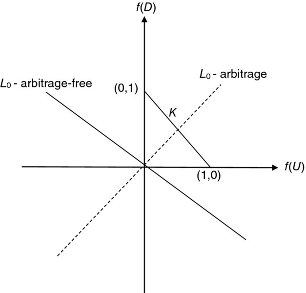
Figure 20.3 A picture of the one period binomial market
Further examples are furnished by the markets of Figures 20.4, 20.5 and 20.6. Assume that r = 0. Alternatively, we can assume any positive r and interpret the asset values that are given as as ![]() rather than Sj(n). The conclusions will be the same in either case.
rather than Sj(n). The conclusions will be the same in either case.
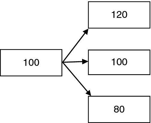
Figure 20.4 A market in which not all contingent claims are replicable
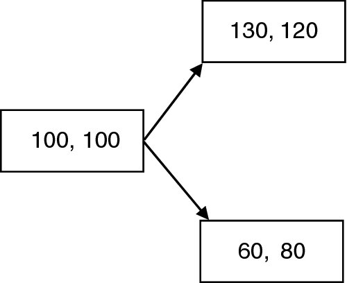
Figure 20.5 A market that is not arbitage-free
In the single risky asset market of Figure 20.4, the set Ω will have three points U, M, D (for ‘up’, ‘middle’, ‘down’). If the initial portfolio has α units of stock and β units of the bank account, the time 1 value of portfolio will be 120α + β for the upward movement, 100α + β if the price stays the same, or 80α + β for the downward movement. It follows that
a two-dimensional subspace of W, showing that not all contingent claims are replicable in this market. In particular, a call option with strike price 110 will have f(U) = 10, f(M) = f(D) = 0 which is not in L.
For initial portfolios of value 0, we must have in addition that 100α + β = 0 leading to
The intersection of L0 and K is clearly 0, showing that this market is arbitrage-free. Of course we could have immediately deduced this from the Fundamental Theorem, since assigning probabilities of 1/3 to each branch yields a risk-neutral measure.
Consider the two risky asset market of Figure 20.5. An initial portfolio with value 0 will be given by the vector of the form 100( − (α + β), α, β). Then, a function f will be in L0 if we can find α, β satisfying
These equations are readily solved to give α = −(f(U) + f(D))/10, β = (4f(U) + 3f(D)/20. It follows that L0 = L = W. So this market is about as far from being arbitrage-free as we could possibly get. Any contingent claim can be replicated for an initial cost of 0! Obviously, the prices here as shown could not be maintained by rational investors.
To see the delicacy of situations like this, look at this market again, but make the modification that S1(1) = 70 instead of 60. We leave to the reader to verify that we still have L = W, but L0 is quite different. The coefficient of α in the first equation of system (20.12) is 40 instead of 30, so that now
as in the market of Figure 20.3, which shows that the market is arbitrage-free. We can also deduce this immediately from the Fundamental Theorem, since now there is a risk-neutral measure, Q(U) = Q(D) = 1/2.
The market of Figure 20.2 that we investigated in Section 20.8 is more complicated, and it would involve a great deal of calculation to try to deduce L0 exactly, although we do know that it cannot meet K due to the arbitrage-free condition. It is possible to show that L = W, but this is far from obvious from the figures as given. As a particular case, consider the following.
Example 20.6 Let X be the contingent claim that that takes the value 60 on UU and 0 elsewhere. Take r = 0. Find a self-financing trading strategy to replicate this claim.
Solution. For any such strategy, each of the lower two nodes at time 1 will lead to a claim of 0 at time 2, so by the martingale property, our portfolio must have value 0 at these nodes. Therefore, looking at the pre-trading values at time 1,
which gives
Similarly, the value at the upper node at time 1 must be 60 times the probability of an upward move, which is 60(1/2) = 30. So
and substituting from above we have,
To summarize, the trading strategy at time 0 is to buy 1 unit of asset 2, financing this by selling 1/2 unit of asset 1, borrowing 40 and putting up the remaining 10. This checks out since the initial cost must be 60Q(UU) = 60(1/3)(1/2). At time 1, if the middle or lower branch occurs, sell the unit of asset 2, which is just enough to cover the short position and pay off the loan.
We must now decide what to do at time 1 if the upper branch occurs. In this case, we have
There are several solutions to these equations, which indicates that a replicating self-financing trading strategy need not be unique. One example is to take
This strategy involves borrowing an additional 60 to cover the short position in asset 1. At time 2, we pay off the loan of 100, and have either 60 or 0 left, depending on what happened to asset 2 at time 2.
Similarly, for each of the other six paths, we could find the replicating strategy for a claim which pays off only on that path. We would take a suitable linear combination of these seven strategies to replicate any possible contingent claim. This will show that L = W. In Section 20.11, we will prove a result which provides a much easier way to see this.
20.10.3 The Fundamental theorem of asset pricing completed
In this section, we prove the converse to the result established above, and show that in any arbitrage-free financial market, we can find a risk-neutral measure Q. We will proceed in two stages.
Stage 1: Defining Q:
By the arbitrage-free assumption, L0 does not meet the set K, a convex, closed and bounded set. By our linear algebra results of Section 20.10.1 we can find a hyperspace H containing L0 and not meeting K. Let q be an element orthogonal to H. That is H = {h: q · h = 0}.
Now it cannot be that for two distinct points f and g in K, we have q · f < 0 and q · g > 0, for if so we could find γ such that the function h = γf + (1 − γ)g satisfies q · h = 0 and so h ∈ H. But by convexity h ∈ K, and this would contradict the fact that H does not intersect K. So by a change of sign, if necessary, we can assume that q · f > 0 for all f ∈ K. Now in particular the functions 1ω which take the value of 1 on ω and the value 0 elsewhere are in K, and so we can infer that for all ω ∈ Ω,
and by multiplying by a suitable scalar we can ensure that
which means that the function q is the probability function for a probability measure Q on Ω.
Stage 2: Showing the martingale condition:
Fix any j. We will show that the stochastic process ![]() is a martingale under Q. For any time n < N and any possible value s of Sj(n), let A denote the event that Sj(n) = s, which means that
is a martingale under Q. For any time n < N and any possible value s of Sj(n), let A denote the event that Sj(n) = s, which means that ![]() .
.
We must show that
or equivalently that
where
Consider the following trading strategy. Do nothing before time n. If the price of asset j at time n is not equal to s, do nothing at all. If the price at that time is s, buy 1 unit of asset j, borrowing to do so, and sell it at time n + 1. Apply the proceeds to repaying the loan and let the difference (which could be negative) accumulate in the bank account. Let f be the function in W corresponding to this strategy.
If Sj(n) = s, this strategy yields a bank account of [Sj(n + 1) − s(1 + r)] at time n + 1. Multiplying by (1 + r)N − n − 1, the accumulated amount at time N is (1 + r)NY if the purchase is made and 0 if the purchase is not made. Our trading strategy is self-financing and requires an initial investment of 0. Therefore, the function g given by

is in L0. This means that
The fact that s is a possible value of Sj(n) implies that Q(A) > 0, and so we must have EQ(Y|A) = 0, establishing Equation (20.20).![]()
One method of showing that a market is not arbitrage-free is to find the subspace L0 and show that it intersects K. But as we saw above, this can be computationally infeasible in all but the simplest cases. The converse of the Fundamental Theorem provides an easier way.
Example 20.7 Use the above result to show that the financial market of Figure 20.5 is not arbitrage-free.
Solution. Given a probability measure on Ω, let q be the probability of an upward move. For ![]() to be a martingale, we need 130q + 60(1 − q) = 100 so that q = 4/7. For
to be a martingale, we need 130q + 60(1 − q) = 100 so that q = 4/7. For ![]() to be a martingale, we need that 120q + 80(1 − q) = 100 so that q = 1/2. No such measure exists.
to be a martingale, we need that 120q + 80(1 − q) = 100 so that q = 1/2. No such measure exists.
20.11 Completeness of markets
In this section, we pose the following questions. Given an arbitrage free market, can we price all contingent claims by the two methods we had in the binomial model? Can we do so uniquely?
The uniqueness question is easily answered for an arbitrage-free market. As we showed in the binomial case, if we can replicate a contingent claim with a self-financing trading strategy, then the cost of that claim should be the cost V(0) of setting up the initial portfolio. What happens, however, if there are several different replicating self-financing trading strategies? This can certainly occur, but in an arbitrage-free market, they necessarily have the same V(0) which means a unique price. Suppose to the contrary that there were two replicating strategies for the same contingent claim, one with an initial cost of 100 and the second with an initial cost of 60. The investor could follow both the second strategy and the reverse of the first strategy for a net gain of 40 at time 0 which would be placed in the bank account, resulting in an overall initial value of 0. At time N, the payments on these two strategies would cancel, leaving a certain positive amount in the bank account, contrary to the fact that there were no arbitrage opportunities.
We turn now to the existence question, beginning with a definition.
Definition 20.7 A financial market is said to be complete if, given any contingent claim X, there is a self-financing trading strategy that replicates X. In other words, using the notation of the preceding section, the subspace L is all of W.
We have already shown that the multi-period binomial market is complete. Moreover in Figure 20.4, we gave an example of an incomplete market.
The following theorem gives a characterization of completeness for arbitrage-free markets.
Theorem 20.5 An arbitrage-free market is complete if and only if there is a unique risk-neutral measure.
Proof. Suppose that the market is complete. Let Q be any risk-neutral measure. Fix any ω ∈ Ω. Let Xω be the contingent claim that pays 1 if ω occurs and pays 0 for all other outcomes, and choose a self-financing trading strategy that replicates Xω. If V(0) is the cost of the initial portfolio, the martingale property ensures that
so that
showing that Q is uniquely determined.
Conversely, suppose that the market is not complete, so that L is not equal to all of W. We can then choose a nonzero function h ∈ W such that
(Since we can do this for a hyperspace, we can clearly do it for any proper subspace which is contained in some hyperspace.) The function which takes the constant value 1 is in L, (achieved by investing (1 + r)− N in the bank account at time 0), so we must have that
Let Q be the probability measure with the probability function q as constructed in proving the ‘only if’ part of Theorem 20.4. We will produce a different function q′ with the same properties as q, namely
Then q′ will induce a second martingale measure Q′. To construct q′, we note that since q(ω) > 0 for all ω, we can choose a positive number δ sufficiently small so that the function
satisfies (20.20), and since h ≠ 0, q′ is different from q. In view of Equations (20.14) and (20.20), it is clear that q′ also satisfies Equations (20.17) and (20.20).
![]()
To illustrate the proof of the last part, look again at the market of Figure 20.3. The function q(ω) = 1/3 for all ω gives us a risk-neutral measure. The space L is, as we have seen, the set of all functions such that
and the perpendicular function h can be taken as
We can take then δ to be any number strictly between − 1/3 and 1/6, which yields an infinite number of risk-neutral measures.
As a consequence of the above theorem, we can see immediately that the market of Figure 20.2 is complete, without going through the somewhat involved calculation of the replications that we did before. The probability assignment which we gave in Section 20.8 is clearly the unique risk-neutral measure.
Incompleteness means that there are not sufficiently many assets to account for all the variations in possible contingent claims. Comparing Figures 20.4 and 20.5, we see that with three branches we need at least three assets in order to achieve completeness. This explains also the fact that with only one risky asset, we need a binomial model to achieve completeness.
For an additional example, consider the two risky asset market of Figure 20.5. We leave it to the reader to decide whether or not it is arbitrage-free, and whether or not it is complete.
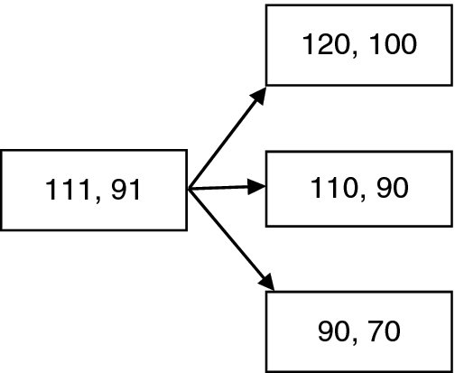
Figure 20.6 See Exercise 20.7
At this point, we summarize our conclusions. Suppose we have an arbitrage-free financial market. If the market is complete, then for any contingent claim X, there is a unique price which will prevent arbitrage opportunities. This can be found in one of two ways. First, choose a self-financing trading strategy to replicate X, and the price will be V(0). Second, take the discounted expected value of (1 + r)− NX with respect to the unique risk-neutral measure Q. If the market is incomplete, then we can still find a unique price for the replicable contingent claims. However the non-replicable claims cannot be priced uniquely, since different choices of a risk-neutral measure can give different results. Some other criteria must be used to arrive at prices. This does not mean of course that there are no restrictions on the price of such claims. Often, a range of values can be computed.
Example 20.8 In the market of Figure 20.4, find the possible no-arbitrage prices for a call option with exercise date 1 and strike price 110.
Solution. Add the option as another asset S2 with a price of π at time 0. For a martingale measure which has probability p of an upward movement and probability q of staying the same, we have 120p + 100q + 80(1 − p − q) = 100 implying that 2p + q = 1, so that p < 1/2. Applying the martingale condition for the new asset gives π = 10p, which means that we must have 0 < π < 5. Conversely, all such values are admissible since for any such π we obtain a martingale measure for the enlarged market by taking
In some cases, specifying the price of certain contingent claims will determine others. To illustrate, having added the additional asset and having specified π in Example 20.8, the resulting martingale measure is unique, so we have in effect completed the market. The price specified for the option will determine unique prices for all other contingent claims.
20.12 The Black–Scholes–Merton formula
The discrete-time model illustrates many of the fundamental principles of pricing contingent claims. There is a limitation, however. To be at all close to a realistic model, we would need an enormously large number of time periods and the computations will quickly become intractable. This is apparent just from looking at the cases for N = 2 of the previous section. For actual computation and greater realism, the preferred method is to use continuous-time models, which involve more advanced mathematical machinery. The relatively simple calculations effected by solving linear equations above will be replaced by solving differential equations. Sums of random variables are replaced by integrals of random variables, a concept that is technically very complex. The characterizations of arbitrage-freeness and completeness which we gave can be generalized to continuous-time settings but the proofs are far more difficult. A rigorous development of this is beyond the scope of the book, However we do want to investigate the Black–Scholes–Merton formula. This is a pivotal result which in fact initiated much of the modern research into stochastic models in finance.
In this section, it is convenient to use the risk-free force of interest δ = log (1 + r) instead of r.
We consider again the case of a financial market consisting of the bank account, and a single stock whose price at time t is S(t). The difference is that we now allow trading at any time, and moreover, we allow asset prices to vary continuously. We therefore must model S(t) as a continuous-time stochastic process and will in fact choose a geometric Brownian motion process, as given in Section 18.7. That is, for some constants μ and σ,
where B(t) is a standard Brownian motion.
The problem is to find the price of a European call option with exercise date N and strike price K. One approach is to make use of the results that we already know for the discrete-time model. Suppose we can find a probability measure Q under which ![]() is a martingale. Then we can approximate our process with our discrete time multiple period binomial model with periods of length 1/m,
is a martingale. Then we can approximate our process with our discrete time multiple period binomial model with periods of length 1/m, ![]() and with risk-free force of interest = δ/m, provided we take m sufficiently large. This should seem plausible since the log of our binomial process is a random walk. In this discrete setting, the price of the option is given in Equation (20.20). Putting in all the parameters and taking limits as m goes to ∞, we arrive at the celebrated Black–Scholes–Merton formula:
and with risk-free force of interest = δ/m, provided we take m sufficiently large. This should seem plausible since the log of our binomial process is a random walk. In this discrete setting, the price of the option is given in Equation (20.20). Putting in all the parameters and taking limits as m goes to ∞, we arrive at the celebrated Black–Scholes–Merton formula:
where
and Φ is the c.d.f. of the standard normal distribution. An alternative method to derive the formula is to directly calculate e− δNEQ[(S(N) − K)+]. This is more straightforward, involving basic calculus, although the calculation is somewhat involved. For both of these methods, we will omit the detailed derivations.
Note that the parameters to determine the option price are the risk-free force of interest δ, the strike price K, the duration N, and the quantity σ. The latter is a measure of the tendency for prices of the underlying stock to vary and is known as the volatility of the stock. Note however that the formula does not depend on μ. We comment more on this below.
The resulting formula seems somewhat formidable, but we can provide some motivation. The following is not intended as a rigorous exposition, but more to provide a method of remembering and understanding the structure of the formula. First consider the random variable
What is its distribution under Q? From the definition of Brownian motion, we know that under our original probability measure, it is normal with mean μN and variance σ2N. If we make the assumption that it is still normal under Q with the same variance, and calculate the resulting mean M, we know from Equation (A.58) that
But, since ![]() is a martingale with respect to Q,
is a martingale with respect to Q,
so that
leading to
We conclude that under Q, we have a new drift parameter (δ − σ2/2) which is completely independent of the original drift parameter μ. This is analogous to the observation in the simple one-period binomial model where the original probability played no role in the option price and it was only the risk-neutral probability that mattered.
Now let us ask, what is the probability under Q that the buyer of this option will exercise it? This will occur if S(N) > K. The probability of this is the same as the probability that X ⩾ log (K/S(0) which equals the probability that − X ⩽ log (S(0)/K), which by the results calculated above is
Given our above assumption regarding the distribution of X, we have now identified the term Φ(α) in the Black-Scholes-Merton formula as the probability under the risk-neutral measure that the option will be exercised.
Now consider the following rather naive reasoning to arrive at the option price. If we exercise the option, we will have an expected gain at time N of E[S(N) − K)] and this will have a present value of E[S(N) − K]e− δN. Multiply this by the probability of exercise to get
This looks something like the actual Black–Scholes–Merton formula, but unless σ = 0, the coefficient of S(0) differs. Our naive approach, however, ignores the nature of the option contract. With positive values of σ, the stock price at time N will vary, and could be above or below the exercise price. Calculating E(S(N) − K) will include negative values when the price is below K, but there is no loss in these cases since the option will not be exercised. The naive formula therefore understates the true price. Another way of expressing this is to note that what we really want is the expected value of S(N) − K, given that the option is exercised. To correct this understatement, it turns out that the coefficient of S(0) must be increased from Φ(α) to ![]() . This makes sense as we would expect that this correction should increase as the variability in the stock price and length of period increase.
. This makes sense as we would expect that this correction should increase as the variability in the stock price and length of period increase.
For further insight and verification, we can directly verify the formula for N = 0. In this case, Φ(α) = Φ( − ∞) = 0 if S(0) < K, and the formula gives an option price of 0, which it should, while Φ(α) = Φ(∞) = 1 if S(0) > K and the formula gives an option price of S(0) − K which it should.
There is still another important feature involving the two terms in the Black–Scholes –Merton formula, which we now present. Start with the following question. For the call option as above, what is its value at any time t, 0 ⩽ t ⩽ N? By the same argument as above, the value will be given by the same formulas as above except that in both (20.19) and (20.20), S(0) is replaced by by S(t) which is the stock price at time t and N is replaced by N − t, the remaining duration. It turns out that the two terms of this formula yield a replicating strategy for the option, and therefore a hedging strategy, in terms of holdings of the stock and the bank account. To explain this, we will take new units for the bank account, by adopting a slightly different but equivalent point of view, We can view the bank account as an investment in risk-free zero-coupon bonds maturing at time N. A unit of this asset will be a bond with face amount K, so that its value at time 0 = K(1 + r)− N. Let αt denote the value of (20.20) with S(0) replaced by S(t) and N replaced by N − t. The replicating trading strategy is to hold Φ(αt + σ(N − t)) units of the stock, and carry a short position of Φ(αt) units of the bonds we just described, at any time t. At each time t, the value of this portfolio will be precisely the value of the option as given above and it will reach the right amount at time N. In the case where the option is to be exercised the final portfolio will consist of 1 unit of stock, and a short position of 1 bond. In the other case, the portfolio will be reduced to zero units for both assets. It can be observed that the idea behind this strategy is similar to what we observed in the call option of Example 20.2, where the replication is accomplished by buying stock as the price increases, or selling as the price declines.
One must also show that this strategy is self-financing, using an appropriate modification of this definition to apply to continuous time. The idea is that at each instant, the amounts received from selling one of the assets is exactly what is required to buy the other. A precise definition is based on the formulation given in Exercise 20.3, with the differences replaced by differentials. This is not easy, however. The problem is that these are differentials of stochastic processes rather than deterministic functions, and a rigorous presentation involves some knowledge of the subject known as stochastic calculus.
Remark In real life of course this replication by continuous rebalancing is not possible. One could try to get close by very frequent rebalancing but there is no guarantee that this discrete-time approximation is self-financing. It could well require additional amounts of cash or release such. But one can hope that if our model is sufficiently accurate that these extra amounts are relatively small, so that the option could be replicated for something close to the Black–Scholes–Merton price.
To conclude this section, we note that while the Black–Scholes–Merton formula has persisted as the main tool for option pricing, it is based on several simplifying assumptions. One such assumption is that of the log-normal evolution of stock prices. There has been evidence to show that this is not completely realistic, and alternative models have been investigated. Another assumption is that both the risk-free force of interest and the volatility are constant and known, as these must be inserted into the formula to obtain numerical results. More realistic models have been proposed where these quantities are both considered as random.
20.13 Bond markets
20.13.1 Introduction
We now return to the discrete-time case. In this section, we deal with markets where the assets are risk-free zero-coupon bonds. These were already introduced in Section 2.12, where we considered forward prices, but here we want to consider the actual prices which will be random variables. A major result will be to give an appropriate version of 2.1 to ensure no arbitrage in the case of stochastic discount functions.
Our market will consist of N + 1 assets where for n ≠ 0, asset n is a zero-coupon bond maturing for 1 at time n. We will define S0 later.
We will denote the random variable Sk(n) by v(k, n). For k ⩽ n, v(k, n) is the price you would pay at time k to receive 1 at time n, which ties in well with our original use of this notation in Chapter 2, as well as our notation for forward prices. These are not the forward prices however, but the actual prices. Of course v(0, n) is a real number and the same as the forward price ![]() , since at time 0 we know the prices of the bonds. But future prices are unknown and therefore modelled as random variables.
, since at time 0 we know the prices of the bonds. But future prices are unknown and therefore modelled as random variables.
A question which may come to mind now is whether the fundamental Equation 2.1 could hold for these quantities only interpreted as a multiplication of random variables. The answer is no. Observe, for example, that with randomness
since the left side is a real number while the right side is truly random.
Now in order to avoid a completely trivial situation, we cannot assume a constant deterministic risk-free rate r as we did before. Before discussing how we modify this idea, we want to recall how risk arises from investment in risk-free assets like bonds, (elaborating on the discussion at the end of Section 2.10.3). Note first that unlike a stock, where a value on any future date is unknown, the payoff on a risk-free bond is absolutely certain if held to maturity. The risk arises if one wants to buy or sell before that date. For example, if the risk-free interest today is 5%, then the price of a 3-year bond will be (1.05)− 3 = 0.864. If at time 1, the risk-free interest rate has risen to 0.08, then the value of the bond drops to (1.08)− 2 = 0.857. Buying long-term bonds therefore carries the risk of a rise in interest rates, which can lower the price. However, in our present model, where trading occurs only at integer times, buying bonds which mature in 1 period does not carry any risk. This leads us to define the bank account by
Our bank account is formed by starting with 1 at time 0, using that to buy a bond maturing at time 1, then taking the proceeds of v(0, 1)− 1 to buy a bond maturing for v(0, 1)− 1v(1, 2)− 1 at time 2, and to continue rolling over the account into a new 1-year bond each year. In the case of a constant and deterministic interest rate of r, we would have v(k, k + 1) = (1 + r)− 1, and this definition of S0 reduces to the one given before.
Note that under this new definition, S0(k) is not a definite amount, but strictly random for k > 1.
Using the bank account, we can extend the definition of v(k, n) to all ordered pairs (k, n) by defining
since this is the amount accumulated at time k, by taking 1 from a bond maturing at time n and placing it in the bank account. Note that with this definition, all prices at the final time N are determined by the previous values of S0(n) (and of course the fact that V(N, N) = 1). This means that we can model our bond market with a tree going up to only time N − 1. (See Example 20.9 below.)
20.13.2 Extending the notion of conditional expectation
For our analysis, we will need some additional results about k-determined random variables, We will in fact investigate this idea in more generality and further extend the discussion in Section A.8, since the same ideas are needed in Chapter 24. Suppose we are given a sample space Ω, a probability measure P on Ω and a partition Π = {B1, B2, …Bn} of Ω into pairwise disjoint sets with union equal to all of Ω, such that for all i, P(Bi) > 0. For any random variable W on Ω, define a random variable ![]() as follows. For ω ∈ Bi,
as follows. For ω ∈ Bi,
To illustrate, in the model of Section 20.8, fix k and take the partition Π which consists of all sets ν° where ν is an admissible k sequence. (For example, in the market of Figure 20.2 if we take k = 1, the partition will consist of the three sets {0, 1}°, {0, 2}°, {0, 3}°.) Then ![]() is just Ek(W) as defined in that section.
is just Ek(W) as defined in that section.
We summarize the facts that we need in the following theorem.
Theorem 20.6 Take any random variables V, W and a scalar c.
(a) EΠ is linear. That is
(b) Suppose that W is a random variable which is constant on each subset of Π. Then
(c) Suppose that Π′ is a finer partition than Π which means that every set in Π is a union of sets in Π′. Then
Proof. (a) This follows directly by applying (A.23) and (A.8) to each subset Bi of the partition equipped with the probability measure P( · |Bi)
(b) As in (a) apply (A.8) to each set of the partition.
(c) It is clear from the definitions that if a random variable is constant on each subset of Π, then applying EΠ to it will leave it unchanged. Now EΠ(W) is constant on each subset of Π therefore constant on each subset of the finer partition Π′. It follows that ![]() . To show the other order of composition, choose any set A of the partition Π and let A be the union of sets B1, B2, …Bm where each Bi is a set of the partition Π′. To simplify the notation denote
. To show the other order of composition, choose any set A of the partition Π and let A be the union of sets B1, B2, …Bm where each Bi is a set of the partition Π′. To simplify the notation denote ![]() by Z. Now by definition, Z takes the constant value of E(W|Bi) on each set Bi so that clearly
by Z. Now by definition, Z takes the constant value of E(W|Bi) on each set Bi so that clearly
Now apply (A.29) to the sample space A equipped with the probability measure P( · |A). We have that
which shows that
![]()
It is of interest to look at the extreme cases. If we take Π to the finest possible partition where the sets are singletons, then EΠ(W) is just W. If we take Π to be the partition consisting of just one set, namely the whole space, which is the least fine partition, then ![]() is just the usual expectation E(W). The latter observation leads to some results of interest which we use in Chapter 24. Immediately from part (c) of the Theorem 20.6, for any W,
is just the usual expectation E(W). The latter observation leads to some results of interest which we use in Chapter 24. Immediately from part (c) of the Theorem 20.6, for any W,
More generally, if Z is any random variable which is constant on the sets of the partition Π, then from part (b) of Theorem 20.6
20.13.3 The arbitrage-free condition in the bond market
Return to our bond market with the assumption that for all k, the random variable v(k, n) is k-determined. What is the condition on v(k, n) to ensure that the market is arbitrage-free?
Lets go back to the deterministic setting of Chapter 2 for a moment. Note that if a special case of Equation (2.1) holds, namely
for all nonnegative integers k ⩽ n, then a straightforward induction argument shows that (2.1) will hold for all nonnegative integers k ⩽ m ⩽ n. (Example 20.9 below will make it clear why we begin with Equation (20.26) in place of the more general Equation (2.1))
We saw above that (2.1) does not hold when considered as a statement about random variables, but could it possibly be that this revised version will be valid? The answer is still no, since the left hand side is k-determined, but in general, since v(k + 1, m) is only k + 1-determined, the right side will only be k + 1-determined. It is plausible, however, that the following natural modification of our statement holds. Namely
It turns out in fact that Equation (20.27) is the correct condition to prevent arbitrage.
Theorem 20.7 If we can find a probability measure Q on Ω such that Equation (20.27) holds for all nonnegative integers k < n ⩽ N, then the given bond market is arbitrage-free.
Proof. We will show that under Q, each ![]() satisfies (20.11) and we can then apply Theorem 20.4. We know from the definition of S0 that
satisfies (20.11) and we can then apply Theorem 20.4. We know from the definition of S0 that
Moreover,
Now S0(k) is certainly a k-determined random variable, being a product of k-determined random variables, and so therefore is S0(k)− 1. Using Theorem 20.6(b) and invoking Equation (20.27)
completing the proof.
![]()
20.13.4 Short-rate modelling
We now deal with a problem that is different from that in previous sections. Instead of being given the asset prices, and asked if the market is arbitrage-fee or not, we are given some prices and want to determine other prices to satisfy the arbitrage-free condition.
For example, refer back to Equation (2.2). This shows in effect that in an deterministic setting, the prices for bonds of one period determine those for all periods. We do in fact have a stochastic version of this formula obtained by taking expectations.
Suppose we have a probability measure Q on Ω and random variables v(0, 1), v(1, 2), …v(N − 1, N), where v(k, k + 1) is k-determined. We extend this to all our prices by the rule that for k < n,
This will indeed result in an arbitrage-free market, since
establishing condition (20.20). Here we used the definition (20.28) in the first and last equality, For the second inequality we used Theorem 20.6(c) noting that for any k-admissible sequence ν, the set ν° is a disjoint union of sets ν°i where each νi is a k + 1-admissible sequence – simply add on all possible choices for the last element. So as k increases, the partitioning by k-admissible sequences gets finer. Finally, we use Theorem 20.6(b) for the third inequality.
Example 20.9 Take N = 3. As remarked above, we need only consider a two-period model. We will take the binomial model, and let Q be the probability measure that assigns equal probability of 1/4 to each of the four elements in Ω = {UU, UD, DU, DD}. Define the random variables v(0, 1), v(1, 2) and v(2, 3) by v(0, 1) = 0.7, v(1, 2)(U) = 0.8 v(1, 2)(D) = 0.6. v(2, 3)(UU) = 0.9, v(2, 3)(UD) = 0.7, v(2, 3)(DU) = 0.7, v(2, 3)(DD) = 0.5.
- Use (20.28) to find the distribution under Q of the other random variables v(k, n) for k < n, which will make the market arbitrage-free.
- Show that it is not necessarily true that v(k, n) = v(k, m)Ekv(m, n) if m ≠ k + 1.
Solution. (a) The other random variables are v(0, 2), v(0, 3), v(1, 3)which we will calculate directly from Equation (20.28)
The 2-determined random variable v(0, 1)v(1, 2)v(2, 3) takes the value of 0.7 × 0.8 × 0.9 on UU, the value of 0.7 × 0.6 × 0.7 on DU, the value of 0.7 × 0.8 × 0.7 on UD, and the value of 0.7 × 0.6 × 0.5 on DD. Each of these paths has probability 1/4, so
Now v(1, 2)v(2, 3) takes the value of 0.8 × 0.9 on UU and the value of 0.8 × 0.7 on UD so
Also, v(1, 2)v(2, 3) takes the value of 0.6 × 0.7 on DU and the value of 0.6 × 0.5 on DD so
(b) v(0, 2)E2[v(2, 3)] = (0.49)(0.7) = 0.343 ≠ v(0, 3)
To tie this example in with previous material, the reader may find it instructive to reproduce the figures shown in Figures 20.7 and 20.8. Figure 20.7 shows all the asset prices for all four assets, Figure 20.8 shows the values of ![]() for k = 1, 2, 3. The values of
for k = 1, 2, 3. The values of ![]() are of course all equal to 1.
are of course all equal to 1.
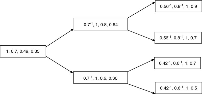
Figure 20.7 Example 20.9. Values of Sk(n), k = 0, 1, 2, 3
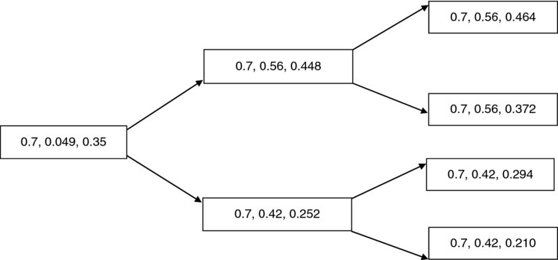
Figure 20.8 Example 20.9. Values of  , k = 1, 2, 3
Instead of specifying the one-period bond prices, we could equivalently have specified the interest rates as we did in Chapter 2, except that now ik = v(k, k + 1)− 1 − 1, which is a k-determined random variable.
We have shown that we can model stochastic interest rates in much the same way as we did in the deterministic model, that is, by choosing the one period rates first. For this reason, this procedure is sometimes referred to as short-rate modelling. What may be surprising at first, is that in the stochastic case the result in far from unique. We can indeed specify any probability measure we want for each ik, and achieve an arbitrage-free bond market. The procedure does not tell us how to choose the random variables ik and the probability measure Q. In practice, this can be motivated by trying to satisfy other conditions that one wants to impose. For example, at time 0, one knows the values v(0, n). But as we saw in Example 22.7, the values v(0, n) are determined from the one-period rates. A problem of some interest, which we will not deal with here, is to choose the distributions of the ik so as to recover specified values of v(0, n).
20.13.5 Forward prices and rates
We now expand on our definition of forward bond prices, which we introduced in Section 2.12
Suppose we are given a financial bond market as above. For j ⩽ k ⩽ n, we let
![]() = the forward price to be paid at time j for a 1-unit zero-coupon bond issued at time k and maturing at time n.
= the forward price to be paid at time j for a 1-unit zero-coupon bond issued at time k and maturing at time n.
This will be a j-determined random variable, since it is random depending on the state of nature up to time j. The quantity ![]() defined in Section 2.12 could be labeled as
defined in Section 2.12 could be labeled as ![]() .
.
The same argument as used in Section 2.12 shows that to prevent arbitrage, we must have
Indeed, if there is any sample point at which there is a discrepancy between these two random variables, an individual could wait and see if this particular sample point materialized at time j, which would be known by the fact that the random variables are j-determined. One could then follow one of two strategies, depending on which way the inequality went, to achieve a sure profit at time n.
In particular ![]() which is clear from the definition.
which is clear from the definition.
In place of the forward prices, we can describe the information available from the bond prices at time j by interest rates as we did before. For j ⩽ k, we define a j-determined random variable ij(k), the forward interest rate for contracts at time time j applicable to time period k to k + 1, by
Note that ik(k) = ik. In the deterministic case ij(k) = ik for all k.
It follows immediately from the definitions that
so that bond prices are determined by the forward interest rates. This suggests an alternative procedure to short-rate modelling for bond prices. The method is to model all the forward interest rates in place of the short rate ik. In this case, the forward rates at time 0 are all known, so the model will clearly reproduce the observed prices at time 0. One cannot, however, choose the distributions of the forward rates arbitrarily as for the short rates. Certain conditions must be imposed to ensure that the model is arbitrage-free. (See Exercise 20.12). This is another topic that is beyond our scope for further elaboration.
20.13.6 Observations on the continuous time bond market
We have concentrated on the discrete time setting for bond market, but many applications involve a continuous time framework. In this section, we give a very quick overview. It is intended mainly to bridge the gap and prepare those who wish to look at other sources and compare the material there with what we have done above.
Our market now will consist of zero-coupon bonds maturing at any time t, with a price at time s, of v(s, t). This will be a s-determined random variable under an appropriate extension of this definition to cover continuous time. As well we can define an extension of the conditional expectation Es. We will not go into details.
In place of the forward and spot rates of interest, one often wants to deal with the corresponding forces of interest, generalizing the quantity δ(t) to a stochastic setting. The forward force of interest, for contracts at time s applicable to time t is given by
an s-determined random variable.
In the deterministic case, when we can assume that our basic Equation (2.1) holds, then log (v(s, t) = log v(t) − log v(s) and all forward forces will be equal to δ(t) as defined in (8.8).
Knowing the forward forces determines bond prices uniquely, since by the definition
which we can view as a stochastic version of Equation (8.4) and as a continuous version of Equation (20.20).
We can also define a continuous and stochastic version of the short rate. Let δ(t) denote ![]() . This perhaps requires some care, since the partial derivative applies only to the second variable. Precisely
. This perhaps requires some care, since the partial derivative applies only to the second variable. Precisely
which will be a t determined random variable, and one which agrees with our Chapter 8 definition in the deterministic case. As in the discrete time case, this will not uniquely determine bond prices in a stochastic setting. Given any stochastic process for δ(t), we can produce an arbitrage-free bond market by taking
under a suitable interpretation of an integral of a random integrand.
Notes and references
This chapter constitutes a basic introduction to financial markets. For more comprehensive coverage of the basic concepts, see Hull (2014) or McDonald (2012). Readers particularly interested in the mathematics of continuous-time models can consult Björk (2009) or Etheridge (2002) for sources that are not overly advanced.
For many years, formula (20.19) was referred to as the Black–Scholes formula, recognizing the authors of the original paper that was published. Recently, many writers have added the name of Robert Merton, who made important contributions to developing and extending the ideas behind this result.
A proof of the extension result on hyperspaces can be found in Steland (2012), Theorem 2.4.5.
Those reading the financial literature should be aware that the terminology can differ from the actuarial conventions that we have adopted. Financial economists often use the word rate of interest to mean the continuously compounded rate, which we have called the force of interest.
Exercises
- 20.1 A one-period financial market has in addition to the bank account, one risky asset. The price at time 0 is 50, and at time 1, the price will either be 52 or 55 each with positive probability. For what value of the risk-free interest rate r will this market be arbitrage-free?
- 20.2 For the option contract introduced in Section 20.5, find an arbitrage opportunity if the option price is 11.
- 20.3 For the option contract introduced in Section 20.5, find the price if r is changed to (a) 11%, (b) 9 %. Can you explain why the prices change in this way?
- 20.4 Show that a trading strategy is self-financing if and only if, for 0 ⩽ n < N,
- 20.5 Assume the data of Example 20.2. Find the self-financing trading strategy for a 2-year American put option with a strike price of 106. Compare the price with the corresponding European put option.
- 20.6 Consider the financial market with N = 1, M = 1, r = 0, S1(0) = 100, S1(1) = 130, 110, or 80, all with positive probability.
- Find all possible risk-neutral probability measures.
- Consider a 1-year call option with a strike price of 100. (This is known as an ‘at-the-money’ option). Find the range of possible prices for this option that will avoid arbitrage.
- If the price of the option in part (b) is 12, find an arbitrage opportunity.
- 20.7 Consider the two risky asset market of Figure 20.6 with r = 0;
- Use Theorems 20.4 and 20.5 to decide whether or not this market is (i) arbitrage-free, (ii) complete.
- Describe the subspaces L and L0.
- 20.8 In Figure 20.3, find the slopes of the two lines representing L0 in terms of u, d and r.
- 20.9 When pricing options with the Black–Scholes–Merton formula, describe how option prices change, as changes occurs in volatility, strike price, duration, and risk-free force of interest. Use the formula and put-call parity to compute put and call prices for 3-month European options, on a stock selling now for 100 with a strike price of 110, 100 and 90 respectively, assuming σ is 0.2 and the force of interest for a 1-year period is 0.06. Verify your conclusions above by repeating the calculations for other values of σ, δ and duration.
- 20.10 For a certain stock, the price of a call option is 7.80 and the price of the corresponding put option with the same strike price and expiration date is 1.50. In each of the following scenarios, find the new price of the put option.
- A change in volatility raises the call price to 11.30.
- The stock price at time 0 is 100. A 10% increase in the strike price lowers the call price to 5.00.
- The risk-free force of interest is doubled and the time to expiration is cut in half, which combine to lower the call price to 7.00.
- 20.11 Consider a 6-month European call option on a stock now selling for 100, with a strike price of 97. You are given that σ = 0.25 and the force of interest for a 1-year period is 0.10. You would like to replicate this option by a trading strategy involving holdings in the stock and risk-free zero-coupon bonds of face amount 97, maturing in 6 months. You plan to use the Black–Scholes–Merton formula.
- What is the initial portfolio at time 0?
- At the end of 2 months, the stock price has risen to 105. What is your portfolio now?
- At the end of 4 months, the stock price has fallen to 95. What is your portfolio now?
- 20.12 Give a direct verification for the Black–Scholes–Merton formula in the case that σ = 0.
- 20.13 Verify directly from Figure 20.8 that the market of Example 20.9 is arbitrage-free and complete.
- 20.14 Redo Example 20.9 only assuming that the probability of an upward move is 3/4 and that of a downward move is 1/4.
- 20.15 A bond market has two transitions, U and D from time 0 to time 1. You are given the following forward prices:
 ;
; and
and  both take the value 0.8 on U and 0.6 on D.
- 20.16 Consider the bond market with prices as given in Figure 20.7. Consider a call option on a bond maturing for 1000 at time 3, with expiration date time 2. Find the price of the option if the strike price is (a) 900, (b) 650.
- *20.17 A universal life contract provides that your account will be credited with a minimum of 4% interest, up to a maximum of 10% interest. Describe the options present in this arrangement.