CHAPTER 4
Bonds
Bonds and debentures, which we have already introduced, are referred to as fixed-income securities. The reason is that once the rate of interest is set at the onset of the period for which it is due to be paid, it is not a function of the profitability of the firm. It is for this reason that all bonds—including floating-rate bonds, which entail the resetting of interest at the commencement of each interest-payment period—are referred to as fixed-income instruments. Interest payments are therefore contractual obligations, and failure to pay what was promised at the start of an interest-computation period will amount to default.
A bondholder is a stakeholder in a business but is not a part owner of the business. She is entitled to only the interest that was promised and to the repayment of principal at the time of maturity of the security and does not partake in the profits of the firm. As we discussed earlier, bonds may be unsecured or secured. Unsecured debt is referred to as a debenture in the United States, and the term connotes that no specific assets have been earmarked as collateral for the securities. In the case of secured debt, however, the issuer sets aside specific assets as collateral on which investors have a claim in the event of default. Debt securities may be negotiable or nonnegotiable. A negotiable security is one that can be traded in the secondary market, whereas a nonnegotiable security cannot be endorsed by the holder in favor of another investor. Bank accounts are classic examples of nonnegotiable securities, because if an investor were to open a term deposit with a commercial bank, although she can always withdraw the investment and pay a third party, she cannot transfer the ownership of the deposit.
The most basic form of a debt security is referred to as a plain vanilla bond. It is an IOU that promises to pay a fixed rate of interest every period, which is usually every six months in the United States, and to repay the principal at maturity. Floating-rate bonds are similar except that the interest rate does not remain constant from period to period but fluctuates with changes in the benchmark to which it is linked. There are also bonds with embedded options. Convertible bonds can be converted to shares of stock by the investor. Callable bonds can be prematurely retired by the issuing company, whereas putable bonds can be prematurely surrendered by the bondholders in return for the repayment of the principal. These bonds are discussed in greater detail later in the chapter.
Bonds provide equity shareholders with leverage. Here is a detailed illustration. Company ALPHA is entirely equity financed and has issued shares worth $1,000,000. Company BETA has raised the same amount of capital, half in the form of debt and the other half in the form of equity. The debt carries interest at the rate of 6 percent per annum.
Let us consider two situations. In the first, both companies make a profit of $250,000 from operations; in the second. they both make a loss of $250,000. To keep matters simple, we will assume that the firm does not have to pay tax.
From Table 4.1, the presence of debt in the capital structure creates leverage. The profit for the shareholders is magnified from 25 percent to 44 percent, when a firm is financed 50 percent with debt. On the other hand, the loss if incurred is also magnified, in this case from −25 percent to −56 percent. As we saw in the case of margin trading, leverage is a double-edged sword. It can also be seen from the case of BETA that the incurrence of a loss does not give the flexibility to the firm to avoid or postpone the interest due to bondholders. Interest on bonds is indeed a contractual obligation.
Bonds also provide the issuing firm with a tax shield because, although interest on debt is a deductible expense for figuring the tax liability of a company, dividends on equity shares are not. Interest payments reduce the tax liability for the firm or, in other words, give it a tax shield. Table 4.2 illustrates this using the same data as in Table 4.1. Both firms are assumed to have a profit of $250,000, and the applicable tax rate is assumed to be 30 percent.
Table 4.1 Illustration of Leverage
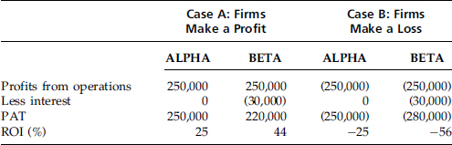
PAT stands for profit after tax and represents what the shareholders are entitled to. ROI is the return on investment for shareholders.
Table 4.2 Illustration of a Tax Shield
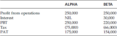
PBT stands for profits before tax; PAT stands for profits after tax.
Let us analyze the last row of Table 4.2. If company BETA had been a zero-debt company like ALPHA, its shareholders would have been entitled to an income of $175,000. However, because it has paid interest, the shareholders have received only $154,000, which is $21,000 less. From the standpoint of shareholders of BETA, they have effectively paid an interest of $21,000. So what explains the missing $9,000? After all, we know that BETA did pay $30,000 to its bondholders. The answer is that, by allowing the firm to deduct the interest paid as an expense before the computation of tax, the Internal Revenue Service (IRS) has forgone taxes to the extent of $9,000. The IRS has effectively provided a subsidy to the company. The tax shield, as we term it, is equal to the product of the tax rate and the interest paid. In this case, it is 0.30 × 30,000 = $9,000.
If the rules were to be amended and interest on debt were no longer to be tax deductible, BETA would have to pay tax on $250,000, and the profit after tax (PAT), which is what belongs to the shareholders, would be only $145,000. In this situation, the shareholders will feel the full burden of the interest paid by the firm.
In many countries, interest received from bonds is taxable at the hands of the receiver, whereas dividends received from shares are not. The reason is that because the interest is being paid out of pretax profits, it is not being taxed at the level of the firm. However, dividends on equity are not a tax-deductible expense for the firm; to prevent it from being taxed twice, it is not taxed at the hands of the shareholders.
Terms Used in the Bond Market
- Face value: Face value is also known as par value, redemption value, and maturity value.
- Principal value: Principal value is the principal amount underlying a bond. It was the amount raised by the issuer from the first holder, and it is the amount repayable by the issuer to the last holder. We will denote it by the symbol M.
- Term to maturity: Term to maturity is the time remaining in the life of a bond as measured at the point of evaluation. It may be perceived as the length of time after which the debt shall cease to exist and the point at which the borrower will redeem the issue by repaying the holder. Equivalently, it may be perceived as the length of time for which the borrower has to service the debt in the form of periodic interest payments. The words maturity, term, and term to maturity are used interchangeably. We will assume that we are stationed at time zero and will denote the point of maturity by T. The number of periods until maturity is T, which is normally measured in years.
- Coupon: The contractual interest payment made by the issuer is called a coupon payment. The name came about because in earlier days bonds were issued with a booklet of postdated coupons. On an interest-payment date, the holder was expected to detach the relevant coupon and claim his payment.
The coupon may be denoted as a rate or as a dollar value. We will denote the coupon rate by c. The dollar value, C, is therefore given by c × M. Most bonds pay interest on a semiannual basis, and the semiannual cash flow is c × M/2.
Consider a bond with a face value of $1,000 that pays a coupon of 8 percent per annum on a semiannual basis. The annual coupon rate is 0.08. The semiannual coupon payment is 0.08 × 1,000/2 = $40.
- Yield to maturity: Like the coupon rate, the yield to maturity (YTM) is also an interest rate. The difference is that although the coupon rate is the rate of interest paid by the issuer, the YTM is the rate of return required by the market. At a given point in time, the yield may be greater than, equal to, or less than the coupon rate. The YTM will be denoted by y, and it is the rate of return that a buyer will get if he were to acquire the bond at the prevailing price and hold it to maturity. We will shortly see that the YTM of a bond is equivalent to the concept of the internal rate of return (IRR) used in capital budgeting. As in the case of the IRR, the YTM computation assumes that all intermediate cash flows are reinvested in the YTM itself.
Valuation of a Bond
To value a bond, we will first assume that we are standing on a coupon payment date; that is, we will assume that a coupon has just been received and that the next coupon is exactly six months, or one period, away. If T is the term to maturity, we have N coupons remaining where N = 2T.
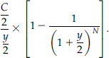
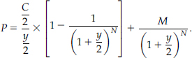
We will receive N payments during the life of the bond, where each payment or cash flow is equal to C/2. This payment stream constitutes an annuity. The present value of this annuity is
The terminal payment of the face value is a lump-sum payment. Because we are discounting the cash flows from the annuity on a semi-annual basis, this payment also needs to be discounted on a similar basis. The present value of this cash flow is

The price of the bond is therefore given by
As can be seen, the YTM is the discount rate that makes the present value of the cash flows from the bond equal to its price. The price of a bond is like the initial investment in a project. The remaining cash flows are similar to the inflows from the project. The YTM is exactly analogous to the IRR.
Example 4.1 demonstrates the valuation of a bond given the other variables.
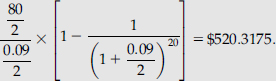
Infosys Technologies has issued bonds with 10 years to maturity and a face value of $1,000. The coupon rate is 8 percent per annum payable on a semiannual basis. If the required yield in the market is equal to 9 percent, what should be the price of the bond?
The periodic cash flow is 0.08 × 1,000/2 = $40. The present value of all the coupons is
The present value of the face value is
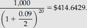
Therefore, the price of the bond is 520.3175 + 414.6429 = $934.9604.
Par, Premium, and Discount Bonds
In the preceding illustration, the price of the bond is less than its face value. Such bonds are said to be “trading at a discount to the par value” and are therefore referred to as discount bonds. If the price of the bond were to be greater than its face value, then it would be said to be “trading at a premium to its face value” and would be referred to as a premium bond. If the price is equal to the face value, then the bond is said to be trading at par.
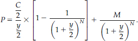
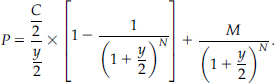
The relationship between the price and the face value depends on whether the YTM is greater or less than the coupon. Consider the pricing equation
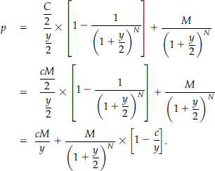
If c = y, P = M. In other words, if the coupon is equal to the YTM, the bond will always trade at par.
Let us differentiate the price with respect to the coupon.
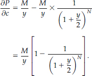
Price is a monotonically increasing function of the coupon. If the coupon is equal to the yield, then the price is equal to the face value. If the coupon is less than the yield, then the price will be less than the face value; if the coupon is greater than the yield, then the price will exceed the par value.1
Why would a bond sell at a premium or at a discount? The price of a bond is the present value of all the cash flows emanating from it. If the yield is equal to the coupon, then the rate of return being demanded by investors is exactly equal to the rate of return being offered by the issuer, and the bond will sell at par.
Suppose the yield is less than the coupon. Assume that the coupon is 10 percent per annum while the yield is 8 percent per annum. An investor will be willing to pay more than its face value for it. The price would be bid up to a level at which the YTM is exactly equal to 8 percent per annum. Finally, consider a case in which the YTM is greater than the coupon. Assume that the coupon is 8 percent per annum while the yield is 10 percent per annum. Investors in these circumstances will be willing to pay only a price that is less than the face value. The price would be driven down to a level at which the YTM is exactly equal to 10 percent.
Evolution of the Price
Let us consider the change in the price of a bond from one coupon date to another, assuming that the YTM remains constant.
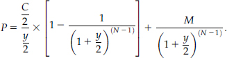
The price of a bond with N coupons remaining is
The price when there are N − 1 coupons left is given by
The price change between successive coupon periods is given by
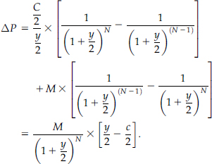
If y = c, then ΔP = 0. If the YTM were to remain constant, the price of a par bond would continue to remain at par, as we move from one coupon date to the next. If the yield is greater than the coupon, then ΔP > 0. A discount bond will steadily increase in price as we go from one coupon date to the next. In the case of a premium bond, the price will steadily decline as we go from one coupon date to the next.
Example 4.2 illustrates the change in the price from one coupon date to the next, keeping the yield constant, for both premium as well as discount bonds.
Consider a bond with 10 years to maturity and a face value of $1,000. Assume that the YTM is 8 percent per annum and the coupon is 6 percent per annum. The bond will sell at a discount. The price can be calculated to be $864.10. Let us move one period ahead to a time when only nine and a half years are left. The price can be calculated to be $868.66. As expected, the price has increased.
Consider the same bond but assume that the coupon is 10 percent per annum. The bond will sell at a premium. The price when there are 20 coupons left is $1,135.90. Six months later, if the yield were to remain constant, the price would be $1,131.34. As expected, the price has declined.
Zero-Coupon Bonds
Unlike a plain vanilla bond that pays coupons at periodic intervals, zero-coupon bonds, also known as deep discount bonds, do not pay any interest. Such instruments are always traded at a discount to the face value, and the holder at maturity will receive the face value. Consider a zero-coupon bond with a face value of $1,000 and 10 years to maturity. Assume that the required yield is 8 percent per annum. The price may be computed as follows:
![]()
Notice that we have chosen to discount at a rate of 4 percent for 20 half-yearly periods, and not at 8 percent for 10 annual periods. The reason is that a potential investor will have a choice between plain vanilla bonds and zero-coupon bonds. To draw meaningful inferences, it is imperative that the discounting technique be common. Because the cash flows from plain vanilla bonds are usually discounted on a semiannual basis, we choose to do the same for zero-coupon bonds.
A zero-coupon bond will never sell at a premium. It will always trade at a discount except at the time of maturity when it will trade for the face value. That does not mean that a buyer of such a bond will always experience a capital gain. If she were to buy and hold it to maturity, then she will have a capital gain. But if she chooses to sell it before maturity, she may well end up with a capital loss as we shall demonstrate in Example 4.3.
Alexis bought a zero-coupon bond when there were 10 years to maturity. The prevailing yield was 10 percent per annum. Today, a year later, the YTM is 12 percent per annum. The purchase price was ![]() . The price at the time of sale can be shown to be $350.34. In this case, the investor has a capital loss of $26.55.
. The price at the time of sale can be shown to be $350.34. In this case, the investor has a capital loss of $26.55.
Valuing a Bond in between Coupon Dates
We have assumed that we are valuing the bond on a coupon date—that is, the next coupon is exactly one period away. Let us consider a more realistic situation in which the price of the bond is to be calculated between coupon dates.
Consider the timeline depicted in Figure 4.1.
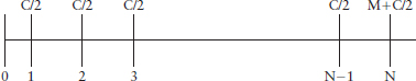
Figure 4.1 Cash Flows from a Plain Vanilla Bond
As you can see, the length of time between 0 and 1 is less than one period, whereas the other coupon dates are spaced exactly one period apart.
To value the bond at time 0, we will proceed in two steps. First, let us value the bond at time 1. At this point in time, we will get a cash flow of C/2. There are N − 1 coupons left after this, and the face value is scheduled to be received N − 1 periods later. The present value of the remaining cash flows at this point in time is
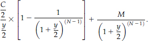
The price of the bond at time ‘1’ is
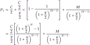
Let us denote the length of time between 0 and 1 by the symbol k where, k < 1. Discounting back P1 for k periods, we get

Day-Count Conventions
When valuing a bond between coupon dates the key issue is the calculation of the fractional first period. Unfortunately, there is no unique method for computing this period. Different markets, and at times different products in the same market, follow different conventions. A method of computation of the fractional period is called a day-count convention.
Actual–Actual
We will illustrate a convention known as the actual–actual approach. This is used for Treasury bonds in the United States. Let us go back and analyze the fractional period. To compute the fraction, we need to define the numerator and the denominator. The numerator is the number of days between the valuation date and the next coupon date. The denominator is the number of days between the previous coupon date and the next coupon date.
With the actual–actual method, we have to count the exact number of days in both the numerator and the denominator. We will illustrate it with the help of Example 4.4.
Let us assume that we are standing on May 21, 20XX, and that we have bond maturing on May 15 (20XX + 20). The face value is $1,000, the coupon rate is 6 percent per annum payable semi-annually, and the YTM is 8 percent per annum. The coupon dates are May 15 and November 15.
The numerator in this case is the period between May 21 and November 15. The number of days is calculated monthwise as shown in Table 4.3. The principle is that we include either a starting date or an ending date, but not both.
Table 4.3 Calculation of the Numerator
| Month | Number of Days |
| May | 10 |
| June | 30 |
| July | 31 |
| August | 31 |
| September | 30 |
| October | 31 |
| November | 15 |
| Total | 178 |
The denominator is the period between May 15 and November 15. In this case, it is 184 days as shown in Table 4.4.
If we were to count the actual number of days between two dates, which are six months apart, we will always get a number between 181 and 184. There are only four possibilities: 181, 182, 183, and 184.
Table 4.4 Calculation of the Denominator
| Month | Number of Days |
| May | 16 |
| June | 30 |
| July | 31 |
| August | 31 |
| September | 30 |
| October | 31 |
| November | 15 |
| Total | 184 |
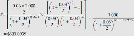
The actual–actual method is denoted in short form as Act/Act and is pronounced as “ack–ack” by Wall Street traders. Let us use it to derive the price of the bond on May 21, 20XX. The number of coupons remaining as of this day is 40. The value of the fractional first period is 178/184 = 0.9674.
The price of the bond is therefore:
The Treasury's Approach
The Treasury uses a slightly different method to compute the prices of its bonds, with the difference being that it uses simple interest for the fractional period. The Treasury's formula may be stated as
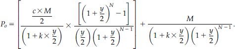
In this case, the price obtained by the Treasury will be $803.0738. The price that is computed by the Treasury for a given bond will always be lower than the value determined by Wall Street. This is because simple interest gives a higher discount rate for fractional periods as compared to compound interest.
Corporate Bonds
Corporate bonds in the United States are priced using a different day-count convention known as 30/360 PSA. In accordance with this convention, the denominator or the time period between two successive coupon dates is always taken to be 180 days—that is, every month is assumed to consist of 30 days. To compute the fractional period, the numerator is determined as follows.
Let us define the start date as D1 = (month1, day1, year1) and the end date as D2 = (month2, day2, year2). The numerator is calculated as
![]()
Some additional rules may have to be applied, depending on the circumstances.
- If day1 = 31, then set it equal to 30.
- If day1 is the last day of February, whether 28 or 29, then set it equal to 30.
- If day1 is 30 or it has been set equal to 30 based on the two rules listed above, then if day2 = 31, set it equal to 30.
Let us take the case of the bond maturing on May 15 (20XX+20). The valuation date as per our assumption is May 21, 20XX. The numerator for the fractional period is given by
![]()
The value of the fractional period is 174/180 = 0.9667.
The value of the bond is therefore
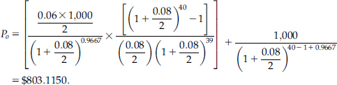
The day-count convention does have an impact, albeit a minor one, on the price.
Accrued Interest
The value of the bond as calculated by us using the appropriate day-count convention is referred to as the full or the dirty price. This is the price that is payable by the buyer to the seller. The price includes a component called the accrued interest, which we will explain.
When a bond is sold between two coupon dates, the next coupon will go to the buyer of the bond. However, because the seller has held the security for a fraction of the coupon period, he is entitled to a part of the next coupon payment. This fraction of the next coupon that belongs to the seller is termed the accrued interest. The bond-pricing equation that we used earlier automatically factors in the accrued interest, because it discounts all the forthcoming cash flows, from the perspective of the buyer, until the date of sale. The partial derivative of the dirty price with respect to the length of the fractional period is negative. The shorter the time remaining until the next coupon, the higher the accrued interest, keeping all other variables constant, and hence the higher is the dirty price.
The method for computing the accrued interest is a function of the day-count function. Let us take the case of the Treasury bond. On May 21, 20XX, it has accrued interest for 6 days. The total length of the coupon period is 184 days.2
The accrued interest is therefore
![]()
The dirty price minus the accrued interest is referred to as the clean price. In this case, it is $803.0939 − 0.9783 = $802.1156.
The significance of the clean price may be demonstrated as follows. Consider the value of the bond on the previous coupon date—that is, May 15, 20XX—assuming that the YTM is 8 percent per annum. The price comes out to be $802.0722.
On May 15, there is no difference between the clean price and the dirty price, because interest accrual for the next period is yet to commence. If the YTM is assumed to be constant, then the dirty price changes by $0.9783, which amounts to almost a dollar, whereas the clean price changes only by $0.0434. In the absence of a change in yield, the clean price remains relatively constant in the short run.
Look at the situation from the perspective of a bond-market analyst. She knows that yield changes induce price changes. However, if she were to analyze dirty prices, she would be unable to discern how much of the perceived change is the result of a movement in the required yield, and what is resulting from the change in accrued interest. Analysts look at prices that are not contaminated with accrued interest, or what we term clean prices. For this reason, quoted prices in bond markets are always clean prices. However, a trader who buys a bond has to pay the full price or the dirty price. When a bond is bought, the accrued interest has to be computed and added to the quoted price in order to determine the amount payable.
Negative Accrued Interest
One interesting question is, can the accrued interest be negative? Let us analyze the possible reason why the accrued interest may be negative. Accrued interest represents the amount that the seller of the bond is entitled to by virtue of the fact that he has held the bond for a part of the coupon period. The buyer has to compensate him with this amount. Negative accrued interest would correspond to a situation in which the seller has to compensate the buyer, and such a case can arise when the bond trades ex-dividend.
Certain bonds trade on an ex-dividend basis close to the coupon date. We know that bonds pay coupons and not dividends, and the term ex-dividend is a bit of a misnomer. However the implication is the same. Until the ex-dividend day, a bond will trade cum-dividend—that is, the buyer will be entitled to the next coupon. On the ex-dividend day, however, the bond will begin to trade ex-dividend, which implies that the next coupon will go to the seller and not the buyer. But from the perspective of a buyer who acquires the bond on or after the ex-dividend day, he is entitled to the pro rata interest for the number of days remaining until the next coupon date. In such a situation the seller has to share a part of the interest received with the buyer, which leads to a situation in which the accrued interest is negative.
Let us consider a corporate bond maturing on May 15 (20XX+120). Assume that we are on November 8, 20XX, which is an ex-dividend date. The dirty price just before the bond goes ex-dividend is

The moment the bond goes ex-dividend, the price will drop by the present value of the next coupon because the buyer is no longer entitled to it. The ex-dividend dirty price is
![]()
Notice that the dirty price will fall by the present value of the coupon and not by the coupon itself. This is because there is a week remaining until the next coupon, so we need to discount the cash flow.
The accrued interest as of November 8, 20XX, is
![]()
The ex-dividend clean price is 832.9078 − 28.8587 = $804.0491. The ex-dividend clean price is greater than the ex-dividend dirty price by $1.0966. This is the negative accrued interest, and it corresponds to the accrued interest for the remaining week, which is
![]()
Yields
The yield or the rate of return from a bond can be computed in a variety of ways. We have already referred to the YTM, which we will discuss in further detail shortly. We will also examine a number of other yield measures.
The Current Yield
The current yield is very simple to compute, although technically it leaves a lot to be desired. However, it is commonly reported in practice, because of the ease with which it can be calculated.
To compute the current yield, we simply take the annual coupon payment (irrespective of the frequency with which the coupon is paid) and divide it by the current market price. Thus,
![]()
One question is, should the price used be the clean or the dirty price? If the clean price were to be used, then the current yield would change only when there is a change in the YTM. However, if the dirty price were to be used, the current yield using the dirty price would be lower than the value obtained using the clean price if we were to calculate it before the ex-dividend date. This is because the dirty price in this period will be higher than the clean price. Besides, even if the YTM were to remain constant, the current yield will steadily decline along with the increase in the dirty price. In the ex-dividend period, however, the value of the current yield that we get with the dirty price will be higher than what we would get with the clean price because the dirty price will be lower than the clean price. In this period, too, if the YTM were to remain constant, the dirty price would steadily increase, and the current yield would steadily decline. If we were to plot the current yield versus the dirty price, for a given YTM, we would get a saw-tooth pattern.
Why do we say that the current yield is an unsatisfactory yield measure? Consider the case of an investor who has a one-year investment horizon. She will get a coupon of $C in the course of the year. If we assume that P0 was the price she paid at the outset to acquire the bond, then her interest yield for the year is the same as the current yield as defined by us. But even if this investor were to have a one-year horizon, she will sell the bond at the end of the year, unless, of course, it were to mature at that time. She will experience a capital gain or a loss.3
If the investor were to have a longer-term horizon, she will get additional coupons. These can be reinvested to earn income. Besides, when multiple cash flows are involved, the time value of money will enter the picture. All these facets of yield computation are totally ignored by the current yield measure.
Example 4.5 illustrates how the current yield is computed.
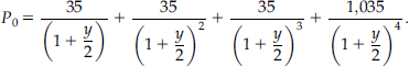
Consider a bond with a face value of $1,000 and a coupon of 8 percent per annum payable semiannually. Assume that the current price is $950.
The annual coupon is $80. The current yield = 80/950 = 0.084211 ≡ 8.4211%.
Simple Yield to Maturity
The simple yield to maturity, also known as the Japanese yield because it is a key yield measure used in Japan, factors in the capital gain or loss that an investor will get. However, it assumes that the bond will be held to maturity and that capital gains and losses occur evenly over the life of the bond. In other words, it builds in the assumption that capital gains and losses occur on a straight-line basis.
Consider the case of an investor who buys the bond at a price P. If he holds it to maturity, he will get back the face value, M. The capital gain or loss over the investment horizon is given by M − P. If the bond is bought at a discount, there will be a capital gain; if it is bought at a premium, there will be a capital loss. If we assume that we are standing on a coupon date and that there are N coupons left, then there are N/2 years remaining until maturity. The capital gain or loss amortized on a straight-line basis is

The simple YTM is given by
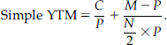
One shortcoming of the Japanese yield is that it fails to take into account the fact that investors in bonds can reinvest the coupons received by them in order to earn interest on such interest. This has the potential to significantly increase the returns from holding a bond, as we shall demonstrate in Example 4.6.
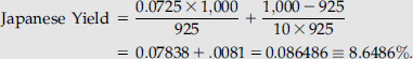
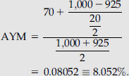
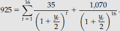
Consider a bond with a face value of $1,000 that pays coupons at the rate of 7.25 percent per annum. Assume that the current price is $925 and that there are 10 years to maturity. The Japanese yield is given by
Yield to Maturity
The yield to maturity is the internal rate of return of a bond. It is that single discount rate4 that makes the present value of the cash flows from a bond equal to its price. The bond-pricing equation is a nonlinear equation. Because there is only a single change of sign in the cash flows, from Descartes' rule of signs we know that there will be a single positive real root. The pricing formula gives us a polynomial of degree N, assuming that the bond has N coupons remaining. To solve it, we require a computer program in general, although we can get fairly close with the approximate yield to maturity (AYM) approach, which we shall demonstrate. We will show subsequently that it is a very simple matter to compute the YTM for zero-coupon bonds and bonds with only two coupons remaining.
Approximate Yield to Maturity
Consider a bond with a face value of M, a current price of P, an annual coupon of C, and N coupons remaining until maturity.
The current investment in the bond is $P. An instant before the bond matures, the investment in the security is $M. The average investment is (M + P) ÷ 2.
The annual capital gain or loss computed by amortizing on a straight-line basis is
![]()
as we have seen in the case of the Japanese yield.
The approximate YTM is defined as
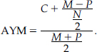
The numerator in the expression represents the annual income for the investor, assuming, of course, that capital gains or losses are realized on a straight-line basis. As we have explained, the denominator is the average investment during the life of the bond.
Once the approximate yield is computed, we need to choose an interest-rate band such that the upper limit gives a lower price than the observed price, whereas the lower limit gives a higher price. The exact YTM is then obtained using linear interpolation.
Example 4.7 demonstrates the computation of the yield to maturity using an approximate value followed by interpolation.
Consider a bond with a price of $925. The coupon is 7 percent per annum, and the face value is $1,000. There are 10 years to maturity, and the bond pays coupons on a semiannual basis.
Let us choose a band of 7.75−8.25 percent. The prices at the two extremes are 948.4675 and 915.9929. In this case, the actual price lies between the two extreme prices. However, at times we may end up choosing the interest-rate band in such a way that the actual price is either higher than both the extreme values or is lower than both. In such cases, we have to redefine the band such that one of the corresponding prices is higher than the actual price while the other is lower.
Let us interpolate. 8.25−7.75 percent corresponds to a price difference of 915.9929 − 948.4675. So, 8.25% − y* should correspond to a price difference of 915.9929 − 925, where y* is the true YTM.
![]()
If we take the ratio of both and solve for y*, we get
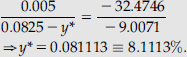
We can calculate the price corresponding to a YTM of 8.1113 percent to verify the accuracy. It comes out to be $924.86.
Zero-Coupon Bonds and the YTM
It is a very simple task to determine the YTM for a zero-coupon bond given its price, as the following example will illustrate.
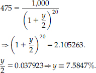
Consider a bond with 10 years to maturity and a face value of $1,000. Assume that the current price is $475. The pricing equation is5
Analyzing the YTM
To better appreciate the mathematics underlying the YTM, let us consider the sources of return for an investor who buys the bond at the prevailing market price and holds it to maturity.
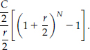
She will get N coupons, with each coupon equal to $C/2. Each time she gets a coupon, she can reinvest at the market yield prevailing at that time in an asset of the same risk class. And, finally, when the bond matures, she will be repaid the face value. The cash flows from the coupon payments constitute an annuity. When these cash flows are reinvested, they will earn interest. The important thing is the future value of these cash flows at the time the bond matures, which can be computed by using the standard annuity formula. Let us assume that each cash flow can be reinvested at a periodic (six-monthly) rate of r/2 percent. For ease of exposition. we will assume that r is the same for each cash flow or, in other words, that the reinvestment rate is a constant. This is not a necessary assumption and is made purely to facilitate the presentation of the argument.
The future value of the coupons as calculated at the time of maturity is given by
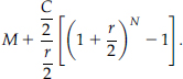
The total cash flow at maturity is
From the bond-pricing equation
When can we make a claim that we have received a yield of y/2 per period over N periods? Only if the terminal cash flow is equal to the initial investment compounded at y/2 for N periods.
In other words, we can claim that we have obtained a semiannual yield of y/2 if
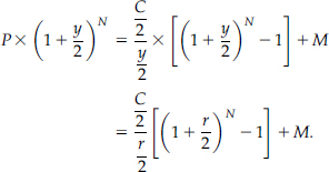
The implication is that to receive a periodic yield of y/2 over N periods, we need to satisfy two conditions. First, the investor must hold the bond until the maturity date. Second, y/2 must equal r/2. In other words, each intermediate cash flow obtained during the life of the bond (coupon) must be reinvested at the YTM prevailing at the time of acquisition of the bond.
Let us analyze the consequences of relaxing this assumption.
The Realized Compound Yield
We will relax one of the two preceding assumptions. Although we will continue to assume that the bond continues to be held until maturity, we will no longer take it for granted that each coupon is reinvested at the YTM. Instead, we will assume a specific rate r at which the coupons are assumed to be reinvested.
Example 4.8 illustrates the approach adopted to compute what is termed the realized compound yield.
Consider the bond with a face value of $1,000 and 10 years to maturity. The price is $925, and the coupon is 7 percent per annum paid semiannually. The YTM obtained by us was 8.1113 percent.
Assume that each cash flow can be reinvested at 7 percent per annum, or at 3.50 percent per six-month period.
The future value of the coupons is
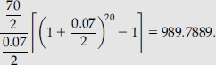
The terminal cash flow is 1,000 + 989.7889 = $1,989.7889.
The initial investment was $925. The rate of return over 20 periods is given by
![]()
This return is called the realized compound yield. It can be done on an ex-ante basis, as we have just done, by assuming a rate at which the reinvestment will take place, or on an ex-post basis by plugging in the actual rate at which the cash flows were reinvested.
In this illustration, the realized compound yield is less than the YTM because the reinvestment rate assumed by us is less than the YTM. If we had assumed a reinvestment rate higher than the YTM, we would have obtained an RCY greater than the YTM.
Reinvestment and Zero-Coupon Bonds
The inability to reinvest at a rate of return assumed at the outset is referred to as reinvestment risk. For coupon-paying bonds, reinvestment risk is a critical feature. Zero-coupon bonds are devoid of reinvestment risk for there are no coupons to be reinvested. To obtain a rate of return equal to the YTM for a zero-coupon bond, we have to satisfy only one condition: we should hold the bond to maturity.
The Holding-Period Yield
We will relax both the assumptions that we made earlier in order to compute the YTM. The first change, as we did in the case of the RCY, is that we will explicitly assume a rate at which the coupons are reinvested. Second, we will no longer assume that the bond is held to maturity but will assume an investment horizon that is shorter than the time to maturity. The corresponding yield measure is termed the horizon yield or holding-period yield.
The consequence of the second assumption is that it is no longer necessary for an investor to receive the face value at the end of his investment horizon. He will receive the market price at that time, which may be more or less than the face value and will depend on the YTM prevailing at that time.
Because we need to compute the sale price before maturity, we need to make an assumption about the YTM that is likely to prevail at that time, if we are computing the holding period yield on an ex-ante basis.6
Let us consider the data that we used to compute the RCY. However, we will assume that the investor has a horizon of eight years or 16 semiannual periods. We will assume that the bond can be sold at a YTM of 7.50 percent at the end of eight years. At that point in time, it will be a two-year bond. The corresponding price is $990.8715.
The future value of the reinvested coupons is given by7
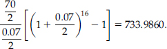
The terminal cash flow is 990.8715 + 733.9860 = 1,724.8575.
The rate of return over the eight year period is given by
![]()
Taxable-Equivalent Yield
Certain bonds are exempt from income taxes. In the United States, both the federal and state governments are empowered to levy such taxes. To deal with a situation in which a comparison is sought between a bond with taxable interest and another with tax-free income, we need to compute the taxable-equivalent yield (TEY) of the tax-free bond.
The computation of the TEY depends on the applicable taxes. Let us first consider a municipal bond that gives a yield of 6.00 percent. The bond is exempt from federal income tax, which we will assume to be 25 percent. The TEY is given by
![]()
The implication is that an investor should be indifferent between a taxable bond that yields 8 percent and the tax-free municipal bond, which yields 6 percent. If the taxable bond were to yield more than 8 percent, he would prefer it. On the other hand, if it were to yield less than 8 percent, he would prefer the municipal bond.
To make the computation more precise, we need to account for the fact that both bonds attract state income tax. This per se does not warrant an adjustment, because both the bonds will be equally impacted. However, for a bond that attracts both federal and state income taxes, the state tax can be deducted from the federal tax bill. This calls for the following adjustment.
Let us assume that the federal rate is 25 percent while the state tax rate is 8 percent. The adjusted federal rate is given by
![]()
The TEY of the municipal bond is therefore
![]()
The rationale for this correction is the following. If a person were to earn $100 of income, he will have to pay $8 by way of state tax. The federal tax is applicable only on $92. So the effective federal tax rate is: 0.92 × 0.25 = 0.23 ≡ 23%.
Consider the municipal bond is exempt from both federal and state taxes. To make the necessary adjustment, we need to compute the combined tax rate for a bond that is subject to both taxes. In our case, it is 23% + 8% = 31%.
The TEY of the municipal bond in such a situation is given by
![]()
There can be a situation in which the taxable bond that is being compared with the municipal bond is subject to federal taxes but not to state taxes. If so, we need to compute the TEY of the taxable bond and compare it with that of the municipal bond.
Assume that a T-bond with a coupon of 6.90 percent is being compared with a municipal bond that is exempt from both state and federal taxes. The TEY of the T-bond is
![]()
This TEY should be compared with the TEY of the municipal bond, and the bond that offers the higher TEY will be deemed to be superior.
Credit Risk
Credit or default risk is the risk that the coupons or principal or both may not be paid as scheduled. Except for Treasury securities, which are backed by the full faith and credit of the federal government, all debt securities are subject to default risk and differ only with respect to the degree of the associated risk. When a bond is issued, the borrower will release a prospectus with detailed information about its financial health and credit-worthiness. However, most investors lack the required skill sets to draw meaningful conclusions from analyzing such documents. To give confidence to potential investors about the quality of the issue, issuers get the securities rated by credit-rating agencies. These agencies specialize in evaluating the credit quality of a security issue. They not only provide a rating before the issue but also continuously monitor the health of the issuer throughout the life of the security, modifying their recommendations as and when required. The rating accorded to a particular issue is based on the financial health of the issuer and the quality of its management team. In the case of secured bonds, it also depends on the quality of collateral that has been specified.
The three main rating agencies in the United States are Moody's Investors Service, Standard and Poor's Corporation, and Fitch Ratings.
There are two categories of rated securities: investment grade and speculative grade. Investment grade–rated bonds are of higher quality and carry a lower credit risk. Noninvestment grade, which is also known as speculative grade or junk bond, carries a higher risk of default. Because a riskier security must offer a higher rate of return to compete with securities that are better rated, junk bonds carry a high coupon. Investors are cautioned that they are investing at their own risk. If nothing goes wrong, investors will walk away with higher returns.
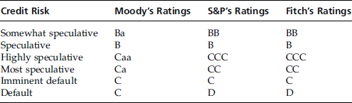
The ratings scales adopted by the three rating agencies are depicted in Tables 4.5 and 4.6.
Table 4.5 Investment Grade Ratings
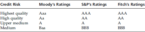
Table 4.6 Speculative Grade Ratings
As discussed, the agencies may revise their ratings during the life of the security. If a rating change is being contemplated, they will signal their intentions. S&P will place the security on credit watch. Moody's will place the security under review, and Fitch will place it on rating watch.
Bond Insurance
A company that seeks a better rating can have its issue insured in order to enhance the credit quality. In such a case, the issuer will have to pay a premium to the insurance company. But this cost will be passed on to investors in the form of a lower coupon. In the case of insured bonds, the timely payment of promised cash flows is guaranteed by the insurance company. The rating of such issues would depend on the financial health of the insurer. It would make sense to get an issue insured only by a company that enjoys a better reputation than the issuer.
Equivalence with Zero-Coupon Bonds
Consider a bond with a face value of $1,000 and two years to maturity. Assume that the coupon is 7 percent per annum payable on a semiannual basis. This bond will give rise to five cash flows per the schedule shown in Table 4.7.
Consider the first cash flow. It is like the maturity value of a zero-coupon bond with a face value of $35 that matures after six months. Similarly, the second cash flow is like the maturity value of a zero-coupon bond with a face value of $35 maturing after 12 months. The plain vanilla bond is like a portfolio of five zero-coupon bonds. This is true for any plain vanilla bond. If the bond has N coupons remaining until maturity, then it is equivalent to a portfolio of N + 1 zero-coupon bonds.
Table 4.7 Cash Flows from a Two-Year Bond
| Time Period (Months) | Cash Flow ($) |
| 6 | 35 |
| 12 | 35 |
| 18 | 35 |
| 24 | 35 |
| 24 | 1,000 |
Spot Rates
Consider the same two-year bond. It is equivalent to a portfolio of five zeros. Each zero must have its own yield to maturity. The yield to maturity of a zero-coupon bond, for a given time to maturity, is referred to as the spot rate for that period. The price of the plain vanilla bond may be expressed as
![]()
The traditional pricing equation, based on the YTM, states that
Because a plain vanilla bond is a portfolio of zeros, the correct way to price it is by discounting each cash flow at the corresponding spot rate. When we value the cash flows by discounting at the YTM, we are using an average discount rate to capture the effect of the various spot rates. The YTM of a bond is a complex average of the underlying spot rates.
The Coupon Effect
The YTM is subject to what we call a coupon effect. Consider two one-year bonds, both with a face value of $1,000. Bond A pays coupons at the rate of 7 percent per annum, whereas bond B pays a coupon at the rate of 10 percent per annum. Assume that the six-month spot rate is 6 percent per annum, while the one-year spot rate is 7.25 percent per annum.
![]()
The YTM may be calculated as
If we solve the quadratic equation, we get y = 7.2283%.
Consider bond B. The price is given by
![]()
The YTM comes out to be 7.2197 percent.
Why is it that bond A has a higher YTM than bond B? The price of one-period money is 6 percent per annum, whereas that of two-period money is 7.25 percent per annum. Two-period money is more expensive. Bond A has
![]()
of its value locked up on one-period money. Bond B, on the other hand, has
![]()
of its value locked up in one-period money. Because bond B has a greater percentage of its value locked up in one-period money, which in this case is cheaper, it is not surprising that its YTM is lower than that of bond A. The YTM, which is a complex average of spot rates, is a function of the coupon rate of a bond for a given term to maturity, which is what we term the coupon effect.
Bootstrapping
We will not have price data for zero-coupon bonds expiring exactly one period apart. In other words, we will not be in a position to compute the spot rates directly from the observable prices. Bootstrapping is a technique for obtaining spot rates from price data for plain vanilla bonds.
Table 4.8 Prices of Plain Vanilla Bonds with Varying Times to Maturity
| Term to Maturity (Months) | Price ($) |
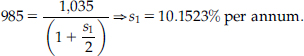
| 6 | 985 |
| 12 | 950 |
| 18 | 925 |
| 24 | 900 |
Consider the information in Table 4.8. All the bonds have a face value of $1,000 and pay a coupon of 7 percent per annum on a semiannual basis.
The one-period spot rate is given by
We know that
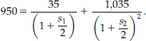
Substituting for s1, we get s2 = 12.5146 percent per annum. Similarly, using the pricing equation for the 18-month bonds and substituting for s1 and s2, we can compute s3 and, by extending the logic, find s4. This is the essence of bootstrapping.
Forward Rates
Consider a person with a two-period investment horizon. She can directly invest in a two-period zero-coupon bond or she can invest in a one-period bond and roll over her investment. The second approach is fraught with risk because we cannot predict at the outset what the one-period rate will be after one period. However, it may be possible to enter into a forward contract at the outset that locks in a rate for the one-period investment after one period. The rate implicit in such a contract is referred to as the forward rate of interest. We will denote it as ![]() . The subscript indicates that it is for a loan to be made after one period, and the superscript indicates that the loan is for one period. To rule out arbitrage, it must be the case that
. The subscript indicates that it is for a loan to be made after one period, and the superscript indicates that the loan is for one period. To rule out arbitrage, it must be the case that
![]()
If the one-period rate is 8 percent per annum while the two-period rate is 8.50 percent per annum, then
![]()
The one-period forward rate is 9.0012 percent per annum. In general, the forward-rate symbol for an m – n period loan to be made after n periods is ![]() .
.
The relationship between the n period spot rate and the m period spot rate is given by
![]()
The Yield Curve and the Term Structure
The plot of the YTM versus the time to maturity of the bond is referred to as the yield curve. On the other hand, a plot of the spot rate versus the term to maturity of the bond is called the term structure of interest rates. The term structure is also known as the zero-coupon yield curve. The two will coincide if the yield curve is flat. A flat yield curve means that all the spot rates are identical. Because the YTM is an average of spot rates, the YTM in such circumstances will be the same as the spot rate.
While plotting the yield curve or the term structure, it is important to ensure that the data being used pertain to bonds of the same risk class. In other words, if one of the bonds is AAA, then all the bonds in the data set must be AAA—that is, we should compare apples with apples and not mix up data for AAA bonds with those for T-bonds.
Shapes of the Term Structure
The term structure may take a variety of shapes. The commonly observed shapes are upward sloping or rising, downward sloping or inverted, humped, and U-shaped.
Rising yield curves will have a positive slope—that is, short-term yields will be lower than long-term yields. On the other hand, inverted yield curves are characterized by a negative slope—that is, short-term yields are higher than long-term yields. Humped yield curves tend to have lower rates at the short and long ends of the spectrum, and higher rates in between: the curve initially rises, peaks at the middle of the maturity spectrum, and then gradually slopes downward. U-shaped yield curves have the opposite shape—that is, the rates are higher at the short and long ends of the spectrum and tend to be low in between. Such curves are characterized by a curve that declines initially, reaches a trough at the middle of the maturity spectrum, and then gradually slopes upward.
Theories of the Term Structure
A variety of theories have been expounded to explain the various observed shapes of the yield curve. One popular theory is the pure or unbiased expectations hypothesis. It states that the implied forward rates computed using current spot rates are nothing but unbiased estimators of future spot rates. According to this theory, then, long-term spot rates are geometric averages of expected future short-term rates. This hypothesis can be used to explain any shape of the yield curve. Let us take an upward-sloping curve. The expectations hypothesis would explain it with the argument that the market expects spot rates to rise. If rates are expected to rise, then holders of long-term bonds will be perturbed because the prices of such bonds are expected to decline, and they are confronted with the possibility of a capital loss. Such investors will start selling long-term bonds and buying short-term bonds. This will lead to an increase in long-term yields and a decrease in short-term yields. The net result would be an upward-sloping yield curve.
Consider an inverted yield curve. This would be consistent with the view that the market expects future spot rates to fall. If so, investors will seek to sell short-term bonds and invest in long-term bonds, which will push up short-term yields and lead to declining long-run yields. The net result will be an inverted yield curve.
A humped yield curve would be consistent with the expectations that investors expect short-term rates to rise and long-term rates to fall.
The expectation of the future direction of the market is primarily a function of the expected rate of inflation. If the market expects inflationary pressures in the long run, then the yield curve will be upwardly sloping. However, if inflation rates are expected to decline in the long run, then the curve will be negatively sloped.
The Liquidity Premium Hypothesis
This hypothesis argues that the forward rate is not equal to the expected spot rate but is greater than the expectation of the future spot rate. The difference between the forward rate and the expectation of the future spot rate is termed the liquidity premium. Theory argues that because lenders generally prefer to lend short term, they must be suitably compensated if they are to be induced to lend for longer terms. This compensation takes the form of a premium for a loss of liquidity. Per this hypothesis, the yield curve should invariably be upwardly sloping, reflecting the investors' preference for liquidity. However, a declining yield curve can be explained by postulating that future spot rates may sharply decline, causing long-term rates to be lower than short-term rates, the liquidity premium not withstanding.
The Money Substitute Hypothesis
According to this theory, short-term bonds are essentially a substitute for cash. Investors generally hold only short-term bonds because of the lower perceived risk. This drives up the demand for such securities and pushes down the yield. This explains low yields at the short end of the maturity spectrum. As far as the other end is concerned, borrowers tend to issue long-term debt, which implies that they will have to access the capital market less frequently, because it minimizes the costs associated with borrowing. This leads to an excess supply at the longer end of the maturity spectrum and pushes up the yield.8
The Market-Segmentation Hypothesis
The theory postulates that the market is made up of a wide variety of investors and issuers. Each class of investors or issuers has its own requirements and tends to focus on a particular range of the maturity spectrum. The theory argues that the segments of the market are compartmentalized and there are no interrelationships between them.
The observed shape of the yield curve, in accordance with this theory, depends on the demand–supply dynamics within the market segment, and activities in a given segment have no implications for any other part of the curve. The need to constantly manage their cash leads commercial banks to primarily focus on the short end of the curve. On the other hand, institutions such as insurance companies and pension funds, whose liabilities are primarily long term, tend to focus on the long end of the market.9 There is relatively less demand for medium-dated bonds. According to this theory, yields will be relatively low at the short and long ends of the maturity spectrum and high in the middle of the term structure, which is consistent with what we call a humped yield curve.
The Preferred Habitat Theory
This theory is a slight modification of the market-segmentation hypothesis. This proposes that even though it is true that investors tend to concentrate on their chosen market segment, they can be persuaded to hold securities from other segments by offering them suitable inducements. Whereas banks generally operate at the lower end of the spectrum, an increase in yields of long-dated bonds may sometimes be adequate to persuade them to hold such securities. Similarly, an increase in short-term rates may encourage pension funds and insurance companies to invest in that segment, an area of the market they would otherwise avoid.
The Short Rate
A short rate of interest is a future spot rate of interest that may evolve over time. It is usually represented as a single period rate for the shortest period of time considered by the model on the basis of which it is postulated to evolve. In our preceding discussions, we have assumed that the shortest time period corresponds to six months.
At a given point in time, we will have a vector of spot rates corresponding to various intervals of time, and this vector can be used to derive a unique vector of current forward rates as explained earlier. However, we cannot with certainty state as to what the spot rate will be at a future point in time, because it may take on one of several values, each having an associated probability of occurrence.
At the current instant, the one-period spot rate will be equal to the one-period forward rate, which will be equal to the short rate. However, if we look at a longer time horizon, these rates will in general not be equal to each other.
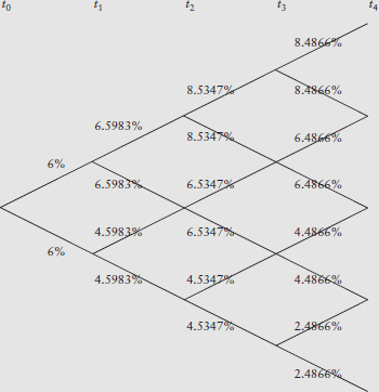
Example 4.9 illustrates the evolution of short rates over time based on the Ho and Lee model.
The tree for the evolution of short rates that we describe as follows is based on the Ho and Lee model and was originally presented in Parameswaran (2009).10 The details behind the derivation are beyond the scope of this book. The derivation assumes the term structure depicted in Table 4.9.
Table 4.9 Vector of Spot Rates
| Period | Spot Rate (%) |
| 1 | 6.00 |
| 2 | 5.80 |
| 3 | 6.05 |
| 4 | 5.90 |
In Figure 4.2, at each node there is a 50 percent probability of reaching the upper state at the end of the current period, as well as an equal probability of reaching the lower state. The current one-period spot rate is 6 percent, which is equal to the current short rate. At the end of the period, there is a 50 percent chance that the short rate will be 6.5983 percent and an equal probability that it will be 4.5983 percent. Similarly, at the end of two periods, the short rate can take on one of three possible values, whereas at the end of three periods it can take on one of four possible values.
Floating-Rate Bonds
Floating-rate notes and bonds, also referred to as floaters, are debt securities whose coupons are reset periodically based on a reference or benchmark rate. Typically, the coupon on such a security is defined as
![]()
Consider a security whose coupon is specified as
![]()
In this case, the reference rate is the yield on a five-year T-note, and the quoted margin is 75 basis points (bp). Note that the quoted margin need not always be positive. A floater may have a coupon rate specified as
![]()
In the case of a default risk-free floating-rate bond, the price of the security will always reset to par on a coupon date, although it may sell at a premium or at a discount between two coupon dates.
Consider a floater with a coupon equal to the five-year T-bond rate and assume there are two periods to maturity. The price of the bond at the end of the first coupon period will be given by
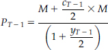
where cT − 1 is the coupon rate one period before maturity, and yT − 1 is the required yield one period before maturity. On the coupon-reset date, the YTM will be equal to the coupon because we have assumed that there is no default risk implicit in the security. Any change in the required yield, as reflected by the YTM at that point in time, will also be reflected in the coupon that is set on that day. We know that if the yield is equal to the coupon, then the bond should sell at par. Thus PT − 1 = M.
The price at the outset is given by
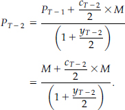
Once again, at T −2, cT − 2 = yT − 2, and PT − 2 = M. This logic can be applied to a bond with any number of coupons remaining to maturity.
Between two coupon dates, however, the price of such a floater may not be equal to par. Consider the valuation of the note at time T − 2 + k. The price is given by
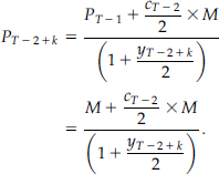
Although cT − 2 was set at time T − 2 and is equal to yT − 2, yT −2 + k is determined at time T − 2 + k and will reflect the prevailing five-year T-note yield at that point in time. In general, yT − 2 + k need not equal cT − 2 and may be higher or lower. Between two coupon dates, a floater may sell at a premium or at a discount.
Let us consider the case of floaters characterized by default risk. In this case, it is not necessary that the risk premium required by the market be constant over time. Assume that when the bond was issued the required return was equal to the five-year T-note rate +75 bp. The coupon was set equal to this rate and the bond was sold at par. 6-M hence the issue is perceived to be more risky, and the required return in the market is the five-year T-note rate +95 bp. The coupon will however be reset at the prevailing T-note rate +75 bp. This issue will not reset to par at the next coupon date.
Bonds with Embedded Options
We will consider three types of bonds with embedded options: callable, putable, and convertible bonds. All of these bonds give either the issuer or the lender an option. As we have seen, an option gives the holder the right to take a course of action. Because no one will give a right away for free, the holder has to pay a price or a premium to the seller of the option. In the case of bonds with embedded options, if the option is with the issuer, then he must pay for it, and the price of the bond will be less than that of a plain vanilla bond. However, if the option were to be with the lender, then it will manifest itself as a higher price compared to that of a plain vanilla bond.
Callable Bonds
Such bonds contain a call option; that is, they give the issuer the right to call away the bond from the lender before maturity. The issuers can in the case of such bonds change the maturity of the bonds by prematurely recalling them. When will such a bond be recalled? When market interest rates are declining. Under such circumstances, the issuer can recall the existing bonds and replace them with a fresh issue that can be issued with a lower coupon because of the changed circumstances.
The call provision works against the lender because she may have to part with the bond when the market rates are falling, which is precisely a situation in which she will desire to hold on to the bonds and keep earning a high coupon. To compensate for this, she will demand a higher yield as compared to what she would from a plain vanilla bond of the same credit quality. This will manifest itself as a lower price. Whether we view it from the issuer's perspective or the lender's, a callable bond must sell at a lower price compared to an otherwise similar plain vanilla bond.
Such bonds may be discretely callable or continuously callable. A discretely callable bond may be recalled only at certain prespecified dates—for instance, at the coupon dates over a portion of the bond's life. A continuously callable bond may be called at any time after it becomes callable.
As we have just mentioned, a bond may be recalled only when it becomes callable. This implies that it may not be callable right from the outset. Issuers generally specify a call-protection period, which is a period of time during which the bond may not be recalled regardless of what happens to the market rate of interest. A discretely callable bond can usually be recalled on any coupon payment date after the call-protection period ends, whereas a continuously callable bond may be recalled at any time from the end of the call-protection period until the maturity date of the bond. Bonds with a call-protection period are referred to as deferred callable bonds, and they serve to provide holders with relatively greater certainty.
The price at which the bond can be recalled is referred to as the call price. In many cases, a bond may be recalled at par by an issuer. At times, however, the issuer may specify a call premium—that is, he will pay a value higher than the face value of the bonds if and when the issue is recalled. The call premium is usually set equal to one year's coupon.
Holders of callable bonds are extremely vulnerable to reinvestment risk. First, it is increasingly likely that they will experience a return of cash in a falling interest-rate environment, in a falling interest-rate environment, which means they will have to face the specter of reinvesting their corpus at a lower rate of interest. Second, the potential for price appreciation in a falling rate environment is relatively limited as compared to a plain vanilla bond. Why do bond prices increase in value? Because yields are declining in the market. But in the case of callable bonds, this is precisely the situation in which the bond can be recalled, which means the buyer of such bonds in a falling interest-rate environment is constantly exposed to the risk of having to part with it at the call price. This aspect is referred to as price compression.
Yield to Call
In the case of callable bonds, it is a normal practice to compute the yield to call (YTC). For a given call date, all the cash flows from the current point in time until the call date are specified, and the discount rate that makes the present value of these cash flows equal to the dirty price of the bond is computed. The cash flows will be the coupons scheduled to be paid on or before the call date and the call price. The price at which the bond is recalled may in certain cases vary with the call date—that is, the call price may be a function of the call date.
The formula for the YTC, assuming that the bond is callable after N* coupons have been paid, may be stated as

This looks similar to the pricing equation that corresponds to the YTM calculation. But there are two key differences. First, M*, which is the call price, need not equal the face value. Second, N*, the number of coupons until the call dates, will be ≤ N.
Example 4.10 illustrates the computation of the yield to call for a callable bond.
Consider a bond with 20 years to maturity and a face value of $1,000. Assume that the coupon rate is 7 percent per annum and that the current price is $925. The first call date is eight years away; if the bond is called, the issuer will pay one year's coupon as the call premium. The YTC can be computed from the following equation:
The solution comes out to be 8.9503 percent.
Putable Bonds
In the case of a putable bond, the holders have a put option: they can prematurely return the bond to the issuer and claim the face value. Such an option will be exercised when the market interest rates have risen. Under such circumstances, the holders can return the old bonds, which are yielding a relatively lower coupon, and use the proceeds to buy bonds yielding a higher coupon. Because the option in these cases is with the holders, they have to pay for it. This will manifest itself as a higher price as compared to that for a plain vanilla bond carrying the same coupon. A putable bond will sell for a lower yield as compared to a plain vanilla bond.
Consider the relative coupons for plain vanilla, callable, and putable bonds for a given risk class. The callable will have to offer the highest coupon, whereas the putable can be issued with the lowest coupon. After the issue, if we were to compare bonds with and without call and put options for a given coupon rate, the callable will have the lowest price or the highest yield, and the putable will have the highest price or the lowest yield.
The yield to put is typically defined as the discount rate that makes the present value of the cash flows from the bond equal to its price, assuming that the bond is held to the first put date.
Convertible Bonds
Convertible bonds allow holders to convert the debt securities into shares of stock of the issuer. The number of shares that an investor will receive if he not we. were to convert the bond is known as the conversion ratio. Consider a bond with a face value of $1,000 that can be converted to 50 shares of stock. The conversion ratio is 50. The conversion price is the face value divided by the conversion ratio—in this case, $20. The conversion value is the value of the shares if the bond were to be converted immediately. If we assume that the current share price is $22.50, then the conversion value is $1,125.
The minimum value of a convertible is the greater of the conversion value and the value that will be obtained if the bond were to be valued under the assumption that it is a plain vanilla bond. The latter value is termed the straight value of the bond.
The computation of the conversion and straight values for a convertible bond is illustrated in Example 4.11.
Consider a convertible bond with a face value of $1,000 and five years to maturity. Assume that the coupon is 7 percent per annum payable on a semiannual basis, and that the conversion ratio is 50.
If the current stock price is $21, then the conversion value is $1,050. If we assume that the YTM of a plain vanilla bond with the same risk is 8 percent per annum, then the straight value will be $959.45. Because 1,050 is greater than 959.45, the price of the convertible must be ≥ $1,050.
But what if the YTM of a comparable bond were to be 5 percent? The straight value will be $1,087.52. In this case, the value of the convertible must be ≥ $1,087.52.
Using Short Rates to Value Bonds
Let us consider a segment of the interest-rate evolution tree (Figure 4.3) that we referred to earlier.
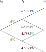
Figure 4.3 A Segment of the Short-Rate Tree
A Segment of the Short-Rate Tree
Consider a plain vanilla bond maturing at t2, with a face value of $100, paying a coupon of 6 percent per annum on a semiannual basis. At time t2, there are three possible nodes. At each node, the payoff will be $103.
The value of the bond at the upper node at t1 is
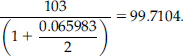
Similarly, the value at the lower node at t1 is
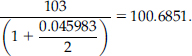
Because, given a node, the probability on an up move is equal to that of a down move, which in turn is equal to 50 percent, we can compute the value of the bond at t0 as
![]()
Consider a callable bond, which we will assume can be called back at the face value.11 Because the value at the upper node at t1 is less than the call price, the bond will not be recalled. However, at the lower node the value is higher than the call price and the issuer would like to exercise his call option. The price of the callable bond at t0 may be computed as
![]()
As can be seen, the presence of the call option leads to a reduction in the bond value. Assume a bond with a put option. The holder will exercise it only if the value of the bond is less than its face value, assuming that he has the right to put it back at the face value. If so, the value at t0 is given by
![]()
For obvious reasons, the put option makes the bond more valuable.
Price Volatility
It is common knowledge that long-term bonds are more price sensitive to a change in yield than comparable short-term bonds. This can be easily explained. The present value of a cash flow is given by ![]() .
.
The further away the cash flow—that is, the larger the value of t—the greater will be the impact of a change in the discount rate. Because long-term bonds have more cash flows coming at distant points in time, it can be concluded that their prices were more volatile. However, a second fact was subsequently noticed. For a given term to maturity, a zero-coupon bond was more price sensitive than any coupon-paying bond with the same term to maturity. This was perplexing because the bonds have the same term to maturity.
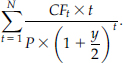
Frederick Macaulay came up with the concept of duration to explain this phenomenon. The crux of the idea is the following. A plain vanilla bond, as we have seen earlier, is a portfolio of zero-coupon bonds. Each component zero will have its own term to maturity. When we state that a plain vanilla bond has a term to maturity of T years, we are taking cognizance of the term to maturity of only the last of the component zeros. Macaulay argued that the effective term to maturity of a plain vanilla bond ought to be a weighted average of the terms to maturity of each component zero. The weight attached to a cash flow, he postulated, should be the present value of the cash flow divided by the price of the bond. Because the price of a bond is the sum of the present values of all the cash flows received from it, the weights defined by Macaulay will add up to 1. The Macaulay duration of a bond may be defined as
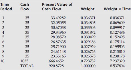
Example 4.12 demonstrates the computation of the duration for a plain vanilla bond.
Consider a bond with a term to maturity of five years and a face value of $1,000. Assume that the coupon is 7 percent per annum and that the YTM is 9 percent per annum. The computation of the duration is shown in Table 4.10.
The price of the bond is $920.8728. The weighted average term to maturity, which we term as the duration of the bond, is 8.537804 semiannual periods, or 4.26892 years. Although the bond has a stated term to maturity of five years, its effective term to maturity is only 4.26892 years. It should be obvious why a five-year zero-coupon bond will be more price sensitive: because in the case of the zero, with a single cash flow, there is no difference between its stated term to maturity and its effective term to maturity. Irrespective of the value of T, a T-year zero will always have a higher duration than a T-year plain vanilla bond and will therefore be more price sensitive.
Table 4.10 Computation of Duration
A Concise Formula
For a plain vanilla bond, we can derive a concise expression for the duration. Let us first redefine a few variables.
![]()
It can be shown that the duration of a bond is given by
![]()
Using the data that we considered for the preceding illustration,
![]()
Duration and Price Volatility
The rate of change of the percentage change in price with respect to yield is a function of the duration of the bond. The relationship may be expressed as
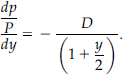
In this expression, D is the duration of the bond expressed in years.
The expression  is referred to as the modified duration of the bond, Dm.
We know that for a finite price change, the percentage change in price is ![]() . In the limit we can express it as dP/P. The rate of change of the percentage change in the price with respect to the yield is equal to the modified duration of the bond. It is duration, and not the term to maturity, that is an accurate measure of interest-rate sensitivity.
. In the limit we can express it as dP/P. The rate of change of the percentage change in the price with respect to the yield is equal to the modified duration of the bond. It is duration, and not the term to maturity, that is an accurate measure of interest-rate sensitivity.
We must point out that the duration of a bond technically should be perceived as a measure of interest-rate sensitivity. It cannot always be perceived as a measure of the effective average life of the bond.
Properties of Duration12
- The duration of a bond increases with its term to maturity. There are two reasons for this. First, the principal repayment is a major component of the bond's present value and has a significant impact on its duration. As the time to maturity is increased, the repayment of principal is postponed, which serves to increase the duration. Second, as compared to a short-term bond, a long-maturity bond has cash flows arising at later points in time, which serves to increase the duration.
- The duration of a bond is inversely related to its coupon rate. There are two reasons for this. First, high coupon bonds have greater amounts of cash flow occurring before the maturity date. This serves to reduce the relative impact of the principal repayment on duration. Second, the impact of discounting is less on the earlier cash flows as compared to greater cash flows. The greater the coupon, the more the relative present value of the earlier cash flows, which serves to reduce the duration of the security.
- Duration is inversely related to the YTM of the bond. Duration is computed by weighting the times to maturity of each coupon payment by its contribution to the present value of the bond. The higher the discount rate, the lower the present value of a cash flow. However, increasing the discount rate has a greater impact on long-term cash flows as compared to shorter-term cash flows. The relative weightage of shorter term cash flows is increased as we increase the YTM, which serves to bring down the duration of the bond.
Dollar Duration
The dollar duration of a bond is defined as the product of the modified duration of the bond and its price. In the preceding illustration, the price of the bond was $920.8728, and its modified duration was 4.0851 years. The dollar duration is 920.8728 × 4.0851 = 3,761.8574.
Convexity
The price–yield relationship for a plain vanilla bond is convex in nature. Duration is a measure of the first derivative and varies along with yield. To factor in the convex nature or curvature of the bond, we need to compute the second derivative.
Figure 4.4 illustrates the price–yield relationship for a plain vanilla bond. The bond was assumed to have 10 years to maturity, a face value of $1,000, and a coupon of 7 percent per annum payable semiannually.
From the Taylor series expansion, we can state that
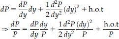
where h.o.t. stands for higher-order terms.
The first term on the right-hand side captures the duration effect. The second expression is the convexity effect. The convexity of a bond is defined as ![]() . The percentage price change because of the convexity effect is
. The percentage price change because of the convexity effect is
The convexity can be computed as 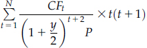 .
.
The calculation of the convexity for the five-year bond with a coupon of 7 percent is depicted in Table 4.11.
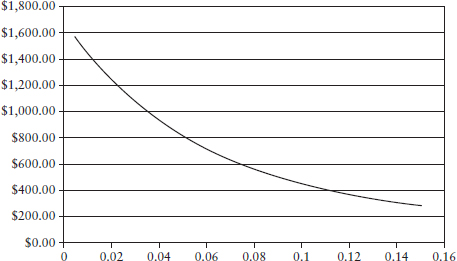
Figure 4.4 The Price Yield Relationship
Table 4.11 Computation of Convexity
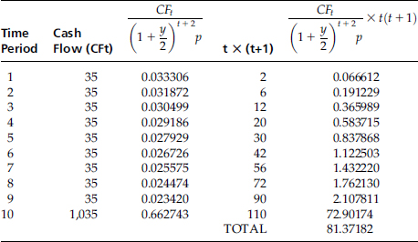
The convexity in half years is 81.37182. The convexity in annual terms can be obtained by dividing this number by 4.13 In this case, the annual convexity is 20.3430.
Consider a finite change of 100 bp in the annual YTM. The price at a YTM of 10 percent is $884.1740. The percentage price change is
![]()
The percentage price change as captured by duration is −Dm × dy. The modified duration of the bond is
![]()
The price change as captured by duration is −4.0851 × 0.01 = −0.040851 ≡ −4.0851%.
The price change because of the convexity effect is 0.5 × 20.3430 × (0.01)2 = 0.001017 ≡ 0.1017%
The percentage price change as captured by both the factors combined is −4.0851% + 0.1017% = −3.9834%. The result is fairly close to the exact percentage price change, and a combination of duration and convexity does a better job than duration alone.
A Concise Formula
There is a closed-form expression for computing the convexity of a plain vanilla bond. It may be stated as
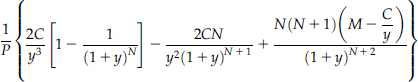
where, as before, C ≡ periodic (in our case, semiannual), coupon y ≡ semiannual YTM, and N ≡ number of coupons remaining until maturity.
In our illustration, C = $35, y = 0.045, N = 10, and P = $920.8728. Substituting for the variables, we get convexity = 81.3718.
Dollar Convexity
The dollar convexity of a bond is equal to its convexity multiplied by its price. In our illustration, the price is 920.8728 and the convexity is 20.3430. The dollar convexity is 18,733.3150.
Properties of Convexity
The following properties are valid for the convexity of plain vanilla bonds:14
- As the YTM increases, the convexity decreases and vice versa. This property of option-free bonds is referred to as positive convexity.
- For a given value of the YTM and time to maturity, the lower the coupon, the greater the convexity of the bond. For a given yield and time to maturity, a zero-coupon bond will have the highest convexity.
- For a given value of the YTM, and modified duration, the lower the coupon, the lower the convexity of the bond. For a given yield and modified duration, a zero-coupon bond will have the lowest convexity.
Immunization
Consider the case of a pension fund that promises to pay a return of 4.9688 percent per annum compounded semiannually on an initial investment of $100,000 after eight years. If it were to invest the corpus in a bond, it is exposed to two types of risks. The first is reinvestment risk, or the risk that the cash flows received at intermediate stages may have to be invested at lower rates of interest. The second, termed price or market risk, is the risk that interest rates could increase, causing the price of the bond to fall at the end of the investment horizon. The two risks work in opposite directions. The issue, therefore, is whether there is a bond that will ensure that the terminal cash flow is equal to the amount required to satisfy the liability, irrespective of whether rates rise or fall. The process of protecting a bond portfolio against a change in the interest rate is termed immunization.
We are considering a simple immunization strategy in which we have to immunize a portfolio required to satisfy a single liability. We need to satisfy two conditions in such cases. First, the present value of the liability should be equal to the amount invested in the bond at the outset. Second, the duration of the bond should be equal to the investment horizon.
Consider a bond with a face value of $1,000 and 10 years to maturity. Assume that the coupon rate is equal to the YTM and equal to 4.9688 percent per annum. It can be shown that the duration is eight years.
Assume a one-time change in interest rates right at the outset. Assume that the interest rate increases from 4.9688 percent per annum to 5.50 percent per annum. The terminal value of the coupons from the bond at the end of eight years is given by
If the YTM for two-year bonds after eight years is 5.50 percent per annum, the price at which 100 bonds can be sold is 100 × 990.0681 = $99,006.8080. The total terminal cash flow is $148,108.4386. Table 4.12 gives the terminal cash flow for various values of the interest rate.
Analysis
The income from reinvested coupons steadily increases with the interest rate, whereas the price of the bond at the time of sale steadily decreases with the interest rate. When there is no change in the rate, the terminal cash flow from the bond is exactly adequate to meet the liability. In all other cases, there is a surplus. Under all circumstances, the terminal cash flow from the bond is adequate to meet the liability. If the pension fund were to invest in an asset, whose duration is equal to the time to maturity of its liability, then the funds received will always be adequate to meet the contractual outflow. To meet this requirement, four conditions must be satisfied. First, the amount invested in the bonds must be equal to the present value of the liability. In this case, because the bond is assumed to be selling at par, we need to invest in 100 bonds. Second, the duration of the asset must equal the maturity horizon of the liability. Third, there must be a one-time change in the interest rate right at the very outset. Fourth, there must be a parallel shift in the yield curve.
Treasury Auctions
The Treasury issues T-bills, T-notes, and T-bonds by way of auctions. The auction procedure is described in detail in the next chapter on money market securities. In Examples 4.13 and 4.14 we will illustrate two recent auctions of notes and bonds to describe the salient features.
Example 4.13 (Issue of a Five-Year T-Note)
Consider the following details:
- Interest rate = 2.5000 percent
- High yield = 2.6050 percent
- Price = $99.510730
- Accrued interest = None
- Issue date = March 31, 2010
- Maturity date = March 31, 2015
- Original issue date = March 31, 2010
- Dated date = March 31, 2010.
This is an issue of a brand-new security with a maturity of five years. The issue date is the same as the original issue date: March 31, 2010. The maturity date is five years after the issue date because the security has a life span of five years. The dated date is the first date from which coupons begin to accrue; in this case, it is the same as the issue date.
The auction cleared at a YTM of 2.605 percent; that is, the quotes were arranged in ascending order of bids (yields), and the highest bid at which some securities were awarded was 2.605 percent. The coupon was unknown at the outset because this was a new issue. The Treasury will set the coupon after rounding down the market yield to the nearest multiple of 0.125, which in this case is 2.5 percent. The issue price may be determined as follows:
![]()
Table 4.12 An Immunized Portfolio
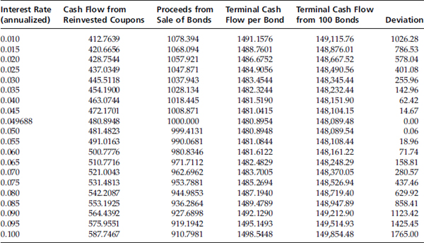
Example 4.14 (Reopening of a 30-Year T-Bond)
Consider the following details.
- Interest rate = 4.6250
- percent High yield = 4.7700 percent
- Price = $97.692939
- Accrued interest = 7.53798
- Issue date = April 15, 2010
- Maturity date = February 15, 2040
- Original issue date = February 16, 2010
- Dated date = February 15, 2010.
This is a reopening of an existing treasury security. In other words, on February 16, 30-year T-bonds were issued, and on April 15 a fresh issue was made of 29-year, 10-month bonds with the same coupon; that is, the auction added to the supply of securities that were already available in the market. This is the import of the word reopening.
The issue date is two months after the original issue date. February 15 was a market holiday. Although the dated date is February 15, the original issue date is February 16.
The auction cleared at 4.77 percent. The coupon was known from the outset, because the security was already in existence. The accrued interest and price may be computed as follows. The number of days from the dated date until the issue date is 59. The total number of days in the coupon period is 181. The accrued interest per $1,000 of face value is given by
![]()
The clean price may be determined as follows. The fractional period until the next coupon is 122/181 = 0.6740. The dirty price is given by

The clean price is = $98.4467 − $0.7538 = $97.6929.
Frequency of Issue
Various Treasury notes—2, 3, 5, and 7 years—are auctioned on a monthly basis. Ten-year T-notes are auctioned on a quarterly basis in February, May, August, and November. Reopenings take place in March, April, June, July, September, October, and December. Issues are reopened one month after original issuance and, once again, two months after original issuance.
Thirty-year T-bonds are auctioned in February, May, August, and November. The reopening schedule is identical to that for 10-year T-notes.
When Issued Trading
The when issued (WI) market is a market for forward trading of a bond whose issue has been announced but has not yet taken place. Trades in this market take place from the date of announcement of a forthcoming auction of government securities until the actual issue date of the securities. The WI market helps potential bidders to gauge the market's interest in the security before the actual auction. This will have ramifications for the bidding strategies of market participants and will have a bearing on the outcome of the auction.
Traders can take both long and short positions in the WI market, with settlement being scheduled for the issue date. Trades in this market represent forward contracts, with the issue date being the settlement date. On and before the date of the auction, the issues trade on a yield basis. The actual price in dollars can be established only after the Treasury sets the coupon. A five-year T-note is quoting in the WI market at 5 percent. If the coupon is set at 4.875, then the price of the security will be 99.4530. However, if the coupon is set at 5.125, the price will be 100.547. Starting with the day after the auction, securities in the WI market are quoted on a price basis because the coupon has already been established.
Price Quotes
Bond prices are always quoted per $100 of face value. The reason is the following. Consider two bonds, one with a face value of $1,000 and another with a par value of $2,000. Assume that both securities are quoting at $1,500. The first is a premium bond and the second a discount bond. However, this cannot be discerned from the observed price unless the corresponding face value is also specified. On the other hand, if the price were to be expressed for a par value of $100, then any value less than 100 would signify a discount bond whereas a value more than 100 would connote a premium bond.
In the United States, market prices are quoted as a percentage of par plus thirty-seconds. Consider a quote of 97-08. This does not mean a price of $97 and 8 cents per $100 of face value. What it means is that the price per $100 of face value is 97 + 8/32 or $97.25. So, if we were to buy bonds with a face value of $1 million, the amount payable will be 1,000,000 × 97.25/100 = $972,500.
The quoted prices are always clean prices. To compute the exact amount payable by the buyer, the accrued interest has to be calculated per the prescribed convention and added to the clean price.
Bond Futures
Futures contracts are available on 2-, 5-, and 10-year T-notes and on 30-year T-bonds. The underlying asset for the 2-year note contract is a T-note with a face value of $200,000. Multiple grades are allowable for delivery with the stipulation that the deliverable grade must have an original maturity of not more than 5 years and 3 months, an actual maturity of not less than 1 year and 9 months from the first day of the delivery month, and not more than 2 years from the last day of the delivery month. At any point in time, 5 contract months from the March quarterly cycle are listed. The last trading day is the last business day of the calendar month.
The underlying asset for the 5-year note contract is a T-note with a face value of $100,000. Multiple grades are allowable for delivery with the stipulation that the deliverable grade must have an original maturity of not more than 5 years and 3 months and an actual maturity of not less than 4 years and 2 months from the first day of the delivery month. At any point in time, 5 contract months from the March quarterly cycle are listed. The last trading day is the last business day of the calendar month.
The underlying asset for the 10-year note contract is a T-note with a face value of $100,000. Multiple grades are allowable for delivery with the stipulation that the deliverable grade must have an actual maturity of not less than 6 years and 6 months from the first day of the delivery month and not more than 10 years from that date. At any point in time, 5 contract months from the March quarterly cycle are listed. The last trading day is the seventh business day preceding the last business day of the calendar month.
The underlying asset for the 30-year bond contract is a T-bond with a face value of $100,000. Multiple grades are allowable for delivery with the stipulation that the deliverable grade must, if it is callable, not be callable for at least 15 years from the first day of the delivery month. Noncallable bonds must have a maturity of at least 15 years from the first day of the delivery month. At any point in time, 5 contract months from the March quarterly cycle are listed. The last trading day is the seventh business day preceding the last business day of the calendar month. All note and bond futures contracts are delivery settled.
STRIPS
STRIPS is an acronym for separate trading of registered interest and principal of securities. As the name suggests, these represent zero-coupon debt securities created by separately selling the entitlement to each cash flow from the mother security. As we saw earlier, a conventional bond is nothing but a portfolio of zero-coupon bonds. A 10-year T-note can be stripped into 21 zero-coupon securities, where the first 20 represent the respective coupon payments and the last represents the face value. The U.S. Treasury does not strip eligible securities. However, a trader who holds a Treasury note or bond can seek to have the issue converted into the coupon and principal components. The request can be made at any point in time before the maturity date of the security. Once stripped, each zero-coupon component can be traded separately. Each component will have a unique CUSIP number.15 All interest-based strips that mature on the same day are assigned a common CUSIP number, regardless of the mother bond from which they are created. However, principal strips that mature on a given day are assigned different CUSIP numbers.
A Treasury note or a bond can be not only stripped but also reconstituted; that is, a trader who holds the entire set of component zeros can have the original or parent Treasury security regenerated.
Why is the STRIPS program popular? As we have seen, immunization strategies require the matching of the duration of the assets of the institution with that of its liabilities. Unlike coupon-paying bonds, which have constantly changing durations, zero-coupon bonds always have a duration equal to their remaining term to maturity. Zeros are invaluable for implementing such a strategy. Besides, whereas a 30-year note will have a duration that is substantially less than 30 years, by stripping it into 61 component securities, we can create zeros with durations ranging from 6 months to 30 years.16
Endnotes
1. The same can be explained by demonstrating that the partial derivative of the price with respect to the yield is negative. This is shown in the appendix.
2. Remember we are using the actual–actual day-count convention.
3. Even if the bond were to mature after a year, there will be a capital gain or a loss.
5. As explained earlier, we are pricing the bond based on 20 half years to maturity and not on 10 years.
6. On an ex post basis, we will know the selling price.
7. Notice that we have taken the coupons only for the first 16 periods.
10. Sunil Parameswaran, Futures and Options: Concepts and Applications (New Delhi: McGraw-Hill, 2010).
11. In other words, there is no call premium.
13. In general, we have to divide by the square of the frequency of compounding.
15. CUSIP is the acronym for Committee on Uniform Securities Identification Procedures.