
CHAPTER 9
Mortgages and Mortgage-Backed Securities
Introduction
In most developed countries, the right to own a home is largely considered a fundamental right. However, few people are in a position to pay the cost of buying a home from their own personal funds, so most of the money required to buy a home must be borrowed. A loan that is collateralized by real estate property is called a mortgage loan. The lender is called the mortgagee, and the borrower is called the mortgagor. In the event that the mortgagor defaults on the loan, the lender can seize the property and sell it to recover what is due him. This is called the right of foreclosure.
Market Participants
There are three categories of players in the mortgage market: (1) mortgage originators; (2) mortgage servicers; and (3) mortgage insurers.
Mortgage Originator
Who is a mortgage originator? The original lender or the party who first extends a loan to the acquirer of the property is called the mortgage originator. Originators include:
- Thrifts or savings-and-loan associations;
- Commercial banks;
- Mortgage bankers;
- Life insurance companies; and
- Pension funds.
Income for the Originator
The originator gets income from various sources. First, when a loan is granted, the originator will levy an origination fee. The fee is expressed in terms of points, with each point representing 1 percent of the borrowed funds. For example, if a lender charges 1.5 points on a loan of $200,000, the origination fee will amount to $3,000. Most originators will also levy an application fee and certain processing fees.
The second source of income is the profit that can be earned if and when the mortgage loan is sold by the originator to another party. A mortgage loan is a type of debt, so it is vulnerable to interest-rate fluctuations. If the interest rate declines, such a sale leads to a gain for the originator. This is called a secondary marketing profit. Of course, if interest rates rise after the loan is disbursed, the originator will incur a loss when the loan is sold.
If the originator decides to hold the loan as an asset rather than sell it, periodic income will be earned in the form of interest.
Mortgage Servicers
Every mortgage loan must be serviced. Mortgage loan servicing includes the following:
- Collecting monthly payments and forwarding the proceeds to the owner of the loan;
- Sending payment notices to mortgagors;
- Reminding mortgagors whose payments are overdue;
- Maintaining records of principal balances;
- Administering escrow balances for real estate taxes and insurance purposes;
- Initiating foreclosure proceedings if necessary; and
- Furnishing tax information to mortgagors when applicable.
Mortgage servicers include bank-related entities, thrift-related entities, and mortgage bankers.
Escrow Accounts
An escrow account is a trust account held in the name of the home owner to pay statutory levies such as property taxes, as well as insurance premiums. The maintenance of such an account helps to ensure that payments are made when due, because it becomes the lender's responsibility to do so.
In most cases, the borrower makes deposits on a monthly basis, along with the loan payment, and the payments accrue at the lender. The amount required to be deposited every month is a function of the cost of insurance and the tax assessment of the property concerned. It fluctuates from year to year.
Income for the Servicer
The primary source of income is the servicing fee, which is a fixed percentage of the outstanding mortgage balance. Because the mortgage loan is an amortized loan, where the outstanding principal declines with each payment, the revenue from servicing, in dollar terms, will decline over time. The second source of income arises on account of the interest that can be earned by the servicer from the escrow account that the borrower often maintains with the servicer. The third source of revenue is the float earned on the monthly mortgage payment. This opportunity arises because there is a delay that is permitted between the time the servicer receives the monthly payment and the time that the payment has to be sent to the investor.
Mortgage Insurers
There are two types of mortgage-related insurance. The first type, mortgage insurance or private mortgage insurance, is originated by the lender to insure against default by the borrower. It is usually required by lenders on loans with a loan-to-value (LTV) ratio that is greater than 80 percent. The amount insured will be some percentage of the loan, and it may decline as the LTV declines.
What is the LTV ratio? Every borrower will have to make a down payment, which is the difference between the price of the property and the loan amount. The LTV ratio is obtained by dividing the loan amount by the market value of the property. The lower the LTV ratio, the greater the protection for the lender in the event of default by the borrower.
The second type of mortgage-related insurance—typically called credit life—is acquired by the borrower, usually through a life insurance company. This is not required by the lender. Such policies provide for the continuation of mortgage payments after the death of the insured person so that survivors can continue to live in the house.
Government Insurance and Private Mortgage Insurance
As we have seen, lenders insist on insurance if the LTV ratio is more than 80 percent. However, low- to middle-income borrowers may not be in a position to deposit 20 percent of the value of the property. At the same time, their credit rating makes them ineligible to obtain insurance from private parties. To facilitate the acquisition of properties by this strata of society, government agencies are available that provide loan guarantees in lieu of insurance. These agencies include:
- The Federal Housing Administration (FHA);
- The Department of Veterans' Affairs (VA); and
- The Department of Agriculture's Rural Housing Service (RHS).
Borrowers who are not eligible for loans from these agencies must obtain private mortgage insurance (PMI).
Secondary Sales
Once a loan is granted, the originator can either hold it as an asset or sell it to an investor who may hold it as an investment or pool it with many other individual mortgage loans and use them as collateral for the issuance of securities. Of course, the issuance of securities backed by a pool of underlying mortgages may be undertaken by the originator. When a mortgage pool is used as collateral for the issuance of a security, it is said to be securitized.
Two federally sponsored credit agencies and many private agencies buy mortgages, pool them, and issue securities backed by the pool to investors. Such agencies are referred to as conduits. The two federally sponsored agencies are the Federal National Mortgage Association (Fannie Mae) and the Federal Home Loan Mortgage Corporation (Freddie Mac). Such agencies buy what they call a conforming mortgage, or one that meets the underwriting criteria established by the agencies from the standpoint of being eligible to be included in a pool for the purpose of being securitized. A conforming mortgage must satisfy three criteria: (1) PTI ratio, (2) maximum LTV ratio, and (3) maximum loan amount.
The payment-to-income (PTI) ratio is the ratio of monthly payments (the loan payment plus any real estate tax payments) to the borrower's monthly income. The lower the ratio, the greater is the likelihood of the borrower being able to pay as scheduled.1
Mortgages that are nonconforming because they are for amounts in excess of the purchasing limit set by these agencies are termed jumbo mortgages. Those that do not meet the underwriting guidelines such as credit quality or LTV ratio are termed subprime mortgages.
Risks in Mortgage Lending
Investors who invest in mortgage loans are exposed to four main risks: (1) default risk; (2) liquidity risk; (3) interest-rate risk; and (4) prepayment risk.
Default Risk
Default or credit risk is the risk that the borrower will default. For government-insured mortgages, the risk is minimal because the insuring agencies are government sponsored. For privately insured mortgages, the risk can be gauged by the credit rating of the insurance company. For uninsured mortgages, the risk will depend on the credit quality of the borrower.
Liquidity Risk
Mortgage loans tend to be rather illiquid because they are large and indivisible. Although an active secondary market exists for such loans, bid–ask spreads are large relative to other debt instruments.
Interest-Rate Risk
The price of a mortgage loan in the secondary market moves inversely with interest rates, just like any other debt security. Moreover, because the loans are for long terms to maturity, the impact of an interest-rate change on the price of the mortgage can be significant.
Prepayment Risk
Most home owners pay off all or a part of their mortgage balance before the maturity date. Payments made in excess of the scheduled principal repayments are called prepayments. Prepayments occur for one of several reasons. First, borrowers tend to prepay the entire mortgage when they sell their home. The sale of the house may be the result of a change of employment that necessitates moving, the purchase of a more expensive home, or a divorce in which the settlement requires sale of the marital residence.
Second, if market interest rates decline below the loan rate, the borrower may prepay the loan because of the ability to refinance at a lower rate. Third, in the case of home owners who cannot meet their mortgage obligations, the property will be repossessed and sold. The proceeds from the sale will be used to pay off the mortgage in the case of uninsured mortgages. For an insured mortgage, the insurance company will pay off the balance. Finally, if the property is destroyed by a so-called act of God, the insurance proceeds will be used to pay off the mortgage. The effect of prepayments, regardless of the reason, is that the cash flows from the mortgage become unpredictable.
Example 9.1 presents a detailed illustration of the refinancing of a mortgage loan.
Cindy Hopkins has taken a mortgage loan for $800,000. It is a 10-year mortgage with a nominal interest rate of 12 percent per annum. Installments are due every 6 months, and interest is compounded semiannually.
At the end of the first year, just after she has paid the second installment, the interest on housing loans drops to 10.8 percent per annum. The refinancing fee is 1.75 percent of the amount being refinanced. If Cindy's opportunity cost of funds is 9.6 percent per annum, is refinancing an attractive option?
The quantum of the semiannual interest payment is given by
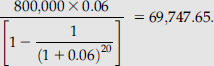
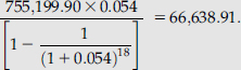
From the discussion of amortized loans in Chapter 2, we know that the amount outstanding after the second installment is
![]()
The cost of refinancing is
![]()
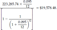
The installment amount if the loan is refinanced is
So the saving every 6 months for 18 periods is
![]()
The present value of the saving is
![]()
The net saving is
![]()
Because the net saving is positive, refinancing is an attractive proposition.
Other Mortgage Structures
The level-payment mortgage, which entails a constant monthly payment for the life of the mortgage, is the simplest of mortgage structures. Other mortgage loans with more complex features are possible. We will discuss some of them.
Adjustable-Rate Mortgage
In an adjustable-rate mortgage (ARM), the interest rate is not fixed for the life of the loan but is reset periodically. The monthly payments will rise if the interest rate at the time of resetting is higher than previously, and it will fall if the interest rate declines. The rate on such mortgages is linked to a benchmark such as the LIBOR or the rate on Treasury securities. Example 9.2 illustrates such a mortgage loan, assuming that rates are reset at the end of every year.
Consider a four-year loan with an initial principal of $800,000. Payments are to be made monthly, with the interest rate being reset every year. Assume that the benchmark is LIBOR and that the mortgage rate is LIBOR + 150 basis points (bp). Assume that the values of LIBOR observed over the next three years are as shown in Table 9.1.
Table 9.1 Observed Values for LIBOR
| Time in Years | LIBOR |
| 0 | 4.20 |
| 1 | 4.56 |
| 2 | 4.14 |
| 3 | 4.74 |
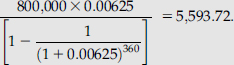
The monthly installment for the first year is
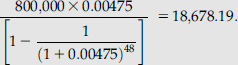
The outstanding balance at the end of the first year is
![]()
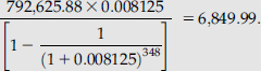
The monthly installment for the second year is
The outstanding balance at the end of the second year is
![]()
The monthly installment for the third year is
The outstanding balance at the end of the third year is
![]()
The monthly installment for the fourth year is
The outstanding balance at the end of the fourth year is zero.
Option to Change the Maturity
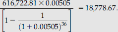
In the case of certain ARMs, the borrower may be given the option to keep the monthly installment at the initial level and have the maturity date altered every time the rate is reset. Let us see the implications of this for the mortgage discussed in the preceding example.
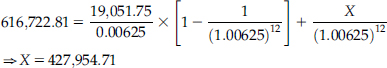
The outstanding balance after one year is $616,722.81. If we keep the equated monthly payment at $18,678.19, the life of the loan if the rate is reset at 9 percent is given by
![]()
Rate Caps
In the case of ARMs, there may be a cap on how much the interest rate may increase or decrease per period. The cap may be a periodic cap or a lifetime cap. Consider a four-year mortgage with a principal of $800,000. Assume that payments are made monthly and that the interest rate every period is the prevailing LIBOR at the start of the period plus 150 bp. The values of LIBOR observed over the next three years are as shown in Table 9.2.
Assume that there is a periodic cap of 1.5 percent and a lifetime cap of 9 percent. If so, the applicable mortgage rates for each period would be as shown in Table 9.3.
Table 9.2 Observed Values for LIBOR
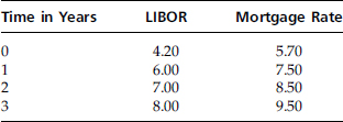
Table 9.3 Mortgage Rates in the Presence of a Cap
| Period | Mortgage Rate |
| 0 | 5.70 |
| 1 | 7.20 |
| 2 | 8.50 |
| 3 | 9.00 |
Let us analyze the entries in Table 9.3. The starting mortgage rate is 5.70 percent, which is less than the lifetime cap of 9 percent. The rate at the end of the first year should be 7.50 percent in the absence of a periodic cap. However, because there is a periodic cap of 1.5 percent, the rate cannot increase or decrease by more than 1.5 percent. The rate for the second year is 7.20 percent, which is the rate for the first year plus 1.5 percent. The uncapped rate for the third year is 8.50 percent, which is the same as the capped rate, because 8.50 percent is only 1.3 percent more than the rate for the previous year. Finally, the rate for the fourth year in the absence of a cap should be 9.50 percent. This does not violate the requirement for a periodic cap, because the change is only 1 percent compared to the previous year. However, because there is a lifetime cap of 9 percent, the rate cannot exceed 9 percent in any period. The rate for the fourth year will be 9 percent.
Payment Caps
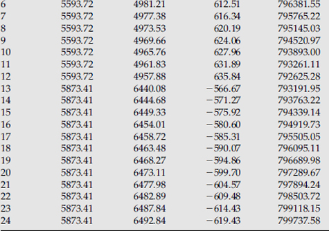
If the adjustable-rate mortgage has a payment cap, there will be a limit on how much the monthly payments can increase or decrease at the end of every period. Let us take the case of the mortgage that we studied in the preceding example. The mortgage rate for each year is as shown in Table 9.4.
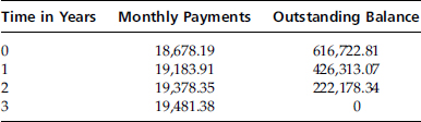
Assume there is a payment cap of 2 percent. In the absence of the cap, the monthly payments in every year and the outstanding balance at the beginning of each year will be as given in Table 9.5.
However, if there is a payment cap of 2 percent, then the monthly payment in the second year cannot exceed
![]()
The interest component in the thirteenth month will be
![]()
Table 9.4 Observed Values for LIBOR
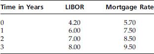
Table 9.5 Monthly Payments & Outstanding Balances
The principal repayment will therefore be only
![]()
as compared to
![]()
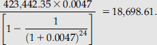
in the absence of the cap. The cap leads to a slower repayment of principal. The outstanding balance at the end of the twenty-fourth month is given by
as compared to $426,313.07 in the absence of the cap. The monthly payment in year three will therefore be
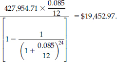
The cap for the period is
![]()
The monthly payment in year three will be $19,432.79.
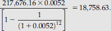
The outstanding balance at the end of the thirty-sixth month is given by
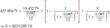
The monthly payment for year four will therefore be
Negative Amortization
There are times when a situation could arise in which the capped monthly payment is less than the monthly interest that is due for a subsequent month. If so, instead of a reduction in the outstanding balance, the deficit in the interest payment will be added to the outstanding balance, causing the principal to increase in value. This is referred to as negative amortization. We will illustrate it with the help of Example 9.3.
Consider a 30-year ARM with an initial loan amount of $800,000. The initial mortgage rate is 7.5 percent, and payments are to be made on a monthly basis. There is a payment cap of 5 percent.
The monthly installment for the first year is
The outstanding balance at the end of the first year is
![]()
Assume that the mortgage rate at the end of the year is 9.75 percent. The monthly payments in the second year in the absence of a cap would be
However, because of the cap, the payment has to be
![]()
The interest due for the thirteenth month is
![]()
There is a deficit of
![]()
This will be added to the principal. The principal at the end of the thirteenth month will be
![]()
The amortization schedule for the first two years is given in Table 9.6. The evidence of negative amortization is obvious.
Table 9.6 Illustration of Negative Amortization
Graduated-Payment Mortgage
Young home buyers may not have the disposable income required to avail a conventional fixed-rate mortgage. However, many people in this age bracket have the potential to earn substantially more in the coming years. To encourage such parties to take loans, the graduated payment mortgage was designed. Such a mortgage starts with a level of payment that steadily increases every year up to a point, and then remains steady thereafter. We will illustrate it with the help of an Example 9.4.
Mathew Thomas is being offered a mortgage loan by First National Housing Bank with the following terms. The monthly payment will increase by 5 percent every year for five years and remain constant thereafter. The mortgage rate is 9.75 percent per annum for a loan amount of $800,000. What will the payment schedule look like?
Let us denote the monthly payment for the first year by A. Then
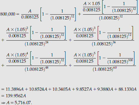
The monthly payment values for each year are given in Table 9.7.
Table 9.7 Monthly Payments for a GPM
| Year | Monthly Payment |
| 1 | 5,716.07 |
| 2 | 6,001.87 |
| 3 | 6,301.97 |
| 4 | 6,617.07 |
| 5 | 6,947.92 |
| 6-30 | 7,295.31 |
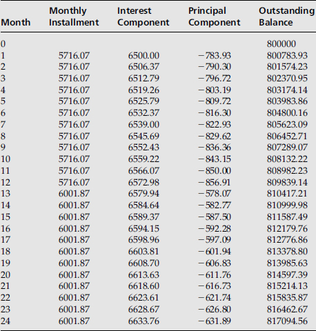
The monthly payments for the first two years are given in Table 9.8. In this case, too, there is negative amortization.
Table 9.8 Amortization Schedule for a GPM
WAC and WAM
All the mortgages that constitute the pool being securitized will not have the same mortgage rate or time to maturity. It is a common practice in the market for securitized assets to take cognizance of the weighted-average coupon (WAC) rate and the weighted-average time to maturity. The WAC of a mortgage pool is determined by weighting the mortgage rate of each loan in the pool by the principal amount outstanding. In other words, the weight for each mortgage rate is the outstanding amount of that mortgage divided by the cumulative outstanding amount of all the mortgages in the pool. Similarly, the weighted-average maturity (WAM) is found by weighting the remaining number of months to maturity of each of the loans in the pool by the principal amount outstanding. We illustrate the calculations as follows for a hypothetical pool.
Calculation of WAC and WAM
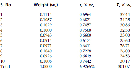
Assume that a pool consists of 10 mortgage loans. The mortgage rate for each loan and its remaining term to maturity are given in Table 9.9.
The weight to be attached to each of the mortgage rates and terms to maturity, in order to compute the WAC and the WAM, are given in Table 9.10, as are the calculated values of the two variables.
The WAC for the pool is 6.9265 percent, and the WAM is 301.07 months.
Pass-Through Securities
Mortgage loans are extremely illiquid. Besides, the lender faces significant exposure to credit risk as well as prepayment risk, so making a secondary market for whole loans is an extremely difficult proposition. However, it is possible to issue liquid debt securities that are backed by an underlying pool of mortgage loans: the cash flows stemming from the underlying loans are passed through to the holders of these debt securities, hence the name. Each holder of a pass-through security is entitled to a pro rata undivided share of each cash flow that emanates from the underlying pool, as when the home owners make monthly payments. Each monthly payment will consist of an interest component, a principal component, and potentially an additional amount on account of prepayment. Any amount that constitutes a prepayment is termed as an unscheduled principal, as opposed to the scheduled or expected principal repayment. Example 9.5 illustrates the mechanics of a pass-through.
Table 9.9 Mortgage Loans, Their Rates, and Times to Maturity
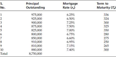
Table 9.10 Calculation of WAC and WAM
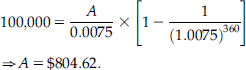
Four home loans with a principal of $100,000 each and 30 years to maturity have been pooled. The mortgage rate for two loans is 7.50 percent per annum, and the rate for the remaining two is 9.00 percent per annum. One hundred securities backed by these loans have been created. These securities have been distributed as follows: 25 to Alex, 50 to Morena, 15 to Mark, and 10 to Davena. These securities are identical in all respects, and the holder of a security is entitled to 1 percent of any cash flow that arises from the underlying loans.
The meaning of the term undivided may be understood as follows. Alex owns 25 percent of the securities, which is equivalent to 25 percent of the underlying collateral and amounts to one loan of $100,000. However, by virtue of the fact that he has 25 percent of the securities, it cannot be construed that Alex owns one underlying loan in its entirety. All that we can say is that Alex is entitled to 25 percent of each cash flow that emanates from the underlying pool.
The first month's payment for a loan with a rate of 7.50 percent is $699.21. This consists of $625 of interest and $74.21 of scheduled principal. For the loan with a rate of 9.00 percent, the first month's payment will be $804.62, which is composed of $750 of interest and $54.62 of principal.
The total cash flow from the underlying pool in the first month will be
![]()
Each of the 100 mortgage-backed securities that have been issued is entitled to $30.08 in the first month. Because Alex owns 25 securities, he will receive
![]()
By the same logic, Morena will receive $1,504.00, Mark will receive $451.20, and Davena will receive $300.80.
Assume that each of the four home owners makes an additional principal payment of $100 at end of the first month. This was not scheduled and consequently is a prepayment. The total cash flow from the underlying loans on account of this prepayment is $400. Each mortgage-backed security will receive $4 more. Because Alex has 25 securities, he will receive $100 extra, which means that his total inflow will be $852.00. By the same logic, Morena will receive $1,704.00, Mark will receive $511.20, and Davena will receive $340.80.
Cash Flows for a Pass-Through
Assume that the underlying pool consists of four loans of $100,000 each with a rate of 9 percent and 360 months to maturity. The WAC will remain constant at 9 percent, and the WAM at any point of time will be equal to the time remaining in the life of the loans. Before we can project the cash flows, we need to consider servicing and guaranteeing fees and consider the important issue of prepayments.
The cash flow that is passed through to investors in a given period will not be equal to the payment received from the underlying pool. The monthly cash flow for a pass-through is less than the monthly cash flow from the underlying loans by an amount equal to the servicing and guaranteeing fees. The coupon rate on the pass-through will be less than the mortgage rate of the underlying pool by an amount equal to the servicing and guaranteeing fees. We will assume a servicing fee of 0.5 percent per annum and a guaranteeing fee of 0.5 percent per annum. In our case, the coupon rate of the pass-through will be 8 percent.
Prepayment Conventions
It is impossible to predict the monthly cash flow stream that a pass-through holder receives with absolute certainty because the timing and amount of principal that is prepaid is subject to considerable uncertainty. Because a pass-through is a debt security, we need to project the cash flows from it in order to determine its value. Such a projection entails an assumption about the prepayment behavior of the mortgage owners over the life of the pool. The prepayment rate that is assumed is called the prepayment speed.
Single-Month Mortality Rate
The single-month mortality rate for a given month t (SMMt) is defined as
![]()
where SPt is the scheduled principal outstanding at the end of month t and Lt is the actual principal outstanding at the end of month t.
The actual principal at the end of month t is given by
![]()
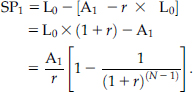
Consider a mortgage with N months to maturity and a monthly interest rate of r. The original loan balance is given by
![]()
where A1 is the scheduled monthly installment for month 1. The scheduled principal at the end of the first month is given by
The actual balance at time 1 is given by
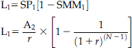
where A2 is the scheduled monthly installment for month 2.
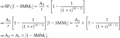
Similarly, it can be shown that
![]()
In general, the scheduled monthly installment in month t is given by
![]()
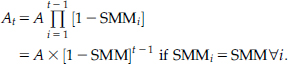
If SMM i = SMM ![]() i, then
i, then
![]()
Let us denote the monthly payment on the original principal in the absence of prepayments by A. Then we can state
In the absence of prepayments, the interest and principal components of the tth payment and the outstanding principal at the end of t periods are given by
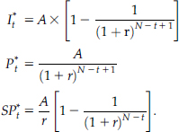
In the presence of prepayments, the actual principal outstanding at the end of t − 1 is given by
![]()
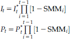
In the presence of prepayments, the interest and principal components of the tth payment are given by
![]()
and
![]()
The scheduled principal at the end of the tth period is given by
![]()
We know that
![]()
and
![]()
The actual principal at the end of t periods is given by
![]()
Therefore,
![]()
Example 9.6 gives a detailed illustration of cash-flow calculations for a pass-through security.
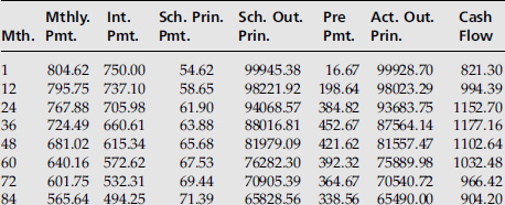
Consider a pool of four mortgage loans. Each loan has an outstanding principal of $100,000 and 24 months to maturity. The mortgage rate is 9 percent for each loan. The servicing fee is 0.5 percent of the outstanding balance, and the guarantor's fee is also 0.5 percent of the outstanding balance. The SMM is 2.5 percent for all the months.
The cash flows in the absence of prepayments are given in Table 9.11.
Table 9.11 Amortization Schedule in the Absence of Prepayments

Mthly. Pmt. = monthly payment; Serv. Fee = servicing fee; Grnt. Fee = guaranteeing fee; Net. Int. = net interest; Prin. Pmt. = principal payment; Out. Prin. = outstanding principal
Analysis of Amortization in the Absence of Prepayments
Consider the entries for the first month in Table 9.11. The principal outstanding at the beginning of the month is $400,000. The monthly payment due is given by
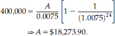
![]()
The guarantee fee for every month is the same as the servicing fee. The net interest to be passed through for the first month is
![]()
The principal payment for the month is
![]()
The total cash flow for the holders of the pass-through securities is
![]()
Let us consider the repayment schedule assuming that the SMM is 2.5 percent for all months.
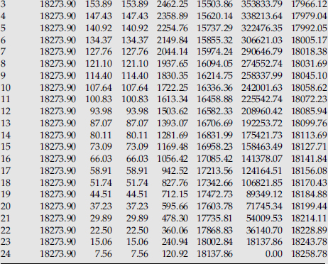
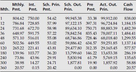
A Revised Analysis (Assuming Prepayments)
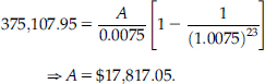
Let us analyze the entries in Table 9.12. The payment for the first month is the same as in the preceding case that is $18,273.90. The servicing and guaranteeing fees are also the same as those obtained previously because they are based on the same outstanding principal: $400,000. The net interest to be passed through is $2,666.67, which is the same as the value obtained in the absence of prepayments. The scheduled outstanding balance at the end of the first month is
![]()
We have assumed a constant SMM of 2.50 percent, so the prepayment at the end of the first month is 0.025 × $384,726.10 = $9,618.15. The actual outstanding principal at the end of the first month is then
![]()
The total cash flow for the month for the pass-through holders is the sum of the net interest plus the scheduled principal payment plus the prepayment, which in this case is
Let us consider the entries for the second month. The total payment for the month is given by
The servicing and guaranteeing fees for the second month are
![]()
The net interest for the second month is
![]()
The scheduled principal payment for the month is
![]()
The scheduled outstanding principal at the end of the month is
![]()
The prepayment at the end of the month is 0.025 × $360,104.21 = $9,002.61. The actual outstanding principal at the end of the second month is therefore
![]()
The cash flow for the month that is directed toward the pass-through holders is
![]()
The analysis can be extended along similar lines to the remaining months.
Table 9.12 Amortization Schedule in the Presence of Prepayments
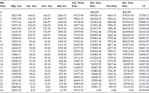
Mly. Pmt. = monthly payment; Ser. Fee = servicing fee; Grn. Fee = guaranteeing fee; Net. Int. = net interest; Sch. Prin. Pmt. = scheduled principal payment; Sch. Out. Prin. = scheduled outstanding principal; Pre Pmt. = prepayment; Act. Out. Prin. = actual outstanding principal; CF = cash flow
Average Life
Unlike a bond that repays its principal in the form of a bullet payment at maturity, a pass-through security returns a part of its principal every month. It is a common practice to compute the average life of a pass-through security. Let PCFt be the total principal received at time t. PCFt is the sum of the scheduled principal received at time t and the prepayment received at the same point in time. The average life may be defined as

In the case of the pass-through previously discussed, the average life in the absence of prepayments is 12.8578 months, or 1.0715 years. However, when we assume an SMM of 2.50 percent per month, the average life declines to 10.6677 months, which is equivalent to 0.8890 years. The higher the prepayment speed that is assumed, the shorter the average life of the security.
Cash-Flow Yield
The cash-flow yield for a pass-through is the internal rate of return (IRR) computed using the projected cash-flow stream. The result is a monthly rate, which is usually converted to a bond equivalent yield (BEY) to facilitate comparisons with conventional debt securities. If we denote the IRR as im, where im denotes a monthly rate, then the bond equivalent yield may be expressed as
![]()
Example 9.7 presents the cash flow yield and the bond equivalent yield for a mortgage-backed security under various pre-payment assumptions.
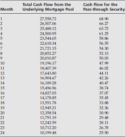
Assume that the pool of four mortgages with a principal of $100,000 each and with a coupon of 9 percent is securitized, and 400 securities are issued. The par value of each security is $1,000, and each security will be eligible for 1/400 of each cash flow emanating from the underlying pool. The monthly cash flows for each security, assuming an SMM of 2.50 percent, are given in Table 9.13.
Table 9.13 Cash Flows for a Security with a Par Value of $1,000
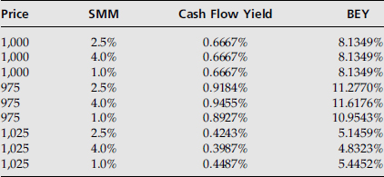
The cash-flow yield and the corresponding bond equivalent yield for this security are given as follows for three different price scenarios, and three assumed prepayment speeds in each case.
From Table 9.14, the BEY for a pass-through is inversely related to the price of the security, as is the case for a conventional debt security. If the security is priced at par, the cash-flow yield is equal to the coupon rate, irrespective of the rate that is assumed for prepayment.
Conditional Prepayment Rate
To project the cash flows from a pass-through, we need to make an assumption about the prepayment behavior. The prepayment rate that is assumed for a pool of mortgages is called the conditional prepayment rate (CPR). The term conditional connotes that the rate is conditional on the remaining balance in the pool.
The CPR corresponding to the assumed prepayment speed has to be converted to the equivalent SMM. The formula for conversion is the following:
![]()
The rationale for this formula is the following. Assume that the SMM is constant for a year. Let SP*12×N be the scheduled principal at the end of year N in the absence of prepayments, and let L12×N be the actual principal at the end of the Nth year. We know that
![]()
If we denote the corresponding annual prepayment rate as CPR, then
![]()
![]()
PSA Prepayment Benchmark
The Public Securities Association (PSA) prepayment benchmark is expressed as a monthly series of annual prepayment rates.2
The PSA benchmark assumes that prepayment rates are lower for newly originated mortgages and will then speed up as the mortgages become seasoned. It has been observed that home owners are less likely to move in the initial years of the loan. They are also less likely to refinance or make large unscheduled principal repayments. The PSA benchmark assumes that the prepayment rate will steadily increase for the first 30 months of the loan and then stabilize thereafter.
The benchmark assumes the following CPR for 30-year mortgages:
- CPR of 0.2 percent for the first month;
- An increase of 0.2 percent per month for the next 30 months until it reaches 6 percent; and
- 6 percent for the remaining years.
This benchmark is called 100 percent PSA or 100 PSA.
Let t be the number of months after the mortgage was originated.
![]()
Sample calculations for the 100 PSA benchmark are given as follows:
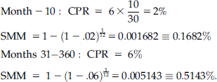
Slower or faster prepayment speeds are referred to as a percentage of the standard PSA benchmark. For example, 50 PSA means one-half of the CPR of the PSA benchmark, and 150 PSA means 1.5 times the CPR of the PSA benchmark.
The case of 150 PSA, the SMM may be calculated as follows:
It should be noted that 150 PSA does not mean that the SMM for a month is 1.5 times the SMA for the same month under the 100 PSA assumption. It is the CPR for the month that is 1.5 times the CPR under the 100 PSA assumption.
Example 9.8 illustrates the cash flows from a pass-through under the assumption of 100 PSA.
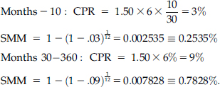
Consider a pass-through backed by a single loan of $100,000 with 360 months to maturity and a mortgage rate of 9 percent per annum. Assume there are no servicing or guaranteeing fees. The projected cash flows assuming 100 PSA are given in Table 9.15.
The average life of the pass-through is 12.08 years.
Table 9.15 Cash Flows Assuming 100 PSA
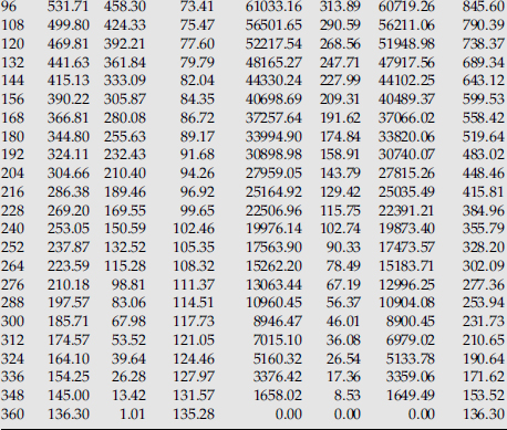
Mth. = month; Mthly. Pmt. = monthly payment; Int. Pmt. = interest payment; Sch. Prin. Pmt. = scheduled principal payment; Sch. Out. Prin. = scheduled outstanding principal; Pre. Pmt. = prepayment; Act. Out. Prin. = actual outstanding principal
Analysis of Cash Flows Assuming 100 PSA
Consider the data for the first month. The monthly payment is given by
The interest component for the first month is
![]()
The scheduled outstanding principal at the end of the month is
![]()
The CPR for the first month is 0.2 percent. So the SMM is
![]()
The prepayment for the month is
![]()
The actual outstanding principal at the end of the first month is
![]()
The cash flow for the pass-through is
![]()
Example 9.9 illustrates the cash flows from a pass-through under an assumption of 200 PSA.
Consider a pass-through backed by a single loan of $100,000 with 360 months to maturity and a mortgage rate of 9 percent per annum. Assume that there are no servicing or guaranteeing fees. The projected cash flows assuming 200 PSA are given in Table 9.16.
The average life of the pass-through is eight years. As can be seen, the more rapid prepayments lead to a reduction in the average life of the security.
Table 9.16 Cash Flows Assuming 200 PSA
Mth. = month; Mthly.Pmt. = monthly payment; Int. Pmt. = interest payment; Sch. Prin. Pmt. = scheduled principal payment; Sch. Out. Prin. = scheduled outstanding principal; Pre. Pmt. = prepayment; Act. Out. Prin. = actual outstanding principal
Collateralized Mortgage Obligations
In the case of a pass-through, there is only one class of security that is issued, and every security is entitled to the same undivided share of the cash flows from the underlying pool. The feature of such securities is that prepayments have the same implications for all the security holders.
In real life, however, investors differ with respect to the prepayment exposure and the average security life sought by them. The securitization process can take these preferences into account by creating multiple classes of securities or what are referred to in the parlance of mortgage-backed securities as tranches. There are clearly specified rules as to how the cash flows from the underlying pool are to be directed to the holders of the various tranches. Such securities, with multiple tranches, are referred to as collateralized mortgage obligations (CMOs). We will introduce the concept by studying a very simple CMO structure known as a sequential pay CMO.
Table 9.17 Amortization for Tranche A
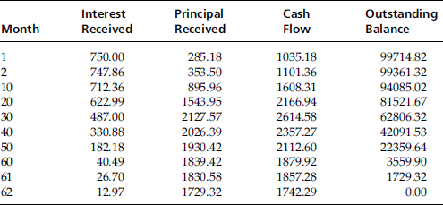
Sequential Pay CMO
Assume that a pool of mortgages consists of four loans with a principal of $100,000 each. Each loan has a maturity of 360 months and a mortgage rate of 9 percent. The average life of a pass-through, backed by such loans, under the assumption of 100 PSA is 12.08 years, as we have just seen.
Assume that instead of creating a single type of security like a pass-through, four types of securities known as tranches A to D are created. All principal payments from the underlying pool, both scheduled and unscheduled, will first go to tranche A. During this time, the remaining tranches will continue to earn interest on the outstanding principal. Once tranche A is fully paid off, all subsequent principal payments, scheduled and unscheduled, will be directed to the holders of tranche B. Once again, while tranche B is being paid off, holders of tranches C and D will get interest on their outstanding principal. Extending the logic, the redemption of tranche B will see further principal payments being directed to tranche C, with holders of tranche D getting only the interest due. Finally, once tranche C securities are retired, all further principal payments will be directed to the holders of tranche D.
Let us assume that one security is issued for each tranche, with a face value of $100,000, and that there are no servicing or guaranteeing fees. The cash-flow schedules for the four tranches are given in Tables 9.17 to 9.20.
Table 9.18 Amortization for Tranche B
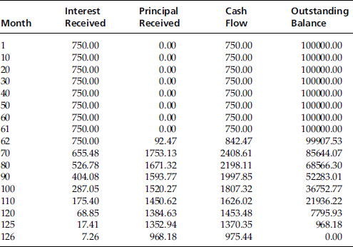
Table 9.19 Amortization for Tranche C
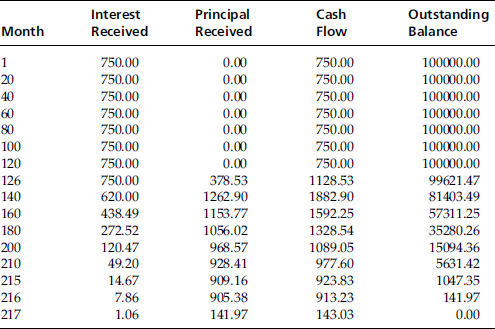
Table 9.20 Amortization for Tranche D
Analysis of Amortization for Tranche A of a Sequential Pay CMO
Consider the first month. The scheduled principal that is received from the underlying pool is
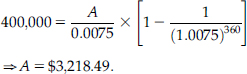
The interest component for the month is
![]()
The scheduled principal for the month is $3,218.49 − $3,000 = $218.49. This will be directed toward tranche A.
The prepayment for the month is
![]()
This will also be directed to tranche A. The total principal received by tranche A is $218.49 + $66.68 = $285.17.
The interest receivable by this security for the month is
![]()
The total cash flow received by tranche A in the first month is
![]()
Consider the second month. The monthly payment received from the underlying pool is
The interest component for the month is
![]()
The scheduled principal for the month is
![]()
The prepayment for the month is
![]()
So the total principal for the month is $220.09 + $133.41 = $353.50.
The entire amount will be directed toward tranche A. The interest receivable by this tranche for the second month is given by
![]()
The total cash flow that is directed toward tranche A at the end of the second month is $747.86 + $353.50 = $1,101.36.
At the end of the sixty-first month, tranche A has an outstanding principal of $1,729.32. The total principal from the underlying pool at the end of the sixty-second month is $1,821.79. Of this, $1,729.32 will be directed to tranche A. The balance of $92.47 will be paid to tranche B. The total cash flow received by tranche A in the sixty-second month is
![]()
Analysis of Amortization for Tranche B
Let us turn our attention to tranche B. For the first sixty-one months, tranche B will receive only interest on the outstanding principal of $100,000, which amounts to $750 per month. In the sixty-second month, this tranche receives $92.47 by way of principal payment as previously explained. The total cash flow for this month is $750 + $92.47 = $842.47. The outstanding principal at the end of the month is $100,000 − $92.47 = $99,907.53. In the 125th month, the outstanding principal for this tranche is $968.18. In the 126th month, the underlying pool makes a total principal payment of $1,346.71. In this month, tranche B receives $7.26 worth of interest and $968.18 of principal, which amounts to a total cash flow of $975.44. The excess principal—that is, $1,346.71 − $968.18 = $378.53—is directed to tranche C.
Analysis of Amortization for Tranche C
Let us consider tranche C. Until the 125th month, this tranche receives a monthly cash flow of $750, which represents the interest on an outstanding principal of $100,000. In the 126th month, there is a principal repayment of $378.53, as previously explained. The total cash flow for this month is therefore $1,128.53. At the end of 216 months, there is an outstanding principal of $141.97. So in the 217th month, this tranche receives an interest payment of $1.06. In this month, the total principal received from the underlying pool is $901.61. After paying $141.97 to tranche C, the excess of $759.64 is directed toward tranche D.
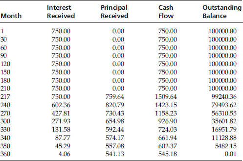
Analysis of Amortization for Tranche D
Finally, let us analyze the last tranche. Tranche D receives interest on the initial outstanding principal until month 216 that amounts to $750 per month. In month 217, it receives a principal payment of $759.64 as previously explained. The tranche is fully paid off in month 360.
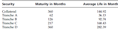
The average life of the collateral as calculated for a pass-through security based on the pool is 12.08 years. However, each tranche of the CME has a different maturity and average life. The details are given in Table 9.21.
Table 9.21 Maturity and Average Life of the Securities
Extension Risk and Contraction Risk
Pass-through securities and CMOs expose investors to prepayment risk. In a declining interest-rate environment, prepayments impact security holders in two ways. First, since they are debt securities, we would expect the price of such securities to rise in a scenario where rates are declining. However, in the case of mortgage-backed securities, holders of underlying bonds are likely to prepay and refinance at a lower rate when market rates go down. The overall result is price compression: the rise in price will not be as large as in the case of plain vanilla bonds. The second adverse consequence for holders of such securities is, of course, reinvestment risk, as is the case for all debt holders. In other words, cash flows that are received in a declining interest-rate environment have to be reinvested at lower rates of interest. The risk from these two adverse consequences is termed contraction risk.
Let us consider a rising interest-rate environment. We would expect the prices of mortgage-backed securities to fall. However, unlike in the case of plain vanilla bonds, principal payments are likely to slow down because holders of underlying mortgage loans are less likely to refinance when mortgage rates are rising. This will exacerbate the anticipated price decline. In such a situation, the security holders would like prepayments to be high because it would afford them an opportunity to reinvest larger amounts at high rates of interest. The adverse impact for mortgage-backed securities in a rising interest-rate environment is termed extension risk.
Accrual Bonds
In the case of the sequential pay CMO that we just studied, every tranche receives interest every month, based on the principal outstanding for that particular tranche at the beginning of the month. However, many sequential pay CMO structures do not require that every tranche be paid interest every month based on the outstanding principal. In the case of a sequential pay CMO with an accrual bond (also termed a Z bond3), however, the Z bond will not receive any monthly interest until the previous tranches are fully retired. Therefore, the interest for the Z bond will accrue and be added to its original principal (negative amortization) until the other classes of the CMO have been paid off. In the months before the retirement of the penultimate tranche, the interest that would otherwise have been paid to the Z bond is directed to the tranche that is receiving principal at that point in time, and it helps speed up the repayment of principal.
Let us consider a CMO in which tranches A, B, and C are as specified in the preceding illustration. However, the last tranche is an accrual bond. The inclusion of the Z bond will reduce the maturity as well as the average life of each of the three earlier tranches. Tables 9.22 to 9.25 illustrate the amortization schedules of the various tranches of a CMO that includes a Z-bond.
Table 9.22 Amortization for Tranche A in the Presence of a Z-bond
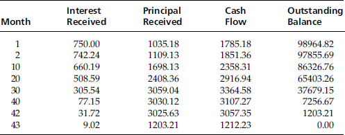
Table 9.23 Amortization for Tranche B in the Presence of a Z-bond
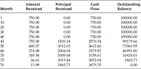
Table 9.24 Amortization for Tranche C in the Presence of a Z-bond
Analysis of Cash Flows for a CMO with an Accrual Bond
The cash flows from the underlying pool at the end of the first month are as follows.
![]()
The outstanding principal for each of the four tranches is $100,000. Tranches A, B, and C will therefore receive an interest payment of $750 for the month. The accrual bond will not receive any interest. Tranche A will receive the following amount by way of principal payment
![]()
The total cash flow for this tranche is $750 + $1,035.18 = $1,785.18. The outstanding principal at the end of the first month is $100,000 − $1,035.18 = $98,964.82.
Because the Z bond does not receive any interest during the month, there will be negative amortization. The outstanding principal for this bond at the end of the first month is $100,750.
Let us consider the second month. The cash flows from the underlying pool are as follows: interest = $2,997.86, scheduled principal = $220.09, prepayment = $133.41. Tranche A has an outstanding principal of $98,964.82. The interest for the month for this tranche is
Table 9.25 Amortization for the Z-Bond

![]()
Tranches B and C will each receive $750 for the month by way of interest because there has been no principal repayment. The principal repayment that is directed at tranche A for this month is
![]()
The outstanding principal at the end of the second month is therefore $98,964.82 − $1,109.12 = $97,855.70.
Tranche Z will not receive any cash flow during the month. The interest due is
![]()
The outstanding principal at the end of the second month is $100,750 + $755.63 = $101,505.63.
Let us turn to the forty-third month. The cash flows from the underlying collateral are as follows: interest = $2,535.51, scheduled principal = $259.71, prepayment = $1,737.35.
The outstanding principal for tranche A at the end of the forty-second month is $1,203.21. This tranche will receive a cash flow of $1,203.21 × (1.0075) = $1,212.23. With this, tranche A is retired.
Tranches B and C are entitled to an interest payment of $750 each. The principal payment that is received by tranche B during this month is
![]()
The total cash flow that is received by tranche B at the end of this month is $2,570.34. The outstanding principal is $100,000 − $1,820.34 = $98,179.66.
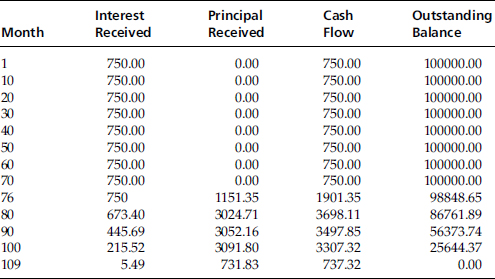
Similarly, tranche B is retired at the end of 76 months and tranche C at the end of 109 months. From the 109th month onward, the Z bond starts receiving repayments of principal. The outstanding principal for the bond at the end of month 108 is $224,112.42. In the 109th month, the tranche receives an interest payment of $224,112.42 × 0.0075 = $1,680.84. It also receives a principal payment of $725.59 that reduces the outstanding principal to $223,386.83. The tranche is fully paid off at the end of the 360th month.
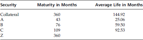
From Table 9.26, the average life of each of the three tranches has reduced because of the presence of the Z bond, which appeals to investors who are primarily concerned with the specter of reinvestment risk. Because such bonds do not entail the receipt of any cash flows until all the other classes are fully retired, reinvestment risk is totally eliminated until the Z bond starts receiving its first cash flow.
Table 9.26 Maturity and Average Life of the Securities in the Presence of a Z Bond
Floating-Rate Tranches
Floating-rate bonds can be created from a fixed-rate tranche. We will illustrate this using tranche C in the preceding illustration, which has a par value of $100,000 and a 9 percent coupon. To create a floater, we have to simultaneously create an inverse floater.4 The cumulative principal of the two tranches will be $100,000 in this case. There is no rule as to what the principal values of the respective tranches should be as long as their combined par value is $100,000.
Let us assume that the benchmark for the two tranches is the three-month LIBOR and that we wish to create a floater with a par value of $60,000 and an inverse floater with a par value of $40,000. The coupon on the floater is LIBOR + m basis points, whereas that for the inverse floater is C − L × LIBOR.
It is a common practice to specify the coupon for an inverse floater as
![]()
C is the cap or maximum interest on the inverse floater, and L is referred to as the coupon leverage. The concept of a cap can be easily understood. The lower limit for LIBOR is zero. The upper limit for the coupon on the inverse floater is C. The coupon leverage measures the rate of change of the coupon of the inverse floater with respect to the benchmark.
We know that the total annual interest available is 9 percent of 100,000, or 9,000. This is also the maximum interest available for the floating tranche. The cap on the floater is 9,000 ÷ 60,000 = 15 percent. The ratio of floaters to inverses is 3:2, which implies that the coupon leverage for the inverse floater is 1.50. If we assume that the coupon on the floater is LIBOR + 150 bp, then the minimum coupon on the floater is 1.50 percent, which would be the case if LIBOR was zero. The minimum interest on the floater is $60,000 × 0.015 = $900. So the maximum interest for the inverse floater is $9,000 − $900 = $8,100. The cap on the inverse is therefore 8,100 ÷ 40,000 = 0.2025 = 20.25 percent. We can therefore express the coupons of the two tranches as
The weighted-average coupon is
![]()
If LIBOR is 7.50 percent, the weighted average will be
![]()
Notional Interest Only Tranche
Let us go back to the sequential pay CMO we studied earlier. We assumed that the underlying mortgages had a coupon rate of 9 percent and that each of the four tranches that we created also had a coupon of 9 percent. Each tranche of a CMO will have a different coupon rate, and there will be an excess representing the difference between the interest on the underlying collateral and the coupons on the various tranches. Therefore, it is a common practice to create a tranche that is entitled to receive only the excess coupon interest.5 Such tranches are referred to as notional interest-only securities.
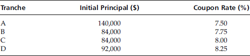
We will assume that the underlying collateral has a coupon of 9 percent and that the four tranches created from it have coupon rates as shown in Table 9.27.
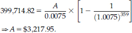
Consider tranche A. It pays a coupon of 7.50 percent, whereas the coupon on the collateral is 9 percent. There is excess interest of 1.50 percent. Let us assume that we wish to create a notional interest-only security with a coupon of 8.40 percent. To find the notional amount on which the interest payable to this security will be calculated, we proceed as follows. An excess interest of 1.50 percent on $140,000 worth of principal can be used to pay an interest of 8.40 percent on a principal amount of $25,000.
Table 9.27 Coupon Rates for a Sequential Pay CMO
Similarly, in the case of tranche B, an excess interest of 1.25 percent on a principal amount of $84,000 can be used to pay an interest of 8.40 percent on a principal of $12,500. Tranche C, using the same logic, generates excess interest to support $10,000 worth of principal, and the last tranche is capable of servicing a principal of $8,214.2850. The excess interest generated can service a bond with a principal of 25,000 + 12,500 + 10,000 + 8,214.285 = $55,714.285. This is the notional principal for the tranche that is scheduled to receive the excess interest. The term notional connotes that this principal amount is used merely to compute the interest payable to this class for the month and that the principal per se is not repaid.
The contribution of a tranche to the notional principal is in general given by the following formula.
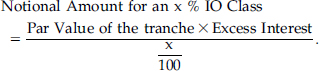
In the case of tranche A in the preceding illustration,
![]()
For the first month, the IO class will receive a cash flow of
![]()
Let us assume a prepayment speed of 100 PSA. The principal paid to tranche A at the end of the first month will be $285.18. This will reduce the outstanding principal for this tranche to 140,000 − 285.18 = $139,714.82. The contribution of this tranche to the notional principal for the second month is
![]()
The contributions of the other tranches will not be affected. For the second month, the notional IO class will receive interest on a principal of
![]()
The interest for this tranche for the second month will be
![]()
Interest-Only and Principal-Only Strips
Stripped mortgage-backed securities can be created by either directing all the principal or all the interest to a particular class. The security that is scheduled to receive only the principal is referred to as the principal-only (PO)class. The other security is termed the interest-only (IO) class.
Let us first consider the PO class. The yield obtained by the security holder will depend on the speed with which the underlying pool generates prepayments. The more quickly that prepayments are received, the greater the rate of return for holders of such securities. In the case of IO class holders, however, the desire is to have slow prepayments because such securities do not receive any principal payments, and the income (which is exclusively by way of interest payments) will be higher, the larger the outstanding balance on the underlying pool (which is tantamount to a slower prepayment rate).
PAC Bonds
PAC is an acronym for planned amortization class. In the case of such bonds, if the prepayment pattern falls within a prespecified range, then the cash flows received by the security are known.
PAC bonds are not created in isolation. They are accompanied by a category of bonds that are termed support bonds. It is this category that absorbs the prepayment risk, thereby protecting the PAC bonds against extension risk as well as contraction risk.
To create a PAC bond, we need to specify a range of prepayment speeds. These are referred to as PAC collars. The PAC schedule lists the principal amount payable to the PAC bondholders if the prepayment speed is within the range provided by the lower and upper PAC collars. The schedule is obtained by taking the lower of the principal cash flows generated by the lower collar and the upper collar. Consider the Example 9.10.
A pool of four mortgage loans of $100,000 each is used to create a PAC bond and a support bond. The lower PAC collar is 100 PSA, and the upper collar is 250 PSA. Table 9.28 lists the principal payments from the underlying pool, assuming four different pre-payment speeds between the lower and upper collars.
Table 9.28 Principal Payments for a 100 PSA to 250 PSA Range
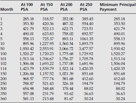
The sum total of the principal payments per the PAC schedule is $278,088.22. This represents the maximum principal for the PAC bonds. For our illustration, we have assumed that the PAC bond has a principal of $277,500, whereas the support bond has a principal of $122,500
Analysis of Principal Payments for Speeds between the Lower and Upper PAC Collars
Until the 113th month, the lowest principal payment is obtained under the assumption of 100 PSA. From the 114th month onward, the lowest principal payment is observed under the assumption of 250 PSA.
Table 9.29 Principal Payments at 150 PSA
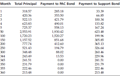
We will first consider the prepayment scenario corresponding to 150 PSA as shown in Table 9.29.
Analysis (The Case of 150 PSA)
Until the 344th month, the total principal received is in excess of the amount required to satisfy the PAC schedule. The difference is therefore directed to the support bond. In the 344th month, the outstanding amount on the PAC bond is $13.53. The total principal received is $243.49. The excess of $229.96 is directed to the support bond. In subsequent months, because the PAC bond has been fully paid off, the entire principal received is directed to the support bond. The average life of the PAC bond is 98.13 months, and that for the support bond is 156.69 months.
Let us consider the prepayment scenario corresponding to 250 PSA as shown in Table 9.30.
Analysis (The Case of 250 PSA)
Until the 113th month, the principal payment, scheduled as well as unscheduled, from the underlying collateral and based on the assumption of 250 PSA, is greater than the amount required to be directed toward the PAC bond on the basis of the PAC schedule. Until the 113th month there is a cash inflow for the support bond. From the 114th until the 343rd month, the total principal payment is just adequate to satisfy the PAC schedule. The payment directed toward the support bond during these months is nil. In the 344th month, the total principal received is $40.97. The outstanding balance for the PAC bond is $13.53. The payment for the support bond is $27.44. Because the PAC bonds are fully paid off at this stage, in subsequent months all principal received is directed to the support bond.
Table 9.30 Principal Payments at 250 PSA
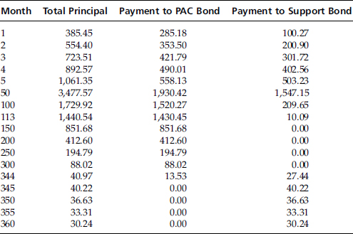
As to be expected, the average life of the PAC bond continues to remain at 98.13 months. However, the average life of the support bond falls to 44.07 months. This highlights the protection provided by the support bond. In this, case the entire impact of contraction resulting from faster prepayment is absorbed by the support bond.
Let us consider the prepayments at 0 PSA or, in other words, a situation corresponding to no prepayments as shown in Table 9.31.
Analysis (The Case of 0 PSA)
Until the 161st month, the total principal received is inadequate to satisfy the PAC schedule. The entire principal received is directed toward the PAC bond, and the support bond does not receive any payment. The deficit with respect to the PAC schedule is accumulated until the end of the 161st month when it reaches a value of $164,228.15. From the 162nd until the 314th month, the entire principal is directed to the PAC bond, and the deficit is steadily reduced. At the end of the 314th month, the cumulative deficit is $735.60. The scheduled payment for the PAC bond for the 315th month is $68.43. A cash flow of $804.03 is directed to the PAC bond. The total cash flow for the month is $2,282.34. Thus, $1,478.31 is directed to the support bond. From here on until the 344th month, the principal received is in excess of what is required to satisfy the PAC schedule, and the excess is directed toward the support bond. The principal outstanding for the PAC bond as of the end of month 343 is $13.53. The principal received in month 344 is $2,834.56. Thus, $2,821.03 is directed to the support bond at the end of this month. For all subsequent months, the entire principal received is directed to the support bond. The average life of the PAC bond is 214.83 months, and that of the support bond is 339.10 months. Although slower prepayment increases the average life of the bonds, the impact on the support bond, as is to be expected, is greater than the impact on the PAC bond.
Table 9.31 Principal Payments at 0 PSA
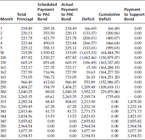
Table 9.32 Principal Payments at 400 PSA
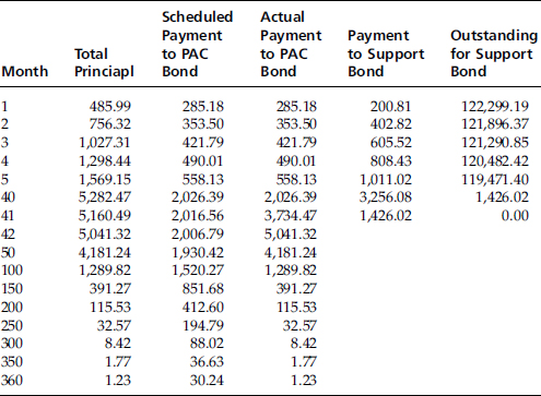
Finally, let us consider a scenario corresponding to 400 PSA as shown in Table 9.32.
Analysis (The Case of 400 PSA)
Until the fortieth month, the total principal received is in excess of what is required by the PAC schedule, so the excess is directed to the support bond. As of the end of the fortieth month, the outstanding principal on the support bond is $1,426.02. In the forty-first month, this amount is directed to the support bond, and the balance is directed to the PAC bond. With this, the support bond is fully paid off. In subsequent months the entire principal received is directed to the PAC bond. The average life of the PAC bond is 70.43 months, and that of the support bond is 24.78 months.
Agency Pass-Throughs
The U.S. federal government has set up three agencies to guarantee mortgage-backed securities. Pass-throughs guaranteed by such agencies are referred to as agency pass-throughs as compared to private-label pass-throughs, which are issued by nongovernment entities such as commercial banks and savings-and-loan associations. The three federal agencies are the Government National Mortgage Association (Ginnie Mae), the Federal National Mortgage Association (Fannie Mae), and the Federal Home Loan Mortgage Corporation (Freddie Mac).
Ginnie Mae
Ginnie Mae was established in 1968. Unlike the other two federal agencies, Ginnie Mae is fully owned by the U.S. government. Ginnie Mae securities, like other Treasury securities such as T-bonds, are backed by the full faith and credit of the federal government.
Note that Ginnie Mae as an organization neither originates nor acquires and pools mortgage loans and nor does it issue securities. What happens is that private institutions that have been approved by Ginnie Mae pool home loans and issue mortgage-backed securities that have the guarantee of Ginnie Mae. The guaranty from Ginne Mae ensures that holders of the pass-throughs receive timely payment of principal and interest. If a borrower fails to make the required payment on a mortgage on time, then the issuer is expected to use its own funds to ensure that the security holders receive timely payment. If an issuer is unable to ensure that payments are made per schedule, then Ginnie Mae will step in to make the required payment to the security holders. This is the essence of the guaranty provided by Ginnie Mae.
Ginnie Mae guarantees securities backed by single-family and multi-family loans that are insured by U.S. government agencies. These are the Federal Housing Administration (FHA), the Department of Agriculture, the Department of Veterans Affairs, and the Office of Public and Indian Housing.
Ginnie Mae has two programs: the Ginnie Mae I MBS Program, for the issuance of securities backed by single-family or multifamily loans, and the Ginnie Mae II MBS program for the issuance of securities backed by single-family loans. In the case of Ginnie Mae I, all loans must bear the same rate of interest, with certain exceptions. However, in the case of Ginnie Mae II, the interest rates for a pool of mortgages may vary across loans. All Ginnie Mae I securities must bear a fixed rate of interest, whereas some Ginnie Mae II securities may bear an adjustable interest rate. The minimum pool size for Ginnie Mae I is US$1 million. Payment to pass-through holders is made on the fifteenth of each month. For Ginnie Mae II securities, the minimum pool size is US$250,000 for multilender pools and US$1 million for single-lender pools. Payment to holders is made on the twentieth of each month.
Fannie Mae
Fannie Mae was founded in 1938 at a time when the U.S. economy was coming to terms with the Great Depression. In 1968, it was set up as a shareholder-owned corporation by the U.S. Congress. Fannie Mae and Freddie Mac are referred to as government-sponsored enterprises (GSEs). They are referred to as quasi-government organizations because, although they are essentially private, they were set up by Congress. Most people believe that securities issued by Fannie Mae and Freddie Mac carry an implicit federal government guarantee; that is, although there is no explicit guarantee from the government from the standpoint of the credit risk of securities issued by the GSEs, it is believed that the government will inevitably bail them out in adverse circumstances, because they are considered economically too important to be allowed to fail. This belief has been reinforced by the bailout of these organizations during the recent subprime crisis.
Fannie Mae buys mortgage loans and securitizes them for sale to investors in the secondary mortgage market. To reiterate, unlike the case of Ginnie Maes, the federal government does not ensure timely payment of principal and interest on Fannie Mae securities. The guarantee on such securities is provided by Fannie Mae itself.
Freddie Mac
Freddie Mac is a GSE set up by Congress to compete with Fannie Mae. Like the former, it also pools loans and securitizes them. As in the case of Fannie Mae securities, holders of Freddie Mac securities are provided an assurance from Freddie Mac from the standpoint of timely payment of principal and interest. There is no explicit guarantee from the federal government.
Endnotes
1. The monthly income should be taken as the take-home salary and not as the cost to company (CTC).
2. This model was developed by the Public Securities Association, which was subsequently renamed the Bond Market Association (BMA). In 2006, the BMA merged with the Securities Industry Association to form the Securities Industry and Financial Markets Association (SIFMA). However, the prepayment benchmark is still referred to as the PSA benchmark.
3. Because of its similarities with a zero-coupon bond.
4. Although the coupon of a floating-rate bond moves up and down with the corresponding changes in the benchmark, the coupon of an inverse floater moves inversely with the benchmark. An inverse floater may have its coupon specified as 10% LIBOR. If the LIBOR rises, the coupon falls and vice versa.
5. Note that this tranche is not entitled to any principal payments.