Search in book...
Toggle Font Controls
Create new playlist

Name your new playlist

Playlist description (optional)
Sign In

Email address

Password

Forgot Password?

or

Continue with Facebook

Continue with Google
Sign Up

Full Name

Email address

Confirm Email Address

Password

or

Continue with Facebook

Continue with Google

7
Estimating GARCH Models by Quasi‐Maximum Likelihood

The quasi‐maximum likelihood (QML) method is particularly relevant for GARCH models because it provides consistent and asymptotically normal estimators for strictly stationary GARCH processes under mild regularity conditions, but with no moment assumptions on the observed process. By contrast, the least‐squares methods of the previous chapter require moments of order 4 at least.

In this chapter, we study in details the conditional QML method (conditional on initial values). We first consider the case when the observed process is pure GARCH. We present an iterative procedure for computing the Gaussian log‐likelihood, conditionally on fixed or random initial values. The likelihood is written as if the law of the variables η _t were Gaussian (we refer to pseudo‐ or quasi‐likelihood), but this assumption is not necessary for the strong consistency of the estimator. In the second part of the chapter, we will study the application of the method to the estimation of ARMA–GARCH models. The asymptotic properties of the quasi‐maximum likelihood estimator (QMLE) are established at the end of the chapter.

7.1 Conditional Quasi‐Likelihood

Assume that the observations ε₁, …, ε_n constitute a realisation (of length n ) of a GARCH(p, q) process, more precisely a non‐anticipative strictly stationary solution of

7.1

where (η _t) is a sequence of iid variables of variance 1, ω ₀ > 0, α _0i ≥ 0 (i = 1, …, q), and β _0j ≥ 0 (j = 1, …, p). The orders p and q are assumed known. The vector of the parameters

7.2

belongs to a parameter space of the form

7.3

The true value of the parameter is unknown, and is denoted by

To write the likelihood of the model, a distribution must be specified for the iid variables η _t . Here we do not make any assumption on the distribution of these variables, but we work with a function called the (Gaussian) quasi‐likelihood, which, conditionally on some initial values, coincides with the likelihood when the η _t are distributed as standard Gaussian. Given initial values to be specified below, the conditional Gaussian quasi‐likelihood is given by

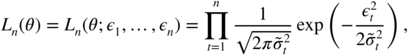
where the are recursively defined, for t ≥ 1, by

7.4

For a given value of θ , under the second‐order stationarity assumption, the unconditional variance (corresponding to this value of θ ) is a reasonable choice for the unknown initial values:

7.5

Such initial values are, however, not suitable for IGARCH models, in particular, and more generally when the second‐order stationarity is not imposed. Indeed, the constant (7.5) would then take negative values for some values of θ . In such a case, suitable initial values are

7.6

7.7

A QMLE of θ is defined as any measurable solution of

Taking the logarithm, it is seen that maximising the likelihood is equivalent to minimising, with respect to θ,

7.8

and is defined by (7.4). A QMLE is thus a measurable solution of the equation

7.9

It will be shown that the choice of the initial values is unimportant for the asymptotic properties of the QMLE. However, in practice this choice may be important. Note that other methods are possible for generating the sequence ; for example, by taking , where the c _i(θ) are recursively computed (see Berkes, Horváth, and Kokoszka 2003b). Note that for computing , this procedure involves a number of operations of order n ² , whereas the one we propose involves a number of order n . It will be convenient to approximate the sequence by an ergodic stationary sequence. Assuming that the roots of ℬ _θ(z) are outside the unit disk, the non‐anticipative and ergodic strictly stationary sequence is defined as the solution of

7.10

Note that .

h3

Likelihood Equations

Likelihood equations are obtained by canceling the derivative of the criterion with respect to θ , which gives

7.11

These equations can be interpreted as orthogonality relations, for large n . Indeed, as will be seen in the next section, the left‐hand side of Eq. (7.11) has the same asymptotic behaviour as

the impact of the initial values vanishing as n → ∞.

The innovation of is . Thus, under the assumption that the expectation exists, we have

because is a measurable function of the ε_t − i , i > 0. This result can be viewed as the asymptotic version of condition ( 7.11) at θ ₀ , using the ergodic theorem.

7.1.1 Asymptotic Properties of the QMLE

In this chapter, we will use the matrix norm defined by ‖A‖ = ∑ ∣ a _ij∣ for all matrices A = (a _ij). The spectral radius of a square matrix A is denoted by ρ(A).

Strong Consistency

Recall that model (7.1) admits a strictly stationary solution if and only if the sequence of matrices A ₀ = (A _0t), where

admits a strictly negative top Lyapunov exponent, γ(A ₀) < 0, where

7.12

Let

By convention, if q = 0 and ℬ _θ(z) = 1 if p = 0. To show strong consistency, the following assumptions are used.

A1: θ ₀ ∈ Θ and Θ is compact.
A2: γ(A ₀) < 0 and for all θ ∈ Θ, .
A3: has a non‐degenerate distribution and .
A4: If p > 0, and have no common roots, , and α _0q + β _0p ≠ 0.

Note that, by Corollary 2.2, the second part of assumption A2 implies that the roots of ℬ _θ(z) are outside the unit disk. Thus, a non‐anticipative and ergodic strictly stationary sequence is defined by (7.10). Similarly, define

The first result states the strong consistency of . The proof of this theorem, and of the next ones, is given in Section 7.4.

Remark 7.1

It is not assumed that the true value of the parameter θ ₀ belongs to the interior of Θ. Thus, the theorem allows to handle cases where some coefficients, α _i or β _j , are null.
It is important to note that the strict stationarity condition is only assumed at θ ₀ , not over all Θ. In view of Corollary 2.2, the condition is weaker than the strict stationarity condition.
Assumption A4 disappears in the ARCH case. In the general case, this assumption allows for an overidentification of either of the two orders, p or q , but not of both. We then consistently estimate the parameters of a GARCH(p − 1, q) (or GARCH(p, q − 1)) process if an overparameterised GARCH(p, q) model is used.
When p ≠ 0, assumption A4 precludes the case where all the α _0i are zero. In such a case, the strictly stationary solution of the model is the strong white noise, which can be written in multiple forms. For instance, a strong white noise of variance 1 can be written in the GARCH(1, 1) form with .
The assumption of absence of a common root, in A4, is restrictive only if p > 1 and q > 1. Indeed, if q = 1, the unique root of is 0, and we have If p = 1 and β ₀₁ ≠ 0, the unique root of is 1/β ₀₁ > 0 (if β ₀₁ = 0, the polynomial does not admit any root). Because the coefficients α _0i are positive this value cannot be a zero of .
The assumption Eη _t = 0 is not required for the consistency (and asymptotic normality) of the QMLE of a GARCH. The conditional variance of ε_t is thus, in general, only proportional to h _t : Var(ε_t ∣ ε_u, u < t) = {1 − (Eη _t)²}h _t . The assumption is made for identifiability reasons and is not restrictive provided that .

Asymptotic Normality

The following additional assumptions are considered.

A5: , where denotes the interior of Θ.
A6: .

The limiting distribution of is given by the following result.

Remark 7.2

Assumption A5 is standard and entails the first‐order condition (at least asymptotically). Indeed, if is consistent, it also belongs to the interior of Θ, for large n . At this maximum, the derivative of the objective function cancels. However, assumption A5 is restrictive because it precludes, for instance, the case β ₀₁ = 0.
When one or several components of θ ₀ are null, assumption A5 is not satisfied, and the theorem cannot be used. It is clear that, in this case, the asymptotic distribution of cannot be normal because the estimator is constrained. If, for instance β ₀₁ = 0, the distribution of is concentrated in [0, ∞), for all n , and thus cannot be asymptotically normal. This kind of ‘boundary’ problem is the object of a specific study in Chapter 8.
Assumption A6 does not concern and does not preclude the IGARCH case. Only a fourth‐order moment assumption on η _t is required. This assumption is clearly necessary for the existence of the variance of the score vector ∂ℓ_t(θ ₀)/∂θ . In the proof of this theorem, it is shown that
In the ARCH case ( p = 0), the asymptotic variance of the QMLE reduces to that of the FGLS estimator (see Theorem 6.3). Indeed, in this case, we have . Theorem 6.3 requires, however, the existence of a fourth‐order moment for the observed process, whereas there is no moment assumption for the asymptotic normality of the QMLE. Moreover, Theorem 6.4 shows that the QMLE of an ARCH( q ) is asymptotically more accurate than that of the ordinary least square (OLS) estimator.

7.1.2 The ARCH(1) Case: Numerical Evaluation of the Asymptotic Variance

Consider the ARCH(1) model

with ω ₀ > 0 and α ₀ > 0, and suppose that the variables η _t satisfy assumption A3. The unknown parameter is θ ₀ = (ω ₀, α ₀)^′ . In view of condition (2.10), the strict stationarity constraint A2 is written as

Assumption A1 holds true if, for instance, the parameter space is of the form Θ = [δ, 1/δ] × [0, 1/δ], where δ > 0 is a constant, chosen sufficiently small so that θ ₀ belongs to Θ. By Theorem 7.1, the QMLE of θ ₀ is then strongly consistent. Since , the QMLE is characterised by the normal equation

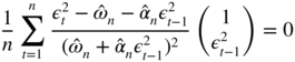
with, for instance . This estimator does not have an explicit form and must be obtained numerically. Theorem 7.2, which provides the asymptotic distribution of the estimator, only requires the extra assumption that θ ₀ belongs to . Thus, if α ₀ = 0 (that is, if the model is conditionally homoscedastic), the estimator remains consistent but is no longer asymptotically normal. Matrix J takes the form

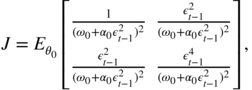
and the asymptotic variance of is

Table 7.1 displays numerical evaluations of this matrix. An estimation of J is obtained by replacing the expectations by empirical means, obtained from simulations of length 10 000, when η _t is 풩(0, 1) distributed. This experiment is repeated 1 000 times to obtain the results presented in the table.

images — Asymptotic variance for the QMLE of an ARCH(1) process with η _t∼풩(0, 1).

In order to assess, in finite samples, the quality of the asymptotic approximation of the variance of the estimator, the following Monte Carlo experiment is conducted. For the value θ ₀ of the parameter, and for a given length n , N samples are simulated, leading to N estimations of θ ₀ , i = 1, …, N . We denote by their empirical mean. The root mean squared error (RMSE) of estimation of α is denoted by

and can be compared to , the latter quantity being evaluated independently, by simulation. A similar comparison can obviously be made for the parameter ω . For θ ₀ = (0.2, 0.9)^′ and N = 1000, Table 7.2 displays the results, for different sample length n .

n		RMSE( α )
100	0.85221	0.25742	0.25014	0.266
250	0.88336	0.16355	0.15820	0.239
500	0.89266	0.10659	0.11186	0.152
1000	0.89804	0.08143	0.07911	0.100

The similarity between columns 3 and 4 is quite satisfactory, even for moderate sample sizes. The last column gives the empirical probability (that is, the relative frequency within the N samples) that is greater than 1 (which is the limiting value for second‐order stationarity). These results show that, even if the mean of the estimations is close to the true value for large n , the variability of the estimator remains high. Finally, note that the length n = 1000 remains realistic for financial series.

7.1.3 The Non‐stationary ARCH(1)

When the strict stationarity constraint is not satisfied in the ARCH(1) case, that is, when

7.14

one can define an ARCH(1) process starting with initial values. For a given value ε₀ , we define

7.15

where ω ₀ > 0 and α ₀ > 0, with the usual assumptions on the sequence (η _t). As already noted, converges to infinity almost surely when

7.16

and only in probability when the inequality (7.14) is an equality (see Corollary 2.1 and Remark 2.3 following it). Is it possible to estimate the coefficients of such a model? The answer is only partly positive: it is possible to consistently estimate the coefficient α ₀ , but the coefficient ω ₀ cannot be consistently estimated. The practical impact of this result thus appears to be limited, but because of its theoretical interest, the problem of estimating coefficients of non‐stationary models deserves attention. Consider the QMLE of an ARCH(1), that is to say a measurable solution of

7.17

where θ = (ω, α), Θ is a compact set of (0, ∞)² , and for t = 1, …, n (starting with a given initial value for ). The almost sure convergence of to infinity will be used to show the strong consistency of the QMLE of α ₀ . The following lemma completes Corollary 2.1 and gives the rate of convergence of to infinity under condition (7.16).

This result entails the strong consistency and asymptotic normality of the QMLE of α ₀ .

In the proof of this theorem, it is shown that the score vector satisfies

In the standard statistical inference framework, the variance J of the score vector is (proportional to) the Fisher information. According to the usual interpretation, the form of the matrix J shows that, asymptotically and for almost all observations, the variations of the log‐likelihood are insignificant when θ varies from (ω ₀, α ₀) to (ω ₀ + h, α ₀) for small h . In other words, the limiting log‐likelihood is flat at the point (ω ₀, α ₀) in the direction of variation of ω ₀ . Thus, minimising this limiting function does not allow θ ₀ to be found. This leads us to think that the QML of ω ₀ is likely to be inconsistent when the strict stationarity condition is not satisfied. Figure 7.2 displays numerical results illustrating the performance of the QMLE in finite samples. For different values of the parameters, 100 replications of the ARCH(1) model have been generated, for the sample sizes n = 200 and n = 4000. The top panels of the figure correspond to a second‐order stationary ARCH(1), with parameter θ ₀ = (1, 0.95). The panels in the middle correspond to a strictly stationary ARCH(1) of infinite variance, with θ ₀ = (1, 1.5). The results obtained for these two cases are similar, confirming that second‐order stationarity is not necessary for estimating an ARCH. The bottom panels, corresponding to the explosive ARCH(1) with parameter θ ₀ = (1, 4), confirm the asymptotic results concerning the estimation of α ₀ . They also illustrate the failure of the QML to estimate ω ₀ under the nonstationarity condition ( 7.16). The results even deteriorate when the sample size increases.

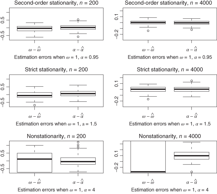
Image described by caption and surrounding text. — Figure 7.2 Box‐plots of the QML estimation errors for the parameters ω ₀ and α ₀ of an ARCH(1) process, with η _t∼풩(0, 1).

7.2 Estimation of ARMA–GARCH Models by Quasi‐Maximum Likelihood

In this section, the previous results are extended to cover the situation where the GARCH process is not directly observed, but constitutes the innovation of an observed ARMA process. This framework is relevant because, even for financial series, it is restrictive to assume that the observed series is the realisation of a noise. From a theoretical point of view, it will be seen that the extension to the ARMA–GARCH case is far from trivial. Assume that the observations X ₁, …, X _n are generated by a strictly stationary non‐anticipative solution of the ARMA(P, Q)‐GARCH(p, q) model

7.21

where (η _t) and the coefficients ω ₀ , α _0i and β _0j are defined as in model ( 7.1). The orders P, Q, p, q are assumed known. The vector of the parameters is denoted by

where θ is defined as in equality (7.2). The parameter space is

The true value of the parameter is denoted by

We still employ a Gaussian quasi‐likelihood conditional on initial values. If q ≥ Q , the initial values are

These values (the last p of which are positive) are assumed to be fixed, but they could depend on the parameter and/or on the observations. For any ϑ , the values of , for t = − q + Q + 1, …, n , and then, for any θ , the values of , for t = 1, …, n, can thus be computed from

7.22

When q < Q , the fixed initial values are

Conditionally on these initial values, the Gaussian log‐likelihood is given by

A QMLE is defined as a measurable solution of the equation

h3

Strong Consistency

Let and . Standard assumptions are made on these AR and MA polynomials, and assumption A1 is modified as follows:

A7: ϕ ₀ ∈ Φ and Φ is compact.
A8: For all ϕ ∈ Φ, a _ϑ(z)b _ϑ(z) = 0 implies ∣z ∣ > 1.
A9: and have no common roots, a _0P ≠ 0 or b _0Q ≠ 0.

Under assumptions A2 and A8, (X _t) is supposed to be the unique strictly stationary nonanticipative solution of model (7.21). Let and , where is the non‐anticipative and ergodic strictly stationary solution of ( 7.10). Note that e _t = ε_t(ϑ ₀) and . The following result is an extension of Theorem 7.1.

Asymptotic Normality When the Moment of Order 4 Exists

So far, the asymptotic results of the QMLE (consistency and asymptotic normality in the pure GARCH case, consistency in the ARMA–GARCH case) have not required any moment assumption on the observed process (for the asymptotic normality in the pure GARCH case, a moment of order 4 is assumed for the iid process, not for ε_t ). One might think that this will be the same for establishing the asymptotic normality in the ARMA–GARCH case. The following example shows that this is not the case.

Example 7.2 Non‐existence of J without moment assumption

Consider the AR(1)‐ARCH(1) model

7.23

where ∣a ₀₁ ∣ < 1, ω ₀ > 0, α ₀ ≥ 0, and the distribution of the iid sequence (η _t) is defined, for a > 1, by

Then the process (X _t) is always stationary, for any value of α ₀ (because ; see the strict stationarity constraint (2.10)). By contrast, X _t does not admit a moment of order 2 when α ₀ ≥ 1 (see Theorem 2.2). The first component of the (normalised) score vector is

We have

since, first, η _t − 1 = 0 entails ε_t − 1 = 0 and X _t − 1 = a ₀₁ X _t − 2 , and second, η _t − 1 and X _t − 2 are independent. Consequently, if and a ₀₁ ≠ 0, the score vector does not admit a variance.

This example shows that it is not possible to extend the result of asymptotic normality obtained in the GARCH case to the ARMA–GARCH models without additional moment assumptions. This is not surprising because for ARMA models (which can be viewed as limits of ARMA–GARCH models when the coefficients α _0i and β _0j tend to 0) the asymptotic normality of the QMLE is shown with second‐order moment assumptions. For an ARMA with infinite variance innovations, the consistency of the estimators may be faster than in the standard case and the asymptotic distribution belongs to the class of the α-stable laws, but is non‐Gaussian in general. We show the asymptotic normality with a moment assumption of order 4. Recall that, by Theorem 2.9, this assumption is equivalent to ρ{E(A _0t ⊗ A _0t)} < 1. We make the following assumptions:

A10 ρ{E(A _0t ⊗ A _0t)} < 1 and, for all θ ∈ Θ, .
A11 , where denotes the interior of Φ.
A12 There exists no set Λ of cardinality 2 such that ℙ(η _t ∈ Λ) = 1.

Assumption A10 implies that and makes assumption A2 superfluous. The identifiability assumption A12 is slightly stronger than the first part of assumption A3 when the distribution of η _t is not symmetric. We are now in a position to state conditions ensuring the asymptotic normality of the QMLE of an ARMA–GARCH model.

Remark 7.4

It is interesting to note that if η _t has a symmetric law, then the asymptotic variance Σ is block‐diagonal, which is interpreted as an asymptotic independence between the estimators of the ARMA coefficients and those of the GARCH coefficients. The asymptotic distribution of the estimators of the ARMA coefficients depends, however, on the GARCH coefficients (in view of the form of the matrices I ₁ and J ₁ involving the derivatives of ). On the other hand, still when the distribution of I and J is symmetric, the asymptotic accuracy of the estimation of the GARCH parameters is not affected by the ARMA part: the lower left block of Σ depends only on the GARCH coefficients. The block‐diagonal form of Σ may also be of interest for testing problems of joint assumptions on the ARMA and GARCH parameters.
Assumption A11 imposes the strict positivity of the GARCH coefficients and it is easy to see that this assumption constrains only the GARCH coefficients. For any value of ϑ ₀ , the restriction of Φ to its first P + Q + 1 coordinates can be chosen sufficiently large so that its interior contains ϑ ₀ and assumption A8 is satisfied.
In the proof of the theorem, the symmetry of the iid process distribution is used to show the following result, which is of independent interest.
7.24
provided this expectation exists (see Exercise 7.1).

Example 7.3 Numerical evaluation of the asymptotic variance

Consider the AR(1)‐ARCH(1) model defined by equation 7.23). In the case where η _t follows the 풩(0, 1) law, condition A10 for the existence of a moment of order 4 is written as , that is, α ₀ < 0.577 (see (2.54)). In the case where η _t follows the χ ²(1) distribution, normalised in such a way that Eη _t = 0 and , this condition is written as , that is, α ₀ < 0.258. To simplify the computation, assume that ω ₀ = 1 is known. Table 7.3 provides a numerical evaluation of the asymptotic variance Σ, for these two distributions and for different values of the parameters a ₀ and α ₀ . It is clear that the asymptotic variance of the two parameters strongly depends on the distribution of the iid process. These experiments confirm the independence of the asymptotic distributions of the AR and ARCH parameters in the case where the distribution of η _t is symmetric. They reveal that the independence does not hold when this assumption is relaxed. Note the strong impact of the ARCH coefficient on the asymptotic variance of the AR coefficient. On the other hand, the simulations confirm that in the case where the distribution is symmetric, the AR coefficient has no impact on the asymptotic accuracy of the ARCH coefficient. When the distribution is not symmetric, the impact, if there is any, is very weak. For the computation of the expectations involved in the matrix Σ, see Exercise 7.8. In particular, the values corresponding to α ₀ = 0 (AR(1) without ARCH effect) can be analytically computed. Note also that the results obtained for the asymptotic variance of the estimator of the ARCH coefficient in the case a ₀ = 0 do not coincide with those of Table 7.2. This is not surprising because in this table ω ₀ is not supposed to be known.

7.3 Application to Real Data

In this section, we employ the QML method to estimate GARCH(1, 1) models on daily returns of 11 stock market indices, namely the CAC, DAX, DJA, DJI, DJT, DJU, FTSE, Nasdaq, Nikkei, SMI, and S&P 500 indices. The observations cover the period from 2 January 1990 to 22 January 2009 ¹ (except for those indices for which the first observation is after 1990). The GARCH(1, 1) model has been chosen because it constitutes the reference model, by far the most commonly used in empirical studies. However, in Chapter 8, we will see that it can be worth considering models with higher orders p and q .

Table 7.4 displays the estimators of the parameters ω, α, β , together with their estimated standard deviations. The last column gives estimates of , obtained by replacing the unknown parameters by their estimates and by the empirical mean of the fourth‐order moment of the standardised residuals. We have if and only if ρ ₄ < 1. The estimates of the GARCH coefficients are quite homogenous over all the series and are similar to those usually obtained in empirical studies of daily returns. The coefficients α are close to 0.1, and the coefficients β are close to 0.9, which indicates a strong persistence of the shocks on the volatility. The sum α + β is greater than 0.98 for 10 of the 11 series, and greater than 0.96 for all the series. Since α + β < 1, the assumption of second‐order stationarity cannot be rejected, for any series (see Section 8.1). A fortiori, by Remark 2.6, the strict stationarity cannot be rejected. The existence of moments of order 4, , is questionable for all the series because is extremely close to 1. Recall, however, that consistency and asymptotic normality of the QMLE do not require any moment on the observed process but do require strict stationarity.

Index	ω	α	β	ρ ₄
CAC	0.033 (0.009)	0.090 (0.014)	0.893 (0.015)	1.0067
DAX	0.037 (0.014)	0.093 (0.023)	0.888 (0.024)	1.0622
DJA	0.019 (0.005)	0.088 (0.014)	0.894 (0.014)	0.9981
DJI	0.017 (0.004)	0.085 (0.013)	0.901 (0.013)	1.0020
DJT	0.040 (0.013)	0.089 (0.016)	0.894 (0.018)	1.0183
DJU	0.021 (0.005)	0.118 (0.016)	0.865 (0.014)	1.0152
FTSE	0.013 (0.004)	0.091 (0.014)	0.899 (0.014)	1.0228
Nasdaq	0.025 (0.006)	0.072 (0.009)	0.922 (0.009)	1.0021
Nikkei	0.053 (0.012)	0.100 (0.013)	0.880 (0.014)	0.9985
SMI	0.049 (0.014)	0.127 (0.028)	0.835 (0.029)	1.0672
S&P 500	0.014 (0.004)	0.084 (0.012)	0.905 (0.012)	1.0072

7.4 Proofs of the Asymptotic Results*

We denote by K > 0 and ρ ∈ [0, 1) generic constants whose values can vary from line to line. As an example, one can write for 0 < ρ ₁ < 1 and 0 < ρ ₂ < 1, i ₁ ≥ 0, i ₂ ≥ 0,

Proof of Theorem 7.1

Proof of Theorem 7.1

The proof is based on a vectorial autoregressive representation of order 1 of the vector , analogous to that used for the study of stationarity. Assumption A2 allows us to write as a series depending on the infinite past of the variable . It can be shown that the initial values are not important asymptotically, using the fact that, under the strict stationarity assumption, necessarily admits a moment order s , with s > 0. This property also allows us to show that the expectation of ℓ_t(θ ₀) is well defined in ℝ and that , which guarantees that the limit criterion is minimised at the true value. The difficulty is that can be equal to +∞. Assumptions A3 and A4 are crucial to establishing the identifiability: the former assumption precludes the existence of a constant linear combination of , j ≥ 0. The assumption of absence of common root is also used. The ergodicity of ℓ_t(θ) and a compactness argument conclude the proof.

It will be convenient to rewrite equation 7.10) in matrix form. We have

7.25

where

7.26

We will establish the following intermediate results.

(a) , a.s..
(b) .
(c) , and if θ ≠ θ ₀ , .
(d)For any θ ≠ θ ₀ , there exists a neighbourhood V(θ) such that

(a) Asymptotic irrelevance of the initial values
In view of Corollary 2.2, the condition of assumption A2 implies that ρ(B) < 1. The compactness of Θ implies that

7.27

Iterating (7.25), we thus obtain

7.28

Let be the vector obtained by replacing by in , and let be the vector obtained by replacing by the initial values ( 7.6) or ( 7.7). We have

7.29

From inequality (7.27), it follows that almost surely

7.30

For x > 0 we have log x ≤ x − 1. It follows that, for x, y > 0, . We thus have almost surely, using inequality (7.30),

7.31

The existence of a moment of order s > 0 for , deduced from assumption A1 and Corollary 2.3, allows us to show that a.s. (see Exercise 7.2). Using Cesàro's lemma, point (a) follows.
(b) Identifiability of the parameter
Assume that , almost surely. By Corollary 2.2, the polynomial ℬ _θ(B) is invertible under assumption A2. Using equality ( 7.10), we obtain

If the operator in B between braces were not null, then there would exist a constant linear combination of the , j ≥ 0. Thus the linear innovation of the process would be equal to zero. Since the distribution of is non‐degenerate, in view of assumption A3,

We thus have

7.32

Under assumption A4 (absence of common root), it follows that , and ω = ω ₀ . We have thus shown (b).
(c) The limit criterion is minimised at the true value
The limit criterion may not be integrable at some points, but is well defined in ℝ ∪ {+∞} because, with the notation x ⁻ = max(−x, 0) and x ⁺ = max(x, 0), ²

It is, however, possible to have for some values of θ . This occurs, for instance when θ = (ω, 0, …, 0) and (ε_t) is an IGARCH such that . We will see that this cannot occur at θ ₀ , meaning that the limit criterion is integrable at θ ₀ . To establish this result, we have to show that . Using Jensen's inequality and, once again, the existence of a moment of order s > 0 for , we obtain

because

Thus

Having already established that , it follows that is well defined in ℝ. Since for all x > 0, log x ≤ x − 1 with equality if and only if x = 1, we have

7.33

with equality if and only if ‐a.s., that is, in view of (b), if and only if θ = θ ₀ . ³
(d) Compactness of Θ and ergodicity of (ℓ_t(θ))
For all θ ∈ Θ and any positive integer k , let V _k(θ) be the open ball of centre θ and radius 1/k . Because of (a), we have

To obtain the convergence of this empirical mean, the standard ergodic theorem cannot be applied (see Theorem A.2) because we have seen that ℓ_t(θ ^*) is not necessarily integrable, except at θ ₀ . We thus use a modified version of this theorem, which allows for an ergodic and strictly stationary sequence of variables admitting an expectation in ℝ ∪ {+∞} (see Exercise 7.3). This version of the ergodic theorem can be applied to {ℓ_t(θ ^*)}, and thus to (see Exercise 7.4), which allows us to conclude that

By Beppo Levi's theorem, increases to as k → ∞. Given relation (7.33), we have shown (d).

The conclusion of the proof uses a compactness argument. First note that for any neighbourhood V(θ ₀) of θ ₀ ,

7.34

The compact set Θ is covered by the union of an arbitrary neighbourhood V(θ ₀) of θ ₀ and the set of the neighbourhoods V(θ) satisfying (d), θ ∈ ΘV(θ ₀). Thus, there exists a finite subcover of Θ of the form V(θ ₀), V(θ ₁), …, V(θ _k), where, for i = 1, …, k , V(θ _i) satisfies (d). It follows that

The relations (d) and (7.34) show that, almost surely, belongs to V(θ ₀) for n large enough. Since this is true for any neighbourhood V(θ ₀), the proof is complete.

Proof of Theorem 7.2

Proof of Theorem 7.2

The proof of this theorem is based on a standard Taylor expansion of criterion (7.8) at θ ₀ . Since converges to θ ₀ , which lies in the interior of the parameter space by assumption A5, the derivative of the criterion is equal to zero at . We thus have

7.35

where the are between and θ ₀ . It will be shown that

7.36

and that

7.37

The proof of the theorem immediately follows. We will split the proof of convergences (7.36) and (7.37) into several parts:

(a) , .
(b) J is invertible and .
(c)There exists a neighbourhood 풱(θ ₀) of θ ₀ such that, for all i, j, k ∈ {1, …, p + q + 1},
(d) and tend in probability to 0 as n → ∞.
(e) .
(f) a.s.
(a) Integrability of the derivatives of the criterion at θ ₀ .
Since , we have

7.38

7.39

At θ = θ ₀ , the variable is independent of and its derivatives. To show (a), it thus suffices to show that

7.40

In view of relation (7.28), we have

7.41

7.42

where , , and B ^(j) is a p × p matrix with 1 in position (1, j) and zeros elsewhere. Note that, in view of the positivity of the coefficients and relations (7.41) and (7.42), the derivatives of are positive or null. In view of relations ( 7.41), it is clear that is bounded. Since , the variable is also bounded. This variable thus possesses moments of all orders. In view of the second equality in relations ( 7.41) and of the positivity of all the terms involved in the sums, we have

It follows that

7.43

The variable thus admits moments of all orders at θ = θ ₀ . In view of ( 7.42) and β _j B ^(j) ≤ B , we have

7.44

Using inequality ( 7.27), we have ‖B ^k‖ ≤ Kρ ^k for all k . Moreover, having a moment of order s ∈ (0, 1), the variable has the same moment. ⁴ Using in addition (7.44), the inequality and the relation x/(1 + x) ≤ x ^s for all x ≥ 0, ⁵ we obtain

7.45

Under assumption A5 we have β _0j > 0 for all j , which entails that the first expectation in (7.40) exists.

We now turn to the higher‐order derivatives of . In view of the first equality of relations ( 7.41), we have

7.46

We thus have

which is a vector of finite constants (since ρ(B) < 1). It follows that is bounded, and thus admits moments of all orders. It is of course the same for . The second equality of ( 7.41) gives

7.47

The arguments used to show the inequality (7.45) then show that

This entails that is integrable. Differentiating relation ( 7.42) with respect to , we obtain

7.48

because β _j B ^(j) ≤ B . As for ( 7.45), it follows that

and the existence of the second expectation in ( 7.40) is proven.

Since is bounded, and since by inequality (7.43) the variables are bounded at θ ₀ , it is clear that

for i = 1, …, q + 1. With the notation and arguments already used to show ( 7.45), and using the elementary inequality x/(1 + x) ≤ x ^s/2 for all x ≥ 0, Minkowski's inequality implies that

Finally, the Cauchy–Schwarz inequality entails that the third expectation of ( 7.40) exists.
(b) Invertibility of J and connection with the variance of the criterion derivative.
Using (a), and once again, the independence between and and its derivatives, we have by relation (7.38),

Moreover, in view of the moment conditions ( 7.40), J exists and satisfies relation (7.13). We also have

7.49

Assume now that J is singular. Then there exists a non‐zero vector λ in ℝ^{p + q + 1} such that a.s. ⁶ In view of relation ( 7.10) and the stationarity of , we have

Let λ = (λ ₀, λ ₁, …, λ _q + p)^′ . It is clear that λ ₁ = 0, otherwise would be measurable with respect to the σ ‐field generated by {η _u, u < t − 1}. For the same reason, we have λ ₂ = ⋯ = λ _2 + i = 0 if λ _q + 1 = ⋯ = λ _q + i = 0. Consequently, λ ≠ 0 implies the existence of a GARCH(p − 1, q − 1) representation. By the arguments used to show relations (7.32), assumption A4 entails that this is impossible. It follows that λ ^′ Jλ = 0 implies λ = 0, which completes the proof of (b).
(c) Uniform integrability of the third‐order derivatives of the criterion.
Differentiating relation (7.39), we obtain

7.50

We begin by studying the integrability of . This is the most difficult term to deal with. Indeed, the variable is not uniformly integrable on Θ: at θ = (ω, 0^′), the ratio is integrable only if exists. We will, however, show the integrability of uniformly in θ in the neighbourhood of θ ₀ . Let Θ^* be a compact set which contains θ ₀ and which is contained in the interior of Θ (∀θ ∈ Θ^* , we have θ ≥ θ _* > 0 component by component). Let B ₀ be the matrix B (defined in (7.26)) evaluated at the point θ = θ ₀ . For all δ > 0, there exists a neighbourhood 풱(θ ₀) of θ ₀ , included in Θ^* , such that for all θ ∈ 풱(θ ₀),

Note that, since 풱(θ ₀) ⊂ Θ^* , we have From relation ( 7.28), we obtain

and, again using x/(1 + x) ≤ x ^s for all x ≥ 0 and all s ∈ (0, 1),

7.51

If s is chosen such that and, for instance, δ = (1 − ρ ^s)/(2ρ ^s), then the expectation of the previous series is finite. It follows that there exists a neighbourhood 풱(θ ₀) of θ ₀ such that

Using inequality (7.51), keeping the same choice of δ but taking s such that , the triangle inequality gives

7.52

Now consider the second term in braces in the right‐hand side of equality (7.50). Differentiating relations (7.46), (7.47), and (7.48), with the arguments used to show inequality ( 7.43), we obtain

when the indices i ₁ , i ₂ and i ₃ are not all in {q + 1, q + 2, …, q + 1 + p} (that is, when the derivative is taken with respect to at least one parameter different from the β _j ). Using again the arguments used to show relations ( 7.44) and ( 7.48), and then inequality ( 7.45), we obtain

for any s ∈ (0, 1). Since for some s > 0, it follows that

7.53

It is easy to see that in this inequality the power 2 can be replaced by any power d :

Using the Cauchy–Schwarz inequality, and the moment conditions (7.52) and (7.53), we obtain

The other terms in braces in the right‐hand side of equality ( 7.50) are handled similarly. We show in particular that

7.54

for any integer d . With the aid of Hölder's inequality, this allows us to establish, in particular, that

Thus we obtain (c).

(d) Asymptotic decrease of the effect of the initial values.
Using relation (7.29), we obtain the analogs of ( 7.41) and ( 7.42) for the derivatives of :

7.55

7.56

7.57

where is equal to (0, …, 0)^′ when the initial conditions are given by ( 7.7), and is equal to (1, …, 1)^′ when the initial conditions are given by ( 7.6). The second‐order derivatives have similar expressions. The compactness of Θ and the fact that ρ(B) < 1 allow us to claim that, almost surely,

7.58

Using ( 7.30), we obtain

7.59

Since

we have, using inequalities (7.59) and the first inequality in (7.58),

It follows that

7.60

Markov's inequality, ( 7.40), and the independence between η _t and imply that, for all ε > 0,

which, by inequality (7.60), shows the first part of (d).

Now consider the asymptotic impact of the initial values on the second‐order derivatives of the criterion in a neighbourhood of θ ₀ . In view of ( 7.39) and the previous computations, we have

where

In view of ( 7.52), (7.54), and Hölder's inequality, it can be seen that, for a certain neighbourhood 풱(θ ₀), the expectation of ϒ_t is a finite constant. Using Markov's inequality once again, the second convergence of (d) is then shown.
(e) CLT for martingale increments.
The conditional score vector is obviously centred, which can be seen from equality ( 7.38), using the fact that and its derivatives belong to the σ ‐field generated by {ε_t − i, i ≥ 0}, and the fact that :

Note also that by relation (7.49), is finite. In view of the invertibility of J and the assumptions on the distribution of η _t (which entail 0 < κ _η − 1 < ∞), this covariance matrix is non‐degenerate. It follows that, for all λ ∈ ℝ^{p + q + 1} , the sequence is a square integrable ergodic stationary martingale difference. Corollary A.1 and the Cramér–Wold theorem (see, for example, Billingsley 1995, pp. 383, 476 and 360) entail (e).
(f) Use of a second Taylor expansion and of the ergodic theorem.
Consider the Taylor expansion (7.35) of the criterion at θ ₀ . We have, for all i and j ,

7.61

where is between and θ ₀ . The almost sure convergence of to θ ₀ , the ergodic theorem and (c) imply that almost surely

Since almost surely, the second term on the right‐hand side of equality (7.61) converges to 0 with probability 1. By the ergodic theorem, the first term on the right‐hand side of equality ( 7.61) converges to J(i, j). To complete the proof of Theorem 7.2, it suffices to apply Slutsky's lemma. In view of (d), (e) and (f) we obtain convergences ( 7.36) and ( 7.37).

To prove the asymptotic normality of the QMLE, we need the following intermediate result.

Proof of (7.20)

Proof of ( 7.20)

We remark that we do not know, a priori, if the derivative of the criterion is equal to zero at , because we only have the convergence of to α ₀ . Thus the minimum of the criterion could lie at the boundary of Θ, even asymptotically. By contrast, the partial derivative with respect to the second coordinate must asymptotically vanish at the optimum, since and . A Taylor expansion of the derivative of the criterion thus gives

7.67

where J _n is a 2 × 2 matrix whose elements are of the form

with between and θ ₀ . By Lemma 7.1, which shows that almost surely, and by the central limit theorem of Lindeberg for martingale increment (see Corollary A.1),

7.68

Relation ( 7.64) of Lemma 7.2 and the compactness of Θ show that

7.69

By a Taylor expansion of the function

we obtain

where α ^* is between and α ₀ . Using results ( 7.65), ( 7.66), and ( 7.19), we obtain

7.70

We conclude using the second row of (7.67), and also using (7.68), (7.69), and (7.70).

Proof of Theorem 7.4

Proof of Theorem 7.4

The proof follows the steps of the proof of Theorem 7.1. We will show the following points:

(a) , a.s.
(b) .
(c)If ϕ ≠ ϕ ₀ , .
(d)For any ϕ ≠ ϕ ₀ there exists a neighbourhood V(ϕ) such that

(a) Nullity of the asymptotic impact of the initial values.
Equations ( 7.10)–( 7.28) remain valid under the convention that ε_t = ε_t(ϑ). Equation ( 7.29) must be replaced by

7.71

where , the ‘tilde’ variables being initialised as indicated before. Assumptions A7 and A8 imply that,

7.72

It follows that almost surely

and thus, by relations ( 7.28), (7.71) and ( 7.27),

7.73

Similarly, we have that almost surely . The difference between the theoretical log‐likelihoods with and without initial values can thus be bounded as follows:

This inequality is analogous to inequality (7.31), being replaced by . Following the lines of the proof of (a) in Theorem 7.1 (see Exercise 7.2), it suffices to show that for all real r > 0, E(ρ ^t ξ _t)^r is the general term of a finite series. Note that ⁷

since, by Corollary 2.3, Statement (a) follows.
(b) Identifiability of the parameter.
If ε_t(ϑ) = ε_t(ϑ ₀) almost surely, assumptions A8 and A9 imply that there exists a constant linear combination of the variables X _t − j , j ≥ 0. The linear innovation of (X _t), equal to X _t − E(X _t ∣ X _u, u < t) = η _t σ _t(ϕ ₀), is zero almost surely only if η _t = 0 a.s. (since ). This is precluded, since . It follows that ϑ = ϑ ₀ , and thus that θ = θ ₀ by the argument used in the proof of Theorem 7.1.
(c) The limit criterion is minimised at the true value.
By the arguments used in the proof of (c) in Theorem 7.1, it can be shown that, for all ϕ , is defined in ℝ ∪ {+∞}, and in ℝ at ϕ = ϕ ₀ . We have

because the last expectation is equal to 0 (noting that ε_t(ϑ) − ε_t(ϑ ₀) belongs to the past, as well as σ _t(ϕ ₀) and σ _t(ϕ)), the other expectations being positive or null by arguments already used. This inequality is strict only if ε_t(ϑ) = ε_t(ϑ ₀) and if a.s. which, by (b), implies ϕ = ϕ ₀ and completes the proof of (c).
(d) Use of the compactness of Φ and of the ergodicity of (ℓ_t(ϕ)).
The end of the proof is the same as that of Theorem 7.1.

Proof of Theorem 7.5

Proof of Theorem 7.5

The proof follows the steps of that of Theorem 7.2. The block‐diagonal form of the matrices when the distribution of η _t is symmetric is shown in Exercise 7.7. It suffices to establish the following properties.

(a) , .
(b)ℐ and are invertible.
(c) and tend in probability to 0 as n → ∞.
(d) .
(e) a.s., for all ϕ ^* between and ϕ ₀ .

Formulas ( 7.38) and ( 7.39) giving the derivatives with respect to the GARCH parameters (that is, the vector θ ) remain valid in the presence of an ARMA part (writing ). The same is true for all the results established in (a) and (b) of the proof of Theorem 7.2, with obvious changes of notation. The derivatives of with respect to the parameter ϑ , and the cross derivatives with respect to θ and ϑ , are given by

7.74

The derivatives of ε_t are of the form

where

7.77

and

7.78

where H _{k, ℓ}(t) is the k × ℓ (Hankel) matrix of general term ε_{t − i − j} , and 0_{k, ℓ} denotes the null matrix of size k × ℓ. Moreover, by relation ( 7.28),

7.79

where ϑ _j denotes the j th component of ϑ , and

7.80

(a) Integrability of the derivatives of the criterion at φ ₀ .
The existence of the expectations in ( 7.40) remains true. By (7.74)–(7.76), the independence between (ε_t/σ _t)(ϕ ₀) = η _t and , its derivatives, and the derivatives of ε_t(ϑ ₀), using and , it suffices to show that

7.81

7.82

to establish point (a), together with the existence of the matrices ℐ and . By the expressions for the derivatives of ε_t , (7.77)–(7.78), and using , we obtain the moment conditions (7.81).

The Cauchy–Schwarz inequality implies that

Thus, in view of relation (7.79) and the positivity of ω ₀ ,

Using the triangle inequality and the elementary inequalities (∑ ∣ x _i∣)^1/2 ≤ ∑ |x _i|^1/2 and x/(1 + x ²) ≤ 1, it follows that

7.83

The first inequality of (7.82) follows. The existence of the second expectation in ( 7.82) is a consequence of (7.80), the Cauchy–Schwarz inequality, and the square integrability of ε_t and its derivatives. To handle the second‐order partial derivatives of , first note that by ( 7.41). Moreover, using relation ( 7.79),

7.84

By the arguments used to show inequality ( 7.44), we obtain

7.85

which entails the existence of the third expectation in ( 7.82).
(b) Invertibility of ℐ and .
Assume that ℐ is non‐invertible. There exists a non‐zero vector λ in ℝ^{P + Q + p + q + 2} such that λ ^′ ∂ℓ_t(ϕ ₀)/∂ϕ ^′ = 0 a.s. By relations ( 7.38) and ( 7.74), this implies that

7.86

Taking the variance of the left‐hand side, conditionally on the σ ‐field generated by {η _u, u < t}, we obtain a.s., at ϕ = ϕ ₀ ,

where . It follows that and almost surely. By stationarity, we have either for all t , or for all t . Consider for instance the latter case, the first one being treated similarly. Relation (7.86) implies . The term in brackets cannot vanish almost surely, otherwise η _t would take at least two different values, which would be in contradiction to assumption A12. It follows that a _t = 0 a.s. and thus b _t = 0 a.s. We have shown that almost surely

7.87

where λ ₁ is the vector of the first P + Q + 1 components of λ . By stationarity of (∂ε_t/∂ϕ)_t , the first equality implies that

We now use assumption A9, that the ARMA representation is minimal, to conclude that λ ₁ = 0. The third equality in (7.87) is then written, with obvious notation, as . We have already shown in the proof of Theorem 7.2 that this entails λ ₂ = 0. We are led to a contradiction, which proves that ℐ is invertible. Using relations ( 7.39) and (7.75)–( 7.76), we obtain

We have just shown that the first expectation is a positive definite matrix. The second expectation being a positive semidefinite matrix, is positive definite and thus invertible, which completes the proof of (b).
(c) Asymptotic unimportance of the initial values.
The initial values being fixed, the derivatives of , obtained from ( 7.71), are given by

with the notation introduced in relations ( 7.41)–( 7.42) and (7.55)–(7.56). As for relation ( 7.79), we obtain

and, by an obvious extension of inequality (7.72),

7.88

Thus

The latter sum converges almost surely because its expectation is finite. We have thus shown that

The other derivatives of are handled similarly, and we obtain

We have, in view of inequality (7.73),

where It is also easy to check that for ϕ = ϕ ₀ ,

It follows that, using the inequality (7.88),

Using the independence between η _t and S _t − 1 , ( 7.40), (7.83), the Cauchy–Schwarz inequality and , we obtain

which shows the first part of (c). The second is established by the same arguments.
(d) Use of a CLT for martingale increments.
The proof of this point is exactly the same as that of the pure GARCH case (see the proof of Theorem 7.2).
(e) Convergence to the matrix .
This part of the proof differs drastically from that of Theorem 7.2. For pure GARCH, we used a Taylor expansion of the second‐order derivatives of the criterion, and showed that the third‐order derivatives were uniformly integrable in a neighbourhood of θ ₀ . Without additional assumptions, this argument fails in the ARMA–GARCH case because variables of the form do not necessarily have moments of all orders, even at the true value of the parameter. First note that, since exists, the ergodic theorem implies that

The consistency of having already been established, and it suffices to show that for all ε > 0, there exists a neighbourhood 풱(ϕ ₀) of ϕ ₀ such that almost surely

7.89

(see Exercise 7.9). We first show that there exists 풱(ϕ ₀) such that

7.90

By Hölder's inequality, relations ( 7.39), ( 7.75), and ( 7.76), it suffices to show that for any neighbourhood 풱(ϕ ₀) ⊂ Φ whose elements have their components α _i and β _j bounded above by a positive constant, the quantities

7.91

7.92

7.93

are finite. Using the expansion of the series

similar expansions for the derivatives, and ‖ε_t(ϑ ₀)‖₄ < ∞ , it can be seen that the norms in (7.91) are finite. In (7.92), the first norm is finite, as an obvious consequence of , this latter term being strictly positive by compactness of Φ. An extension of inequality ( 7.83) leads to

Moreover, since relations ( 7.41)–( 7.44) remain valid when ε_t is replaced by ε_t(ϑ), it can be shown that

for any d > 0 and any neighbourhood 풱(ϕ ₀) whose elements have their components α _i and β _j bounded from below by a positive constant. The norms in ( 7.92) are thus finite. The existence of the first norm of (7.93) follows from ( 7.80) and ( 7.91). To handle the second one, we use (7.84), (7.85), ( 7.91), and the fact that . Finally, it can be shown that the third norm is finite by ( 7.47), ( 7.48) and by arguments already used. The property (7.90) is thus established. The ergodic theorem shows that the limit in (7.89) is equal almost surely to

By the dominated convergence theorem, using ( 7.90), this expectation tends to 0 when the neighbourhood 풱(ϕ ₀) tends to the singleton {ϕ ₀}. Thus ( 7.89) hold true, which proves (e). The proof of Theorem 7.5 is now complete.

7.5 Bibliographical Notes

The asymptotic properties of the QMLE of the ARCH models have been established by Weiss (1986) under the condition that the moment of order 4 exists. In the GARCH(1, 1) case, the asymptotic properties have been established by Lumsdaine (1996) (see also Lee and Hansen 1994) for the local QMLE under the strict stationarity assumption. In Lumsdaine (1996), the conditions on the coefficients α ₁ and β ₁ allow to handle the IGARCH(1, 1) model. They are, however, very restrictive with regard to the iid process: it is assumed that E|η _t|³² < ∞ and that the density of η _t has a unique mode and is bounded in a neighbourhood of 0. In Lee and Hansen (1994), the consistency of the global estimator is obtained under the assumption of second‐order stationarity.

Berkes, Horváth, and Kokoszka (2003b) was the first paper to give a rigorous proof of the asymptotic properties of the QMLE in the GARCH(p, q) case under very weak assumptions; see also Berkes and Horváth (2003b, 2004), together with Boussama (1998, 2000). The assumptions given in Berkes, Horváth, and Kokoszka (2003b) were weakened slightly in Francq and Zakoïan (2004). The proofs presented here come from that paper. An extension to non‐iid errors was proposed by Escanciano (2009).

Jensen and Rahbek (2004a,b) have shown that the parameter α ₀ of an ARCH(1) model, or the parameters α ₀ and β ₀ of a GARCH(1, 1) model, can be consistently estimated, with a standard Gaussian asymptotic distribution and a standard rate of convergence, even if the parameters are outside the strict stationarity region. They considered a constrained version of the QMLE, in which the intercept ω is fixed (see Exercises 7.13 and 7.14). These results were misunderstood by a number of researchers and practitioners, who wrongly claimed that the QMLE of the GARCH parameters is consistent and asymptotically normal without any stationarity constraint. We have seen in Section 3.1.3 that the QMLE of ω ₀ is inconsistent in the non‐stationary ARCH(1) case. The asymptotic properties of the unconstrained QMLE for non‐stationary GARCH(1,1)‐type models were studied in Francq and Zakoian (, 2013b), as well as tests of strict stationarity and non‐stationarity.

For ARMA–GARCH models, asymptotic results have been established by Ling and Li (1997, 1998), Ling and McAleer (2003a,b), and Francq and Zakoïan (2004). A comparison of the assumptions used in these papers can be found in the last reference. We refer the reader to Straumann (2005) for a detailed monograph on the estimation of GARCH models, to Francq and Zakoïan (2009a) for a review of the literature, and to Straumann and Mikosch (2006) and Bardet and Wintenberger (2009) for extensions to other conditionally heteroscedastic models. Li, Ling, and McAleer (2002) reviewed the literature on the estimation of ARMA–GARCH models, including in particular the case of nonstationary models.

The proof of the asymptotic normality of the QMLE of ARMA models under the second‐order moment assumption can be found, for instance, in Brockwell and Davis (1991). For ARMA models with infinite variance noise, see Davis, Knight, and Liu (1992), Mikosch et al. (1995), and Kokoszka and Taqqu (1996).

7.6 Exercises

7.1 (The distribution of η _t is symmetric for GARCH models)
The aim of this exercise is to show property (7.24).
1. Show the result for j < 0.
2. For j ≥ 0, explain why can be written as for some function h .
3. Complete the proof of ( 7.24).
7.2 (Almost sure convergence to zero at an exponential rate)
Let (ε_t) be a strictly stationary process admitting a moment order s > 0. Show that if ρ ∈ (0, 1), then a.s.
7.3 (Ergodic theorem for nonintegrable processes)
Prove the following ergodic theorem. If (X _t) is an ergodic and strictly stationary process and if EX ₁ exists in ℝ ∪ {+∞}, then

The result is shown in Billingsley (1995, p. 284) for iid variables.

Hint: Consider the truncated variables where κ > 0 with κ tending to +∞.
7.4 (Uniform ergodic theorem)
Let {X _t(θ)} be a process of the form

7.94

where (η _t) is strictly stationary and ergodic and f is continuous in θ ∈ Θ, Θ being a compact subset of ℝ^d .
1. Show that the process is strictly stationary and ergodic.
2. Does the property still hold true if X _t(θ) is not of the form (7.94), but it is assumed that {X _t(θ)} is strictly stationary and ergodic and that X _t(θ) is a continuous function of θ ?
7.5 (OLS estimator of a GARCH)
In the framework of the GARCH(p, q) model (7.1), an OLS estimator of θ is defined as any measurable solution of

where

and is defined by (7.4) with, for instance, initial values given by (7.6) or (7.7). Note that the estimator is unconstrained and that the variable can take negative values. Similarly, a constrained OLS estimator is defined by

The aim of this exercise is to show that under the assumptions of Theorem 7.1, and if , the constrained and unconstrained OLS estimators are strongly consistent. We consider the theoretical criterion
1. Show that almost surely as n → ∞ .
2. Show that the asymptotic criterion is minimised at θ ₀ ,
  
  and that θ ₀ is the unique minimum.
3. Prove that almost surely as n → ∞.
4. Show that almost surely as n → ∞.
7.6 (The mean of the squares of the normalised residuals is equal to 1)
For a GARCH model, estimated by QML with initial values set to zero, the normalized residuals are defined by , t = 1, …, n . Show that almost surely, for Θ large enough,

Hint: Note that for all c > 0 and all θ ∈ Θ, there exists such that for all t ≥ 0, and consider the function .
7.7 ( block‐diagonal)
Show that have the block‐diagonal form given in Theorem 7.5 when the distribution of η _t is symmetric.
7.8 (Forms of ℐ and in the AR(1)‐ARCH(1) case)
We consider the QML estimation of the AR(1)‐ARCH(1) model

assuming that ω ₀ = 1 is known and without specifying the distribution of η _t .
1. Give the explicit form of the matrices in Theorem 7.5 (with an obvious adaptation of the notation because the parameter here is (a ₀, α ₀)).
2. Give the block‐diagonal form of these matrices when the distribution of η _t is symmetric, and verify that the asymptotic variance of the estimator of the ARCH parameter
  1. does not depend on the AR parameter, and
  2. is the same as for the estimator of a pure ARCH (without the AR part).
3. Compute Σ when α ₀ = 0. Is the asymptotic variance of the estimator of a ₀ the same as that obtained when estimating an AR(1)? Verify the results obtained by simulation in the corresponding column of Table 7.3.
7.9 (A useful result in showing asymptotic normality)
Let (J _t(θ)) be a sequence of random matrices, which are function of a vector of parameters θ . We consider an estimator which strongly converges to the vector θ ₀ . Assume that

where J is a matrix. Show that if for all ε > 0 there exists a neighbourhood V(θ ₀) of θ ₀ such that

7.95

where ‖ ⋅ ‖ denotes a matrix norm, then

Give an example showing that condition (7.95) is not necessary for the latter convergence to hold in probability.
7.10 (A lower bound for the asymptotic variance of the QMLE of an ARCH)
Show that, for the ARCH( q ) model, under the assumptions of Theorem 7.2,

in the sense that the difference is a positive semi‐definite matrix.

Hint: Compute and show that is a variance matrix.
7.11 (A striking property of )
For a GARCH(p, q) model we have, under the assumptions of Theorem 7.2,

The objective of the exercise is to show that

7.96
1. Show the property in the ARCH case.
  Hint: Compute , and .
2. In the GARCH case, let . Show that
3. Complete the proof of (7.96).
7.12 (A condition required for the generalised Bartlett formula)
Using (7.24), show that if the distribution of η _t is symmetric and if , then formula (B.13) holds true, that is,
7.13 (Constrained QMLE of the parameter α ₀ of a nonstationary ARCH(1) process)
Jensen and Rahbek (2004a) consider the ARCH(1) model (7.15), in which the parameter ω ₀ > 0 is assumed to be known ( ω ₀ = 1 for instance) and where only α ₀ is unknown. They work with the constrained QMLE of α ₀ defined by

7.97

where . Assume therefore that ω ₀ = 1 and suppose that the nonstationarity condition (7.16) is satisfied.
1. Verify that
  
  and that
2. Prove that
3. Determine the almost sure limit of
4. Show that for all , almost surely
5. Prove that if almost surely (see Exercise 7.14) then
6. Does the result change when and ω ₀ ≠ 1?
7. Discuss the practical usefulness of this result for estimating ARCH models.
7.14 (Strong consistency of Jensen and Rahbek's estimator)
We consider the framework of Exercise 7.13, and follow the lines of the proof of (7.19)
1. Show that converges almost surely to α ₀ when ω ₀ = 1.
2. Does the result change if is replaced by and if ω and ω ₀ are arbitrary positive numbers? Does it entail the convergence result (7.19)?

Notes

..................Content has been hidden....................

You can't read the all page of ebook, please click here login for view all page.

	α ₀ = 0	α ₀ = 0.1	α ₀ = 0.25	x ∈ [0, 1]
a ₀ = 0
η _t ∼ 풩(0, 1)
η _t∼χ ²(1)				–
a ₀ = − 0.5
η _t∼풩(0, 1)
η _t∼χ ²(1)				–
a ₀ = − 0.9
η _t∼풩(0, 1)
η _t∼χ ²(1)				–

Table of Contents for 7 Estimating GARCH Models by Quasi‐Maximum Likelihood

Create new playlist

Sign In

Sign Up

7.1 Conditional Quasi‐Likelihood

h3

Likelihood Equations

7.1.1 Asymptotic Properties of the QMLE

Strong Consistency

Asymptotic Normality

7.1.2 The ARCH(1) Case: Numerical Evaluation of the Asymptotic Variance

7.1.3 The Non‐stationary ARCH(1)

7.2 Estimation of ARMA–GARCH Models by Quasi‐Maximum Likelihood

h3

Strong Consistency

Asymptotic Normality When the Moment of Order 4 Exists

7.3 Application to Real Data

7.4 Proofs of the Asymptotic Results*

7.5 Bibliographical Notes

7.6 Exercises

Notes

Table of Contents for
7 Estimating GARCH Models by Quasi‐Maximum Likelihood