Appendix E
Solutions to the Exercises
Chapter 1
- 1.1
-
- (a) We have the stationary solution X t = ∑ i ≥ 00.5 i (η t − i + 1), with mean EX t = 2 and autocorrelations ρ X (h) = 0.5∣h∣ .
- (b) We have an ‘anticipative’ stationary solutionwhich is such that EX t = − 1 and ρ X (h) = 0.5∣h∣ .

- (c) The stationary solutionis such that EX t = 2 with ρ X (1) = 2/19 and ρ X (h) = 0.5 h − 1 ρ X (1) for h > 1.

- The compatible models are, respectively, ARMA(1, 2), MA(3) and ARMA(1, 1).
- The first noise is strong, and the second is weak because

Note that, by Jensen's inequality, this correlation is positive.
-
- 1.2 Without loss of generality, assume
 for
t < 1 or
t > n
. We have
for
t < 1 or
t > n
. We have
which gives
 , and the result follows.
 - 1.3 Consider the degenerate sequence (X
t
)
t = 0, 1, …
defined, on a probability space (Ω, 풜, ℙ), by
X
t
(ω) = (−1)
t
for all
ω ∈ Ω and all
t ≥ 0. With probability 1, the sequence {(−1)
t
} is the realisation of the process (X
t
). This process is non‐stationary because, for instance,
EX
0 ≠ EX
1
.
Let U be a random variable, uniformly distributed on {0, 1}. We define the process (Y t ) t = 0, 1, … by

for any ω ∈ Ω and any t ≥ 0. The process (Y t ) is stationary. We have in particular EY t = 0 and Cov(Y t , Y t + h ) = (−1) h . With probability 1/2, the realisation of the stationary process (Y t ) will be the sequence {(−1) t } (and with probability 1/2, it will be {(−1) t + 1}).
This example leads us to think that it is virtually impossible to determine whether a process is stationary or not, from the observation of only one trajectory, even of infinite length. However, practitioners do not consider {(−1) t } as a potential realisation of the stationary process (Y t ). It is more natural, and simpler, to suppose that {(−1) t } is generated by the non‐stationary process (X t ).
- 1.4 The sequence 0, 1, 0, 1, … is a realisation of the process
X
t
= 0.5(1 + (−1)
t
A), where
A
is a random variable such that
P[A = 1] = P[A = − 1] = 0.5. It can easily be seen that (X
t
) is strictly stationary.
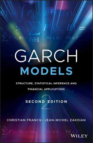
Let Ω* = {ω ∣ X 2t = 1, X 2t + 1 = 0, ∀ t}. If (X t ) is ergodic and stationary, the empirical means
 and
and  both converge to the same limit
P[X
t
= 1] with probability 1, by the ergodic theorem. For all
ω ∈ Ω*
these means are, respectively, equal to 1 and 0. Thus
P(Ω*) = 0. The probability of such a trajectory is thus equal to zero for any ergodic and stationary process.
both converge to the same limit
P[X
t
= 1] with probability 1, by the ergodic theorem. For all
ω ∈ Ω*
these means are, respectively, equal to 1 and 0. Thus
P(Ω*) = 0. The probability of such a trajectory is thus equal to zero for any ergodic and stationary process. - 1.5 We have
Eε
t
= 0, Var ε
t
= 1, and Cov(ε
t
, ε
t − h
) = 0 when
h ≠ 0, thus (ε
t
) is a weak white noise. We also have
 , thus ε
t
and ε
t − 1
are not independent, which shows that (ε
t
) is not a strong white noise.
, thus ε
t
and ε
t − 1
are not independent, which shows that (ε
t
) is not a strong white noise.
- 1.6 Assume
h > 0. Define the random variable
 where
where  . It is easy to see that
  has the same asymptotic variance (and also the same asymptotic distribution) as
  . Using
  , stationarity, and Lebesgue's theorem, this asymptotic variance is equal to
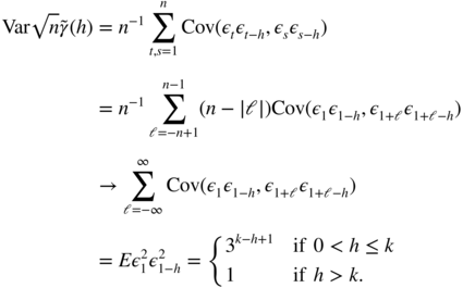
This value can be arbitrarily larger than 1, which is the value of the asymptotic variance of the empirical autocorrelations of a strong white noise.
- 1.7 It is clear that
 is a second‐order stationary process. By construction, ε
t
and ε
t − h
are independent when
h > k
, thus
is a second‐order stationary process. By construction, ε
t
and ε
t − h
are independent when
h > k
, thus  for all
h > k
. Moreover,
for all
h > k
. Moreover,  , for
h = 0, …, k
. In view of Theorem 1.2,
, for
h = 0, …, k
. In view of Theorem 1.2,  thus follows an MA(k) process. In the case
k = 1, we have
thus follows an MA(k) process. In the case
k = 1, we have
where ∣b∣ < 1 and (u t ) is a white noise of variance σ 2 . The coefficients b and σ 2 are determined by

which gives
 and
σ
2 = 2/b
.
and
σ
2 = 2/b
. - 1.8 Reasoning as in Exercise 1.6, the asymptotic variance is equal to

Since
 , for
k ≠ h
the asymptotic variance can be arbitrarily smaller than 1, which corresponds to the asymptotic variance of the empirical autocorrelations of a strong white noise.
, for
k ≠ h
the asymptotic variance can be arbitrarily smaller than 1, which corresponds to the asymptotic variance of the empirical autocorrelations of a strong white noise. - 1.9
- We havewhen n > m and m → ∞. The sequence {u t (n)} n defined by

 is a Cauchy sequence in
L
2
, and thus converges in quadratic mean. A priori,
is a Cauchy sequence in
L
2
, and thus converges in quadratic mean. A priori,
exists in ℝ ∪ + {∞}. Using Beppo Levi's theorem,

which shows that the limit
 is finite almost surely. Thus, as
n → ∞,
u
t
(n) converges, both almost surely and in quadratic mean, to
is finite almost surely. Thus, as
n → ∞,
u
t
(n) converges, both almost surely and in quadratic mean, to  . Since
we obtain, taking the limit as n → ∞ of both sides of the equality, u t = au t − 1 + η t . This shows that (X t ) = (u t ) is a stationary solution of the AR(1) equation.
Finally, assume the existence of two stationary solutions to the equation X t = aX t − 1 + η t and u t = au t − 1 + η t . If
 , then
which entails

This is in contradiction to the assumption that the two sequences are stationary, which shows the uniqueness of the stationary solution.
- We have
X
t
= η
t
+ aη
t − 1 + ⋯ + a
k
η
t − k
+ a
k + 1
X
t − k − 1
. Since ∣a ∣ = 1,

as k → ∞. If (X t ) were stationary,

and we would have

This is impossible, because by the Cauchy–Schwarz inequality,

- The argument used in Part 1 shows thatalmost surely and in quadratic mean. Since
 for all n , (
 ) is a stationary solution (which is called anticipative, because it is a function of the future values of the noise) of the AR(1) equation. The uniqueness of the stationary solution is shown as in Part 1.
 - The autocovariance function of the stationary solution is

We thus have Eε t = 0 and, for all h > 0,

which confirms that ε t is a white noise.
- We have
- 1.10 In Figure 1.6a, we note that several empirical autocorrelations are outside the 95% significance band, which leads us to think that the series may not be the realisation of a strong white noise. Inspection of Figure 1.6b confirms that the observed series ε1, …, ε
n
cannot be generated by a strong white noise; otherwise, the series
 would also be uncorrelated. Clearly, this is not the case, because several empirical autocorrelations go far beyond the significance band. By contrast, it is plausible that the series is a weak noise. We know that Bartlett's formula giving the limits
  is not valid for a weak noise (see Exercises 1.6 and 1.8). On the other hand, we know that the square of a weak noise can be correlated (see Exercise 1.7).
- 1.11 Using the relation
 , formula (B.18) can be written as
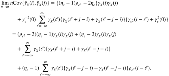
With the change of index h = i − ℓ, we obtain

which gives (B.14), using the parity of the autocovariance functions.
- 1.12 We can assume
i ≥ 0 and
j ≥ 0. Since
γ
X
(ℓ) = γ
ε(ℓ) = 0 for all ℓ ≠ 0, formula (B.18) yields

for (i, j) ≠ (0, 0) and

Thus

In formula (B.15), we have
 ij
= 0 when
i ≠ j
and
ij
= 0 when
i ≠ j
and  ii
= 1. We also have
ii
= 1. We also have  when
i ≠ j
and
when
i ≠ j
and  for all
i ≠ 0. Since
for all
i ≠ 0. Since  , we obtain
For significance intervals C h of asymptotic level 1 − α , such that
 , we have
By definition of C h ,

Moreover,

We have used the convergence in law of
 to a vector of independent variables. When the observed process is not a noise, this asymptotic independence does not hold in general.
 - 1.13 The probability that all the empirical autocorrelations stay within the asymptotic significance intervals (with the notation of the solution to Exercise 1.12) is, by the asymptotic independence,

For m = 20 and α = 5%, this limit is equal to 0.36. The probability of not rejecting the right model is thus low.
- 1.14 In view of (B.7), we have
r
X
(1) = ρ
X
(1). Using step (B.8) with
k = 2 and
a
1, 1 = ρ
X
(1), we obtain

Then, step (B.9) yields

Finally, step (B.8) yields

- 1.15 The historical data from 3 January 1950 to 24 July 2009 can be downloaded via the URL: http://fr.finance.yahoo.com/q/hp?s = %5EGSPC. We obtain Figure E.1 with the following R code:
> # reading the SP500 data set> sp500data <- read.table("sp500.csv",header=TRUE,sep=",")> sp500<-rev(sp500data$Close) # closing price> n<-length(sp500)> rend<-log(sp500[2:n]/sp500[1:(n-1)]); rend2<-rend∧2> op <- par(mfrow = c(2, 2)) # 2 × 2 figures per page> plot(ts(sp500),main="SP 500 from 1/3/50 to 7/24/09",+ ylab="SP500 Prices",xlab="")> plot(ts(rend),main="SP500 Returns",ylab="SP500 Returns",+ xlab="")> acf(rend, main="Autocorrelations of the returns",xlab="",+ ylim=c(-0.05,0.2))> acf(rend2, main="ACF of the squared returns",xlab="",+ ylim=c(-0.05,0.2))> par(op)
Figure E.1 Closing prices and returns of the S&P 500 index from 3 January 1950 to 24 July 2009.
Chapter 2
- 2.1 This covariance is meaningful only if
 and
Ef 2(ε
t − h
) < ∞. Under these assumptions, the equality is true and follows from
E(ε
t
∣ ε
u
, u < t) = 0.
and
Ef 2(ε
t − h
) < ∞. Under these assumptions, the equality is true and follows from
E(ε
t
∣ ε
u
, u < t) = 0.
- 2.2 In case (i) the strict stationarity condition becomes
α + β < 1. In case (ii) elementary integral computations show that the condition is

- 2.3 Let
λ
1, …, λ
m
be the eigenvalues of
A
. If
A
is diagonalisable, there exists an invertible matrix
P
and a diagonal matrix
D
such that
A = P
−1
DP
. It follows that, taking a multiplicative norm,
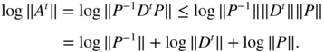
For the multiplicative norm ‖A‖ = ∑ ∣ a ij ∣, we have
 The result follows immediately.
When A is any square matrix, the Jordan representation can be used. Let n i be the multiplicity of the eigenvalue λ i . We have the Jordan canonical form A = P −1 JP , where P is invertible, and J is the block‐diagonal matrix with a diagonal of m matrices J i (λ i ), of size n i × n i , with λ i on the diagonal, 1 on the superdiagonal, and 0 elsewhere. It follows that A t = P −1 J t P , where J t is the block‐diagonal matrix whose blocks are the matrices
 . We have
  , where
N
i
is such that
, where
N
i
is such that  . It can be assumed that ∣λ
1 ∣ > ∣ λ
2 ∣ > ⋯ > ∣ λ
m
∣ . It follows that
. It can be assumed that ∣λ
1 ∣ > ∣ λ
2 ∣ > ⋯ > ∣ λ
m
∣ . It follows that
as t → ∞, and the proof easily follows.
- 2.4 We use the multiplicative norm ‖A‖ = ∑ ∣ a
ij
∣. Thus log‖Az
t
‖ ≤ log ‖A‖ + log ‖z
t
‖; therefore, log+‖Az
t
‖ ≤ log+ ‖A‖ + log+ ∣ z
t
∣, which admits a finite expectation by assumption. It follows that
γ
exists. We have

and thus

Using Eq. (2.21) and the ergodic theorem, we obtain

Consequently, γ < 0 if and only if ρ(A) < exp(−E log ∣ z t ∣).
- 2.5 To show 1, first note that, by stationarity, we have
 . The replacement can thus be done in (2.22). To show that it can also be done in (2.23), let us apply Theorem 2.3 to the sequence
  defined by
  . Noting that
  , we have
which completes the proof of 1.
We have shown that, for any
 , the stationary sequences
  and
and  have the same top Lyapunov exponent, i.e.
The convergence follows by showing that
 .
. - 2.5 For the Euclidean norm, multiplicativity follows from the Cauchy–Schwarz inequality. Since
 , we have
To show that the norm N 1 is not multiplicative, consider the matrix A whose elements are all equal to 1: we then have N 1(A) = 1 but N 1(A 2) > 1.
- 2.6 We have

and

- 2.7 We have
 , therefore, under the condition
α
1 + α
2 < 1, the moment of order 2 is given by
, therefore, under the condition
α
1 + α
2 < 1, the moment of order 2 is given by
(see Theorem 2.5 and Remark 2.6(1)). The strictly stationary solution satisfies

in ℝ ∪ {+∞}. Moreover,

which gives

Using this relation in the previous expression for
 , we obtain
If
 , then the term in brackets on the left‐hand side of the equality must be strictly positive, which gives the condition for the existence of the fourth‐order moment. Note that the condition is not symmetric in
α
1
and
α
2
. In Figure E.2, the points (α
1, α
2) under the curve correspond to ARCH(2) models with a fourth‐order moment. For these models,
, then the term in brackets on the left‐hand side of the equality must be strictly positive, which gives the condition for the existence of the fourth‐order moment. Note that the condition is not symmetric in
α
1
and
α
2
. In Figure E.2, the points (α
1, α
2) under the curve correspond to ARCH(2) models with a fourth‐order moment. For these models,

Figure E.2 Region of existence of the fourth‐order moment for an ARCH(2) model (when μ 4 = 3).
- 2.8 We have seen that
 admits the ARMA(1, 1) representation
where
 is a (weak) white noise. The author correlation of
  thus satisfiesE.1
Using the MA(∞) representation

we obtain

and

It follows that the lag 1 autocorrelation is
The other autocorrelations are obtained from (E.1) and
 . To determine the autocovariances, all that remains is to compute
which is given by

- 2.9 The vectorial representation
 is
is
We have

The eigenvalues of A (2) are 0, 0, 0 and 3α 2 + 2αβ + β 2 , thus I 4 − A (2) is invertible (0 is an eigenvalue of I 4 − A (2) if and only if 1 is an eigenvalue of A (2) ), and the system (2.63) admits a unique solution. We have
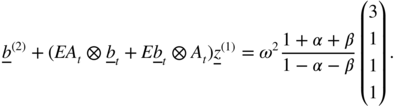
The solution to Eq. (2.63) is
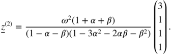
As first component of this vector, we recognise
 , and the other three components are equal to
  . Equation (2.64) yields
which gives
 , but with tedious computations, compared to the direct method utilised in Exercise 2.8.
 - 2.10 It suffices to show that
 for all fixed
  . Let
. Let  and
and  for
for  . For all
  , write
  with
with  . We have
and the result follows.
- 2.10
- Subtracting the (
q + 1)th line of (λI
p + q
− A) from the first, then expanding the determinant along the first row, and using Eq. (2.32), we obtainand the result follows.

- When
 the previous determinant is equal to zero at
λ = 1. Thus
ρ(A) ≥ 1. Now, let
λ
be a complex number of modulus strictly greater than 1. Using the inequality ∣a − b ∣ ≥ ∣ a ∣ − ∣ b∣, we then obtainIt follows that ρ(A) ≤ 1 and thus ρ(A) = 1.
the previous determinant is equal to zero at
λ = 1. Thus
ρ(A) ≥ 1. Now, let
λ
be a complex number of modulus strictly greater than 1. Using the inequality ∣a − b ∣ ≥ ∣ a ∣ − ∣ b∣, we then obtainIt follows that ρ(A) ≤ 1 and thus ρ(A) = 1.
- Subtracting the (
q + 1)th line of (λI
p + q
− A) from the first, then expanding the determinant along the first row, and using Eq. (2.32), we obtain
- 2.11 For all ε > 0, noting that the function
f(t) = P(t
−1 ∣ X
1 ∣ > ε) is decreasing, we have

The convergence follows from the Borel–Cantelli lemma.
Now, let (X n ) be an iid sequence of random variables with density f(x) = x −2
 x ≥ 1
. For all
K > 0, we have
x ≥ 1
. For all
K > 0, we have
The events {n −1 X n > K} being independent, we can use the counterpart of the Borel–Cantelli lemma: the event {n −1 X n > K for an infinite number of n} has probability 1. Thus, with probability 1, the sequence (n −1 X n ) does not tend to 0.
- 2.12 First note that the last
r − 1 lines of
B
t
A
are the first
r − 1 lines of
A
, for any matrix
A
of appropriate size. The same property holds true when
B
t
is replaced by
E(B
t
). It follows that the last
r − 1 lines of
E(B
t
A) are the last
r − 1 lines of
E(B
t
)E(A). Moreover, it can be shown, by induction on
t
, that the
i
th line ℓ
i, t − i
of
B
t
…B
1
is a measurable function of the
η
t − j
, for
j ≥ i
. The first line of
B
t + 1
B
t
…B
1
is thus of the form
a
1(η
t
)ℓ1, t − 1 + ⋯ + a
r
(η
t − r
)ℓ
r, t − r
. Since

the first line of EB t + 1 B t …B 1 is thus the product of the first line of EB t + 1 and of EB t …B 1 . The conclusion follows.
- 2.13
- For any fixed
t
, the sequence
 converges almost surely (to
  ) as
K → ∞. Thusand the first convergence follows. Now note that we have
) as
K → ∞. Thusand the first convergence follows. Now note that we have

The first inequality uses (a + b) s ≤ a s + b s for a, b ≥ 0 and s ∈ (0, 1]. The second inequality is a consequence of
 . The second convergence then follows from the dominated convergence theorem.
 - We have
 . The convergence follows from the previous question, and from the strict stationarity, for any fixed integer
K
, of the sequence
. The convergence follows from the previous question, and from the strict stationarity, for any fixed integer
K
, of the sequence  .
. - We have

for any i ′ = 1, …, ℓ, j ′ = 1, …, m . In view of the independence between X n and Y , it follows that
 almost surely as
n → ∞. Since
almost surely as
n → ∞. Since  is a strictly positive number, we obtain
  almost surely, for all
i
′, j
′
. Using (a + b)
s
≤ a
s
+ b
s
once again, it follows that
almost surely, for all
i
′, j
′
. Using (a + b)
s
≤ a
s
+ b
s
once again, it follows that
- Note that the previous question does not allow us to affirm that the convergence to 0 of
 entails that of
E(‖A
k
A
k − 1…A
1‖
s
), because
entails that of
E(‖A
k
A
k − 1…A
1‖
s
), because  has zero components. For
k
large enough, however, we have
has zero components. For
k
large enough, however, we have
where
 is independent of
A
k
A
k − 1…A
N + 1. The general term
a
i, j
of
A
N
…A
1
is the (i, j)th term of the matrix
A
N
multiplied by a product of
is independent of
A
k
A
k − 1…A
N + 1. The general term
a
i, j
of
A
N
…A
1
is the (i, j)th term of the matrix
A
N
multiplied by a product of  variables. The assumption
A
N
> 0 entails
a
i, j
> 0 almost surely for all
i
and
j
. It follows that the
i
th component of
Y
satisfies
Y
i
> 0 almost surely for all
i
. Thus
variables. The assumption
A
N
> 0 entails
a
i, j
> 0 almost surely for all
i
and
j
. It follows that the
i
th component of
Y
satisfies
Y
i
> 0 almost surely for all
i
. Thus  . Now the previous question allows to affirm that
E(‖A
k
A
k − 1…A
N + 1‖
s
) → 0 and, by strict stationarity, that
E(‖A
k − N
A
k − N − 1…A
1‖
s
) → 0 as
k → ∞. It follows that there exists
k
0
such that
. Now the previous question allows to affirm that
E(‖A
k
A
k − 1…A
N + 1‖
s
) → 0 and, by strict stationarity, that
E(‖A
k − N
A
k − N − 1…A
1‖
s
) → 0 as
k → ∞. It follows that there exists
k
0
such that 
- If
α
1
or
β
1
is strictly positive, the elements of the first two lines of the vector
 are also strictly positive, together with those of the (
q + 1)th and (
q + 2)th lines. By induction, it can be shown that
are also strictly positive, together with those of the (
q + 1)th and (
q + 2)th lines. By induction, it can be shown that  under this assumption.
 - The condition
 can be satisfied when
α
1 = β
1 = 0. It suffices to consider an ARCH(3) process with
α
1 = 0, α
2 > 0, α
3 > 0, and to check that
can be satisfied when
α
1 = β
1 = 0. It suffices to consider an ARCH(3) process with
α
1 = 0, α
2 > 0, α
3 > 0, and to check that  .
.
- For any fixed
t
, the sequence
- 2.14 In the case
p = 1, the condition on the roots of 1 − β
1
z
implies ∣β ∣ < 1. The positivity conditions on the
φ
i
yield
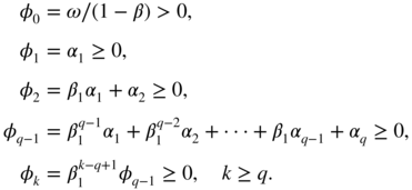
The last inequalities imply β 1 ≥ 0. Finally, the positivity constraints are

If q = 2, these constraints reduce to

Thus, we can have α 2 < 0.
- 2.15 Using the ARCH(
q
) representation of the process (
 ), together with Proposition 2.2, we obtain
- 2.16 Since
 ,
h > 0, we have
,
h > 0, we have  where
λ, μ
are constants and
r
1, r
2
satisfy
r
1 + r
2 = α
1
,
r
1
r
2 = − α
2
. It can be assumed that
r
2 < 0 and
r
1 > 0, for instance. A simple computation shows that, for all
h ≥ 0,
where
λ, μ
are constants and
r
1, r
2
satisfy
r
1 + r
2 = α
1
,
r
1
r
2 = − α
2
. It can be assumed that
r
2 < 0 and
r
1 > 0, for instance. A simple computation shows that, for all
h ≥ 0,
If the last equality is true, it remains true when h is replaced by h + 1 because
 . Since
  , it follows that
  for all
h ≥ 0. Moreover,
for all
h ≥ 0. Moreover,
Since
 , if
, if  then we have, for all
h ≥ 1,
then we have, for all
h ≥ 1,  We have thus shown that the sequence
  is decreasing when
  . If
. If  , it can be seen that for
h
large enough, say
h ≥ h
0
, we have
, it can be seen that for
h
large enough, say
h ≥ h
0
, we have  , again because of
  . Thus, the sequence
  is decreasing.
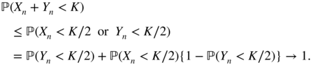
 - 2.17 Since
X
n
+ Y
n
→ − ∞ in probability, for all
K
we have
Since
 in probability, there exist
K
0 ∈ ℝ and
n
0 ∈ ℕ such that
P(X
n
< K
0/2) ≤ ς < 1 for all
n ≥ n
0
. Consequently,
in probability, there exist
K
0 ∈ ℝ and
n
0 ∈ ℕ such that
P(X
n
< K
0/2) ≤ ς < 1 for all
n ≥ n
0
. Consequently,
as n → ∞, for all K ≤ K 0 , which entails the result.
- 2.18 We have

as n → ∞. If γ < 0, the Cauchy rule entails that

converges almost surely, and the process (ε t ), defined by
 , is a strictly stationary solution of model (2.7). As in the proof of Theorem 2.1, it can be shown that this solution is unique, non‐anticipative and ergodic. The converse is proved by contradiction, assuming that there exists a strictly stationary solution
  . For all
n > 0, we have
. For all
n > 0, we have
It follows that a(η −1)…a(η −n )ω(η −n − 1) converges to zero, almost surely, as n → ∞ , or, equivalently, that
E.2
We first assume that E log {a(η t )} > 0. Then the strong law of large numbers entails
 almost surely. For (E.2) to hold true, it is then necessary that log ω(η
−n − 1) → − ∞ almost surely, which is precluded since (η
t
) is iid and
ω(η
0) > 0 almost surely. Assume now that
E log {a(η
t
)} = 0. By the Chung–Fuchs theorem, we have
almost surely. For (E.2) to hold true, it is then necessary that log ω(η
−n − 1) → − ∞ almost surely, which is precluded since (η
t
) is iid and
ω(η
0) > 0 almost surely. Assume now that
E log {a(η
t
)} = 0. By the Chung–Fuchs theorem, we have  with probability 1 and, using Exercise 2.17, the convergence (E.2) entails log ω(η
−n − 1) → − ∞ in probability, which, as in the previous case, entails a contradiction.
with probability 1 and, using Exercise 2.17, the convergence (E.2) entails log ω(η
−n − 1) → − ∞ in probability, which, as in the previous case, entails a contradiction. - 2.19 Letting
a(z) = λ + (1 − λ)z
2
, we have

Regardless of the value of
 , fixed or even random, we have almost surely
using the law of large numbers and Jensen's inequality. It follows that
 almost surely as
t → ∞.
almost surely as
t → ∞. - 2.20
- Since the φ i are positive and A 1 = 1, we have φ i ≤ 1, which shows the first inequality. The second inequality follows by convexity of x ↦ x log x for x > 0.
- Since
A
1 = 1 and
A
p
< ∞, the function
f
is well defined for
q ∈ [p, 1]. We haveThe function q ↦ log E|η 0|2q is convex on [p,1] if, for all λ ∈ [0, 1] and all q, q * ∈ [p, 1],


which is equivalent to showing that

with X = |η 0|2q ,
 . This inequality holds true by Hölder's inequality. The same argument is used to show the convexity of
  . It follows that
f
is convex, as a sum of convex functions. We have
f(1) = 0 and
f(p) < 0, thus the left derivative of
f
at 1 is negative, which gives the result.
. It follows that
f
is convex, as a sum of convex functions. We have
f(1) = 0 and
f(p) < 0, thus the left derivative of
f
at 1 is negative, which gives the result. - Conversely, we assume that there exists
p
* ∈ (0, 1] such that
 and that condition (2.52) is satisfied. The convexity of
f
on [p
*, 1] and (2.52) implies that
f(q) < 0 for
q
sufficiently close to 1. Thus condition (2.41) is satisfied. By convexity of
f
and since
f(1) = 0, we have
f(q) < 0 for all
q ∈ [p, 1]. It follows that, by Theorem 2.6,
E|ε
t
|
q
< ∞ for all
q ∈ [0, 2].
and that condition (2.52) is satisfied. The convexity of
f
on [p
*, 1] and (2.52) implies that
f(q) < 0 for
q
sufficiently close to 1. Thus condition (2.41) is satisfied. By convexity of
f
and since
f(1) = 0, we have
f(q) < 0 for all
q ∈ [p, 1]. It follows that, by Theorem 2.6,
E|ε
t
|
q
< ∞ for all
q ∈ [0, 2].
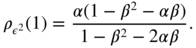
- 2.21 Since
 , we have
a = 0 and
b = 1. Using condition (2.60), we can easily see that
, we have
a = 0 and
b = 1. Using condition (2.60), we can easily see that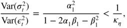
since the condition for the existence of
 is
is  . Note that when the GARCH effect is weak (that is,
α
1
is small), the part of the variance that is explained by this regression is small, which is not surprising. In all cases, the ratio of the variances is bounded by 1/κ
η
, which is largely less than 1 for most distributions (1/3 for the Gaussian distribution). Thus, it is not surprising to observe disappointing
R
2
values when estimating such a regression on real series.
. Note that when the GARCH effect is weak (that is,
α
1
is small), the part of the variance that is explained by this regression is small, which is not surprising. In all cases, the ratio of the variances is bounded by 1/κ
η
, which is largely less than 1 for most distributions (1/3 for the Gaussian distribution). Thus, it is not surprising to observe disappointing
R
2
values when estimating such a regression on real series.
Chapter 3
- 3.1
Given any initial measure, the sequence (X
t
)
t ∈ ℕ
clearly constitutes a Markov chain on (ℝ, ℬ(ℝ)), with transition probabilities defined by
P(x, B) = ℙ(X
1 ∈ B ∣ X
0 = x) = P
ε
(B − θx).
- (a) Since
P
ε
admits a positive density on ℝ, the probability measure
P(x, .) is, for all
x ∈ E
, absolutely continuous with respect to
λ
and its density is positive on ℝ. Thus any measure
ϕ
which is absolutely continuous with respect to
λ
is a measure of irreducibility: ∀x ∈ E
,

Moreover, λ is a maximal measure of irreducibility.
- (b) Assume, for example, that ε t is uniformly distributed on [−1, 1]. If θ > 1 and X 0 = x 0 > 1/(θ − 1), we have x 0 < X 1 < X 2 < …, regardless of the ε t . Thus there exists no irreducibility measure: such a measure should satisfy ϕ([ − ∞ , x]) = 0, for all x ∈ ℝ, which would imply ϕ = 0.
- (a) Since
P
ε
admits a positive density on ℝ, the probability measure
P(x, .) is, for all
x ∈ E
, absolutely continuous with respect to
λ
and its density is positive on ℝ. Thus any measure
ϕ
which is absolutely continuous with respect to
λ
is a measure of irreducibility: ∀x ∈ E
,
- 3.2 If (X
n
) is strictly stationary,
X
1
and
X
0
have the same distribution,
μ
, satisfying

Thus μ is an invariant probability measure.
Conversely, suppose that μ is invariant. Using the Chapman–Kolmogorov relation, by which ∀t ∈ ℕ, ∀ s, 0 ≤ s ≤ t, ∀ x ∈ E, ∀ B ∈ ℰ,

we obtain

Thus, by induction, for all t , ℙ[X t ∈ B] = μ(B) (∀B ∈ ℬ ). Using the Markov property, this is equivalent to the strict stationarity of the chain: the distribution of the process (X t , X t + 1, …, X t + k ) is independent of t , for any integer k .
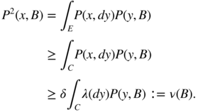
- 3.3 We have

Thus π is invariant. The third equality is an immediate consequence of the Fubini and Lebesgue theorems.
- 3.4 Assume, for instance,
θ > 0. Let
C = [−c, c],
c > 0, and let
δ = inf {f(x); x ∈ [−(1 + θ)c, (1 + θ)c]} We have, for all
A ⊂ C
and all
x ∈ C
,

Now let B ∈ ℰ . Then for all x ∈ C ,
The measure ν is non‐trivial since ν(E) = δλ(C) = 2δc > 0.
- 3.5 It is clear that (X
t
) constitutes a Feller chain on ℝ. The
λ
‐irreducibility follows from the assumption that the noise has a density which is everywhere positive, as in Exercise 3.1. In order to apply Theorem 3.1, a natural choice of the test function is
V(x) = 1 + ∣ x∣. We have

Thus if K 1 < 1, we have, for K 1 < K < 1 and for g(x) > (K 2 + 1 − K 1)/(K − K 1),

If we put A = {x; g(x) = 1 + ∣ x ∣ ≤ (K 2 + 1 − K 1)/(K − K 1)}, the set A is compact and the conditions of Theorem 3.1 are satisfied, with 1 − δ = K .
- 3.6 By summing the first
n
inequalities of (3.11) we obtain

It follows that

because V ≥ 1. Thus, there exists κ > 0 such that

Note that the positivity of δ is crucial for the conclusion.
- 3.7 We have, for any positive continuous function
f
with compact support,

The inequality is justified by (i) and the fact that P f is a continuous positive function. It follows that for f =
 C
, where
C
is a compact set, we obtain
C
, where
C
is a compact set, we obtain
which shows that,

(that is, π is subvarient) using (ii). If there existed B such that the previous inequality were strict, we should have

and since π(E) < ∞ we arrive at a contradiction. Thus

which signifies that π is invariant.
- 3.8 See Francq and Zakoïan (2006b).
- 3.9 If
 were infinite then, for any
K > 0, there would exist a subscript
n
0
such that
were infinite then, for any
K > 0, there would exist a subscript
n
0
such that  . Then, using the decrease in the sequence, one would have
  . Since this should be true for all
K > 0, the sequence would not converge. This applies directly to the proof of Corollary A.3 with
u
n
= {α
X
(n)}
ν/(2 + ν)
, which is indeed a decreasing sequence in view of point (v) on Section A.3.1.
. Since this should be true for all
K > 0, the sequence would not converge. This applies directly to the proof of Corollary A.3 with
u
n
= {α
X
(n)}
ν/(2 + ν)
, which is indeed a decreasing sequence in view of point (v) on Section A.3.1.
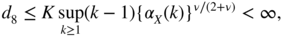
- 3.10 We have

where

Inequality (A.8) shows that d 7 is bounded by

By an argument used to deal with d 6 , we obtain
and the conclusion follows.
- 3.11 The chain satisfies the Feller condition (i) because
is continuous at x when g is continuous.
To show that the irreducibility condition (ii) is not satisfied, consider the set of numbers in [0,1] such that the sequence of decimals is periodic after a certain lag:

For all h ≥ 0,
 if and only if
  . We thus have,
and,

This shows that there is no non‐trivial irreducibility measure.
The drift condition (iii) is satisfied with, for instance, a measure φ such that φ([−1, 1]) > 0, the energy V(x) = 1 + ∣ x∣ and the compact set A = [−1, 1]. Indeed,

provided

Chapter 4
- 4.1
Note that
 is a measurable function of
  and of
  , that will be denoted by
Using the independence between
 and the other variables of
  , we have, for all
  ,
,
when the distribution
 is symmetric.
 - 4.2 A sequence
 of independent real random variables such that
  with probability
  and
and  with probability
  is suitable, because
  ,
,  ,
,  and
and  . We have used
  for any decreasing sequence of events, in order to show that
- 4.3 By definition,
and, by continuity of the exponential,
is finite if and only if the series of general term
 converges. Using the inequalities
  , we obtain
Since the
 tend to 0 at an exponential rate and
  , the series of general term
  converges absolutely, and we finally obtain
which is finite under condition (4.12).
- 4.4 Note that (4.13) entails that

with probability 1. The integral of a positive measurable function being always defined in
 , using Beppo Levi's theorem and then the independence of the
  , we obtain
which is of course finite under condition (4.12). Applying the dominated convergence theorem, and bounding the variables
 by the integrable variable
  , we then obtain the desired expression for
  .
. - 4.5 Denoting by
 the density of
  ,
,
and
 . With the notation
  , it follows that
It then suffices to use the fact that
 is equivalent to
  , and that
  is thus equivalent to
  , in a neighborhood of 0.
 - 4.6 We can always assume
 . In view of the discussion on pages 79–80, the process
  satisfies an ARMA
 representation of the form
where
 is a white noise with variance
  . Using
  and
and
the coefficients
 and
and  are such that
and

When, for instance,
 ,
,  ,
,  and
and  , we obtain
- 4.7 In view of Exercise 3.5, an AR
 process
  ,
,  , in which the noise
  has a strictly positive density over
  , is geometrically
  ‐mixing. Under the stationarity conditions given in Theorem 4.1, if
  has a density
  and if
  (defined in (4.10)) is a continuously differentiable bijection (that is, if
  ) then
  is a geometrically
  ‐mixing stationary process. Reasoning as in step (iv) of the proof of Theorem 3.4, it is shown that
  , and then
  , are also geometrically
  ‐mixing stationary processes.
- 4.8 Since
 and
and  , we have
If the volatility
 is a positive function of
  that possesses a moment of order 2, then
under conditions (4.34). Thus, condition (4.38) is necessarily satisfied. Conversely, under (4.38) the strict stationarity condition is satisfied because

and, as in the proof of Theorem 2.2, it is shown that the strictly stationary solution possesses a moment of order 2.
- 4.9 Assume the second‐order stationarity condition (4.39). Let
and

Using
 , we obtain
We then obtain the autocovariances

and the autocorrelations
 . Note that
  for all
  , which shows that
  is a weak ARMA
 process. In the standard GARCH case, the calculation of these autocorrelations would be much more complicated because
  is not a linear function of
  .
. - 4.10 This is obvious because an APARCH
 with
with  ,
,  and
and  corresponds to a TGARCH
 .
.
- 4.11 This is an EGARCH
 with
with  ,
,  ,
,  and
and  . It is natural to impose
  and
and  , so that the volatility increases with
  . It is also natural to impose
  so that the effect of a negative shock is more important than the effect of a positive shock of the same magnitude. There always exists a strictly stationary solution
and this solution possesses a moment of order 2 when

which is the case, in particular, for
 . In the Gaussian case, we have
and

using the calculations of Exercise 4.5 and

Since
 is an increasing function, provided
  , we observe the leverage effect
  .
. - 4.12 For all
ε > 0, we have

and the conclusion follows from the Borel–Cantelli lemma.
- 4.13 Because the increments of the Brownian motion are independent and Gaussian, we have
and

as h → 0. The conclusion follows.
- 4.14 We have

Using the indication, one can check that
 and
and
We thus conclude by noting that

Chapter 5
- Let (ℱ
t
) be an increasing sequence of
σ
‐fields such that ε
t
∈ ℱ
t
and
E(ε
t
∣ ℱ
t − 1) = 0. For
h > 0, we have ε
t
ε
t + h
∈ ℱ
t + h
and

The sequence (ε t ε t + h , ℱ t + h ) t is thus a stationary sequence of square integrable martingale increments. We thus have

where
 . To conclude,
1
it suffices to note that
. To conclude,
1
it suffices to note that
in probability (and even in L 2 ).
- 5.2 This process is a stationary martingale difference, whose variance is

Its fourth‐order moment is

Thus,

Moreover,

Using Exercise 5.1, we thus obtain

- 5.3 We have

By the ergodic theorem, the denominator converges in probability (and even a.s.) to γ ε(0) = ω/(1 − α) ≠ 0. In view of Exercise 5.2, the numerator converges in law to
 . Cramér's theorem
2
then entails
. Cramér's theorem
2
then entails
The asymptotic variance is equal to 1 when α = 0 (that is, when ε t is a strong white noise). Figure E.3 shows that the asymptotic distribution of the empirical autocorrelations of a GARCH can be very different from those of a strong white noise.

Figure E.3 Comparison between the asymptotic variance of
 for the ARCH(1) process (5.28) with (η
t
) Gaussian (solid line) and the asymptotic variance of
for the ARCH(1) process (5.28) with (η
t
) Gaussian (solid line) and the asymptotic variance of  when ε
t
is a strong white noise (dashed line).
when ε
t
is a strong white noise (dashed line). - 5.4 Using Exercise 2.8, we obtain

In view of Exercises 5.1 and 5.3,

for any h ≠ 0.
- 5.5 Let ℱ
t
be the
σ
‐field generated by {η
u
, u ≤ t}. If
s + 2 > t + 1, then

Similarly, Eε t ε t + 1ε s ε s + 2 = 0 when t + 1 > s + 2. When t + 1 = s + 2, we have

because ε t − 1 σ t ∈ ℱ t − 1 ,
 ,
E(η
t
∣ ℱ
t − 1) = Eη
t
= 0 and
,
E(η
t
∣ ℱ
t − 1) = Eη
t
= 0 and  . Using (7.24), the result can be extended to show that
Eε
t
ε
t + h
ε
s
ε
s + k
= 0 when
k ≠ h
and (ε
t
) follows a GARCH(p, q), with a symmetric distribution for
η
t
.
. Using (7.24), the result can be extended to show that
Eε
t
ε
t + h
ε
s
ε
s + k
= 0 when
k ≠ h
and (ε
t
) follows a GARCH(p, q), with a symmetric distribution for
η
t
. - 5.6 Since
Eε
t
ε
t + 1 = 0, we have Cov{ε
t
ε
t + 1, ε
s
ε
s + 2} = Eε
t
ε
t + 1ε
s
ε
s + 2 = 0 in view of Exercise 5.5. Thus

- 5.7 In view of Exercise 2.8, we have

with ω = 1, α = 0.3 and β = 0.55. Thus γ ε(0) = 6.667,
 ,
,  . Thus
for i = 1, …, 5. Finally, using Theorem 5.1,

- 5.8 Since
γ
X
(ℓ) = 0, for all ∣ℓ ∣ > q
, we clearly have

Since
 ,
γ
ε(0) = ω/(1 − α) and
,
γ
ε(0) = ω/(1 − α) and
(see, for instance, Exercise 2.8), we have

Note that
 as
i → ∞.
as
i → ∞. - 5.9 Conditionally on initial values, the score vector is given by

where ε t (θ) = Y t − F θ (W t ). We thus have

and, when σ 2 does not depend on θ ,

- 5.10 In the notation of Section 5.4.1 and denoting by
 the parameter of interest, the log‐likelihood is equal to
up to a constant. The constrained estimator is
 , with
  . The constrained score and the Lagrange multiplier are related by
On the other hand, the exact laws of the estimators under H 0 are given by

and

with

For the case
 , we can estimate
I
22
by
, we can estimate
I
22
by
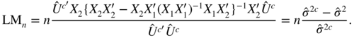
The test statistic is then equal to
E.3
with

and where R 2 is the coefficient of determination (centred if X 1 admits a constant column) in the regression of
 on the columns of
X
2
. For the first equality of (E.3), we use the fact that in a regression model of the form
Y = Xβ + U
, with obvious notation, Pythagoras's theorem yields
on the columns of
X
2
. For the first equality of (E.3), we use the fact that in a regression model of the form
Y = Xβ + U
, with obvious notation, Pythagoras's theorem yields
In the general case, we have
Since the residuals of the regression of Y on the columns of X 1 and X 2 are also the residuals of the regression of
 on the columns of
X
1
and
X
2
, we obtain LM
n
by:
on the columns of
X
1
and
X
2
, we obtain LM
n
by:- computing the residuals
 of the regression of
Y
on the columns of
X
1
;
of the regression of
Y
on the columns of
X
1
; - regressing
 on the columns of
X
2
and
X
1
, and setting LM
n
= nR
2
, where
R
2
is the coefficient of determination of this second regression.
on the columns of
X
2
and
X
1
, and setting LM
n
= nR
2
, where
R
2
is the coefficient of determination of this second regression.
- computing the residuals
- 5.11 Since
 , it is clear that
  , with
  and
R
2
defined in representations (5.29) and (5.30).
and
R
2
defined in representations (5.29) and (5.30).Since T is invertible, we have
 , where Col(Z) denotes the vectorial subspace generated by the columns of the matrix
Z
, and
, where Col(Z) denotes the vectorial subspace generated by the columns of the matrix
Z
, and
If e ∈ Col(X) then
 and
and
Noting that
 , we conclude that
Chapter 6
- From the observations ε1, …, ε
n
, we can compute
 and
and
for h = 0, …, q . We then put

and then, for k = 2, …, q (when q > 1),

With standard notation, the OLS estimators are then

- 6.2 The assumption that
X
has full column rank implies that
X
′
X
is invertible. Denoting by 〈⋅, ⋅〉 the scalar product associated with the Euclidean norm, we have

and

with equality if and only if
 , and we are done.
 - 6.3 We can take
n = 2,
q = 1, ε0 = 0, ε1 = 1, ε2 = 0. The calculation yields
 .
.
- 6.4 Case 3 is not possible, otherwise we would have

for all t , and consequently
 , which is not possible.
Using the data, we obtain
 , and thus
  . Therefore, the constrained estimate must coincide with one of the following three constrained estimates: that constrained by
α
2 = 0, that constrained by
α
1 = 0, or that constrained by
α
1 = α
2 = 0. The estimate constrained by
α
2 = 0 is
. Therefore, the constrained estimate must coincide with one of the following three constrained estimates: that constrained by
α
2 = 0, that constrained by
α
1 = 0, or that constrained by
α
1 = α
2 = 0. The estimate constrained by
α
2 = 0 is  , and thus does not suit. The estimate constrained by
α
1 = 0 yields the desired estimate
, and thus does not suit. The estimate constrained by
α
1 = 0 yields the desired estimate  .
. - 6.5 First note that
 . Thus
  if and only if
η
t
= 0. The nullity of the
i
th column of
X
, for
i > 1, implies that
η
n − i + 1 = ⋯ = η
2 = η
1 = 0. The probability of this event tends to 0 as
n → ∞ because, since
if and only if
η
t
= 0. The nullity of the
i
th column of
X
, for
i > 1, implies that
η
n − i + 1 = ⋯ = η
2 = η
1 = 0. The probability of this event tends to 0 as
n → ∞ because, since  , we have
P(η
t
= 0) < 1.
, we have
P(η
t
= 0) < 1.
- 6.6 Introducing an initial value
X
0
, the OLS estimator of
φ
0
is

and this estimator satisfies

Under the assumptions of the exercise, the ergodic theorem entails the almost sure convergence

and thus the almost sure convergence of
 to
φ
0
. For the consistency, the assumption
to
φ
0
. For the consistency, the assumption  suffices.
If
 , the sequence (ε
t
X
t − 1, ℱ
t
) is a stationary and ergodic square integrable martingale difference, with variance
, the sequence (ε
t
X
t − 1, ℱ
t
) is a stationary and ergodic square integrable martingale difference, with variance
We can see that this expectation exists by expanding the product

The CLT of Corollary A.1 then implies that

and thus

When
 , the condition
  suffices for asymptotic normality.
 - 6.7 By direct verification, A −1 A = I .
- 6.8
- Let
 Then
Then  solves the modelThe parameter ω 0 vanishing in this equation, the moments of
 do not depend on it. It follows that
- and 3. Write
 to indicate that a matrix
M
is proportional to
to indicate that a matrix
M
is proportional to  . Partition the vector
  into
Z
t − 1 = (1, W
t − 1)′
and, accordingly, the matrices
A
and
B
of Theorem 6.2. Using the previous question and the notation of Exercise 6.7, we obtain
into
Z
t − 1 = (1, W
t − 1)′
and, accordingly, the matrices
A
and
B
of Theorem 6.2. Using the previous question and the notation of Exercise 6.7, we obtain
We then have

Similarly,

It follows that C = A −1 BA −1 is of the form

- Let
- 6.9
- Let
 Let us show the existence of
x
*
. Let (x
n
) be a sequence of elements of
C
such that, for all
n > 0, ‖x − x
n
‖2 < α
2 + 1/n
. Using the parallelogram identity ‖a + b‖2 + ‖a − b‖2 = 2‖a‖2 + 2‖b‖2
, we havethe last inequality being justified by the fact that (x m + x n )/2 ∈ C , the convexity of C and the definition of α . It follows that (x n ) is a Cauchy sequence and, E being a Hilbert space and therefore a complete metric space, x n converges to some point x * . Since C is closed, x * ∈ C and ‖x − x *‖ ≥ α . We have also ‖x − x *‖ ≤ α , taking the limit on both sides of the inequality which defines the sequence (x n ). It follows that ‖x − x *‖ = α , which shows the existence.
Let us show the existence of
x
*
. Let (x
n
) be a sequence of elements of
C
such that, for all
n > 0, ‖x − x
n
‖2 < α
2 + 1/n
. Using the parallelogram identity ‖a + b‖2 + ‖a − b‖2 = 2‖a‖2 + 2‖b‖2
, we havethe last inequality being justified by the fact that (x m + x n )/2 ∈ C , the convexity of C and the definition of α . It follows that (x n ) is a Cauchy sequence and, E being a Hilbert space and therefore a complete metric space, x n converges to some point x * . Since C is closed, x * ∈ C and ‖x − x *‖ ≥ α . We have also ‖x − x *‖ ≤ α , taking the limit on both sides of the inequality which defines the sequence (x n ). It follows that ‖x − x *‖ = α , which shows the existence.
Assume that there exist two solutions of the minimisation problem in C ,
 and
and  . Using the convexity of
C
, it is then easy to see that
. Using the convexity of
C
, it is then easy to see that  satisfies
This is possible only if
 (once again using the parallelogram identity).
 - Let
λ ∈ (0, 1) and
y ∈ C
. Since
C
is convex, (1 − λ)x
* + λy ∈ C
. Thus

and, dividing by λ ,

Taking the limit as λ tends to 0, we obtain inequality (6.17).
Let z such that, for all y ∈ C , 〈z − x, z − y〉 ≤ 0. We have

the last inequality being simply the Cauchy–Schwarz inequality. It follows that ‖x − z‖ ≤ ‖x − y‖, ∀ y ∈ C . This property characterising x * in view of part 1, it follows that z = x * .
- Let
- 6.10
- It suffices to show that when C = K , (6.17) is equivalent to (6.18). Since 0 ∈ K , taking y = 0 in (6.17) we obtain 〈x − x *, x *〉 ≤ 0. Since x * ∈ K and K is a cone, 2x * ∈ K . For y = 2x * in (6.17) we obtain 〈x − x *, x *〉 ≥ 0, and it follows that 〈x − x *, x *〉 = 0. The second equation of (6.18) then follows directly from (6.17). The converse, (6.18) ⇒ (6.17), is trivial.
- Since
x
* ∈ K
, then
z = λx
* ∈ K
for
λ ≥ 0. By (6.18), we haveIt follows that (λx)* = z and (a) is shown. The properties (b) are obvious, expanding ‖x * + (x − x *)‖2 and using the first equation of (6.18).
- 6.11 The model is written as
Y = X
(1)
θ
(1) + X
(2)
θ
(2) + U. Thus, since
M
2
X
(2) = 0, we have
M
2
Y = M
2
X
(1)
θ
(1) + M
2
U. Note that this is a linear model, of parameter
θ
(1)
. Noting that
 , since
M
2
is an orthogonal projection matrix, the form of the estimator follows.
, since
M
2
is an orthogonal projection matrix, the form of the estimator follows.
- 6.12 Since
J
n
is symmetric, there exists a diagonal matrix
D
n
and an orthonormal matrix
P
n
such that
 . For
n
large enough, the eigenvalues of
J
n
are positive since
. For
n
large enough, the eigenvalues of
J
n
are positive since  is positive definite. Let
λ
n
be the smallest eigenvalue of
J
n
. Denoting by ‖ ⋅ ‖ the Euclidean norm, we have
is positive definite. Let
λ
n
be the smallest eigenvalue of
J
n
. Denoting by ‖ ⋅ ‖ the Euclidean norm, we have
Since
 and
and  , it follows that
  , and thus that
X
n
converges to the zero vector of ℝ
k
.
, and thus that
X
n
converges to the zero vector of ℝ
k
. - 6.13 Applying the method of Section 6.3.2, we obtain
X
(1) = (1, 1)′
and thus, by Theorem 6.8,

Chapter 7
-
- When j < 0, all the variables involved in the expectation, except ε t − j , belong to the σ ‐field generated by {ε t − j − 1, ε t − j − 2, …}. We conclude by taking the expectation conditionally on the previous σ ‐field and using the martingale increment property.
- For
j ≥ 0, we note that
 is a measurable function of
  and of
  Thus
Thus  is an even function of the conditioning variables, denoted by
  .
. - It follows that the expectation involved in the property can be written asThe latter equality follows from of the nullity of the integral, because the distribution of η t is symmetric.
- 7.2 By the Borel–Cantelli lemma, it suffices to show that for all real
δ > 0, the series of general terms
 converges. That is to say,
using Markov's inequality, strict stationarity and the existence of a moment of order s > 0 for
 .
. - 7.3 For all
κ > 0, the process
 is ergodic and admits an expectation. This expectation is finite since
  and
and  . We thus have, by the standard ergodic theorem,
When κ → ∞, the variable
 increases to
X
1
. Thus by Beppo Levi's theorem
increases to
X
1
. Thus by Beppo Levi's theorem  converges to
E(X
1) = + ∞. It follows that
converges to
E(X
1) = + ∞. It follows that  tends almost surely to infinity.
 - 7.4
- The assumptions made on
f
and Θ guarantee that
 is a measurable function of
η
t
, η
t − 1, …. By Theorem A.1, it follows that (Y
t
) is stationary and ergodic.
is a measurable function of
η
t
, η
t − 1, …. By Theorem A.1, it follows that (Y
t
) is stationary and ergodic. - If we remove condition (7.94), the property may not be satisfied. For example, let Θ = {θ
1, θ
2} and assume that the sequence (X
t
(θ
1), X
t
(θ
2)) is iid, with zero mean, each component being of variance 1 and the covariance between the two components being different when
t
is even and when
t
is odd. Each of the two processes (X
t
(θ
1)) and (X
t
(θ
2)) is stationary and ergodic (as iid processes). However,
 is not stationary in general because its distribution depends on the parity of
t
.
is not stationary in general because its distribution depends on the parity of
t
.
- The assumptions made on
f
and Θ guarantee that
- 7.5
- In view of (7.30) and of the second part of assumption A1, we haveE.7almost surely. Indeed, on a set of probability 1, we have for all ι > 0,
 E.8
E.8
Note that
 and (7.29) entail that
  . The limit superior (E.5) being less than any positive number, it is null.
 - Note that
 is the strong innovation of
  . We thus have orthogonality between
ν
t
and any integrable variable which is measurable with respect to the
σ
‐field generated by θ0
:with equality if and only if
. We thus have orthogonality between
ν
t
and any integrable variable which is measurable with respect to the
σ
‐field generated by θ0
:with equality if and only if

 ‐almost surely, that is,
θ = θ
0
(by assumptions A3 and A4; see the proof of Theorem 7.1).
‐almost surely, that is,
θ = θ
0
(by assumptions A3 and A4; see the proof of Theorem 7.1). - We conclude that
 is strongly consistent, as in (d) in the proof of Theorem 7.1, using a compactness argument and applying the ergodic theorem to show that, at any point
θ
1
, there exists a neighbourhood
V(θ
1) of
θ
1
such that
is strongly consistent, as in (d) in the proof of Theorem 7.1, using a compactness argument and applying the ergodic theorem to show that, at any point
θ
1
, there exists a neighbourhood
V(θ
1) of
θ
1
such that
- Since all we have done remains valid when Θ is replaced by any smaller compact set containing
θ
0
, for instance Θ
c
, the estimator
 is strongly consistent.
- In view of (7.30) and of the second part of assumption A1, we have
- 7.6 We know that
 minimises, over Θ,
For all c > 0, there exists
 such that
  for all
t ≥ 0. Note that
for all
t ≥ 0. Note that  if and only if
c ≠ 1. For instance, for a GARCH(1, 1) model, if
if and only if
c ≠ 1. For instance, for a GARCH(1, 1) model, if  we have
  . Let
. Let  The minimum of
f
is obtained at the unique point
The minimum of
f
is obtained at the unique point
If
 , we have
  . It follows that
c
0 = 1 with probability 1, which proves the result.
. It follows that
c
0 = 1 with probability 1, which proves the result. - 7.7 The expression for
I
1
is a trivial consequence of (7.74) and Cov
 . Similarly, the form of
I
2
directly follows from (7.38). Now consider the non‐diagonal blocks. Using (7.38) and (7.74), we obtain
. Similarly, the form of
I
2
directly follows from (7.38). Now consider the non‐diagonal blocks. Using (7.38) and (7.74), we obtain
In view of (7.41), (7.42), (7.79) and (7.24), we have

and

It follows that
E.6
and ℐ is block‐diagonal. It is easy to see that 풥 has the form given in the theorem. The expressions for J 1 and J 2 follow directly from (7.39) and (7.75). The block‐diagonal form follows from (7.76) and (E.6).
- 7.8
- We have
 The parameters to be estimated are
a
and
α
,
ω
being known. We haveIt follows that
The parameters to be estimated are
a
and
α
,
ω
being known. We haveIt follows that

Letting ℐ = (ℐ ij ),
 and
and  , we then obtain
- In the case where the distribution of
η
t
is symmetric we have
μ
3 = 0 and, using (7.24),
 . It follows that
The asymptotic variance of the ARCH parameter estimator is thus equal to
 : it does not depend on
a
0
and is the same as that of the QMLE of a pure ARCH(1) (using computations similar to those used to obtain (7.1.2)).
: it does not depend on
a
0
and is the same as that of the QMLE of a pure ARCH(1) (using computations similar to those used to obtain (7.1.2)). - When
α
0 = 0, we have
 , and thus
  . It follows that

We note that the estimation of too complicated a model (since the true process is AR(1) without ARCH effect) does not entail any asymptotic loss of accuracy for the estimation of the parameter a 0 : the asymptotic variance of the estimator is the same,
 , as if the AR(1) model were directly estimated. This calculation also allows us to verify the ‘
α
0 = 0’ column in Table 7.3: for the
, as if the AR(1) model were directly estimated. This calculation also allows us to verify the ‘
α
0 = 0’ column in Table 7.3: for the  law we have
μ
3 = 0 and
κ
η
= 3; for the normalized
χ
2(1) distribution we find
law we have
μ
3 = 0 and
κ
η
= 3; for the normalized
χ
2(1) distribution we find  and
κ
η
= 15.
and
κ
η
= 15.
- We have
- 7.9 Let
ε > 0 and
V(θ
0) be such that (7.95) is satisfied. Since
 almost surely, for
n
large enough
almost surely, for
n
large enough  almost surely. We thus have almost surely
It follows that

and, since ε can be chosen arbitrarily small, we have the desired result.
In order to give an example where (7.95) is not satisfied, let us consider the autoregressive model X t = θ 0 X t − 1 + η t where θ 0 = 1 and (η t ) is an iid sequence with mean 0 and variance 1. Let J t (θ) = X t − θX t − 1 . Then J t (θ 0) = η t and the first convergence of the exercise holds true, with J = 0. Moreover, for all neighbourhoods of θ 0 ,
almost surely because the sum in brackets converges to +∞, X t being a random walk and the supremum being strictly positive. Thus (7.95) is not satisfied. Nevertheless, we have

Indeed,
 converges in law to a non‐degenerate random variable (see, for instance, Hamilton 1994, p. 406) whereas
  in probability since
  has a non‐degenerate limit distribution.
 - 7.10 It suffices to show that
 is positive semi‐definite. Note that
  . It follows that
Therefore
 is positive semi‐definite. Thus
Setting x = Jy , we then have

which proves the result.
- 7.11
- In the ARCH case, we have
 . It follows thator equivalently
 , that is,
  We also have
  , and thus
- Introducing the polynomial
 , the derivatives of
  satisfyIt follows that
 In view of assumption A2 and Corollary 2.2, the roots of ℬ θ (L) are outside the unit disk, and the relation follows.
- It suffices to replace
θ
0
by
 in 1.
in 1.
- In the ARCH case, we have
- 7.12 Only three cases have to be considered, the other ones being obtained by symmetry. If
t
1 < min {t
2, t
3, t
4}, the result is obtained from (7.24) with
g = 1 and
t − j = t
1
. If
t
2 = t
3 < t
1 < t
4
, the result is obtained from (7.24) with
 t = t
2
and
t − j = t
1
. If
t
2 = t
3 = t
4 < t
1
, the result is obtained from (7.24) with
t = t
2
and
t − j = t
1
. If
t
2 = t
3 = t
4 < t
1
, the result is obtained from (7.24) with  j = 0,
t
2 = t
3 = t
4 = t
and
j = 0,
t
2 = t
3 = t
4 = t
and  .
.
- 7.13
- It suffices to apply (7.38), and then to apply Corollary 2.1.
- The result follows from the Lindeberg central limit theorem of Theorem A.3.
- Using Eq. (7.39) and the convergence of
 to +∞,
- In view of Eq. (7.50) and the fact that
 , we have
- The derivative of the criterion is equal to zero at
 . A Taylor expansion of this derivative around
α
0
then yieldswhere α * is between
. A Taylor expansion of this derivative around
α
0
then yieldswhere α * is between
 and
α
0
. The result easily follows from the previous questions.
and
α
0
. The result easily follows from the previous questions. - When
ω
0 ≠ 1, we havewith


Since d t → 0 almost surely as t → ∞, the convergence in law of part 2 always holds true. Moreover,

with

which implies that the result obtained in Part 3 does not change. The same is true for Part 4 because

Finally, it is easy to see that the asymptotic behaviour of
 is the same as that of
  , regardless of the value that is fixed for
ω
.
, regardless of the value that is fixed for
ω
. - In practice ω 0 is not known and must be estimated. However, it is impossible to estimate the whole parameter (ω 0, α 0) without the strict stationarity assumption. Moreover, under condition (7.14), the ARCH(1) model generates explosive trajectories which do not look like typical trajectories of financial returns.
- 7.14
- Consider a constant
 . We begin by showing that
  for
n
large enough. Note thatWe have
for
n
large enough. Note thatWe have

In view of the inequality x ≥ 1 + log x for all x > 0, it follows that

For all M > 0, there exists an integer t M such that
 for all
t > t
M
. This entails that
for all
t > t
M
. This entails that
Since M is arbitrarily large,
E.7
provided that
 . If
. If  is chosen so that the constraint is satisfied, the inequalities
and (E.7) show that
E.8
We will define a criterion O n asymptotically equivalent to the criterion Q n . Since
 a. s. as
t → ∞, we have for
α ≠ 0,
a. s. as
t → ∞, we have for
α ≠ 0,
where

On the other hand, we have

when α 0/α ≠ 1. We will now show that Q n (α) − O n (α) converges to zero uniformly in
 . We have
Thus for all M > 0 and any ε > 0, almost surely

provided n is large enough. In addition to the previous constraints, assume that
 . We have
  for any
  , and
, and
for any α ≥ α 0 . We then have

Since M can be chosen arbitrarily large and ε arbitrarily small, we have almost surely
E.9
For the last step of the proof, let
 and
and  be two constants such that
  . It can always be assumed that
  . With the notation
  , the solution of
is
 This solution belongs to the interval
  when
n
is large enough. In this case
when
n
is large enough. In this case
is one of the two extremities of the interval
 , and thus
This result, (E.9), the fact that min α Q n (α) ≤ Q n (α 0) = 0 and (E.8) show that

Since
 is an arbitrarily small interval that contains
α
0
and
is an arbitrarily small interval that contains
α
0
and  , the conclusion follows.
 - It can be seen that the constant 1 does not play any particular role and can be replaced by any other positive number
ω
. However, we cannot conclude that
 almost surely because
  , but
, but  is not a constant. In contrast, it can be shown that under the strict stationarity condition
  the constrained estimator
  does not converge to
α
0
when
ω ≠ ω
0
.
does not converge to
α
0
when
ω ≠ ω
0
.
- Consider a constant
Chapter 8
- Let the Lagrange multiplier
λ ∈ ℝ
p
. We have to maximise the Lagrangian

Since at the optimum

the solution is such that
 Since
Since  we obtain
  , and then the solution is
- 8.2 Let
K
be the
p × n
matrix such that
K(1, i
1) = ⋯ = K(p, i
p
) = 1 and whose the other elements are 0. Using Exercise 8.1, the solution has the formE.10

Instead of the Lagrange multiplier method, a direct substitution method can also be used.
The constraints
 can be written as
where H is n × (n − p), of full column rank, and x * is (n − p) × 1 (the vector of the non‐zero components of x ). For instance: (i) if n = 3, x 2 = x 3 = 0 then x * = x 1 and
 ; (ii) if
n = 3,
x
3 = 0 then
x
* = (x
1, x
2)′
and
; (ii) if
n = 3,
x
3 = 0 then
x
* = (x
1, x
2)′
and  .
.If we denote by Col(H) the space generated by the columns of H , we thus have to find

where ‖.‖ J is the norm
 .
.This norm defines the scalar product 〈z, y〉 J = z ′ Jy . The solution is thus the orthogonal (with respect to this scalar product) projection of x 0 on Col(H). The matrix of such a projection is

Indeed, we have P 2 = P , PHz = Hz , thus Col(H) is P ‐invariant, and 〈Hy, (I − P)z〉 J = y ′ H ′ J(I − P)z = y ′ H ′ Jz − y ′ H ′ JH(H ′ JH)−1 H ′ Jz = 0, thus z − Pz is orthogonal to Col(H).
It follows that the solution is
E.11
This last expression seems preferable to (E.10) because it only requires the inversion of the matrix H ′ JH of size n − p , whereas in (E.11) the inverse of J , which is of size n , is required.
- 8.3 In case (a), we have

and then


and, using (E.11),

which gives a constrained minimum at

In case (b), we have
E.12
and, using (E.11), a calculation, which is simpler than the previous one (we do not have to invert any matrix since H ′ JH is scalar), shows that the constrained minimum is at

The same results can be obtained with formula (E.10), but the computations are longer, in particular because we have to compute
E.13
- 8.4 Matrix
J
−1
is given by (E.13). With the matrix
K
1 = K
defined by (E.12), and denoting by
K
2
and
K
3
the first and second rows of
K
, we then obtain

It follows that the solution will be found among (a) λ = Z ,

The value of Q(λ) is 0 in case (a),
 in case (b),
  in case (c) and
  in case (d).
To find the solution of the constrained minimisation problem, it thus suffices to take the value λ which minimizes Q(λ) among the subset of the four vectors defined in (a)–(d) which satisfy the positivity constraints of the two last components.
We thus find the minimum at λ Λ = Z = (−2, 1, 2)′ in case (i), at


and

- 8.5 Recall that for a variable
Z ∼ 풩(0, 1), we have
EZ
+ = − EZ
− = (2π)−1/2
and
 . We have
It follows that

The coefficient of the regression of Z 1 on Z 2 is −ω 0 . The components of the vector (Z 1 + ω 0 Z 2, Z 2) are thus uncorrelated and, this vector being Gaussian, they are independent. In particular
 , which gives
  . We thus have
Finally,

It can be seen that

is a positive semi‐definite matrix.
- 8.6 At the point
θ
0 = (ω
0, 0, …, 0), we have

and the information matrix (written for simplicity in the ARCH(3) case) is equal to

This matrix is invertible (which is not the case for a general GARCH(p, q)). We finally obtain

- 8.7 We have
 ,and
,and
and thus

In view of Theorem 8.1 and (8.15), the asymptotic distribution of
 is that of the vector
λ
Λ
defined by
is that of the vector
λ
Λ
defined by
We have
 , thus
Since the components of the Gaussian vector (Z 1 + ω 0 Z 2, Z 2) are uncorrelated, they are independent, and it follows that

We then obtain

Let f(z 1, z 2) be the density of Z , that is, the density of a centred normal with variance (κ η − 1)J −1 . It is easy to show that the distribution of
 admits the density
  and to check that this density is asymmetric.
A simple calculation yields
 . From
  , we then obtain
  . And from
  we obtain
  . Finally, we obtain
- 8.8 The statistic of the
C
test is
풩(0, 1) distributed under
H
0
. The
p
‐value of
C
is thus
 . Under the alternative, we have almost surely
  as
n → + ∞. It can be shown that log{1 − Φ(x)}∼ − x
2/2 in the neighbourhood of +∞. In Bahadur's sense, the asymptotic slope of the
C
test is thus
as
n → + ∞. It can be shown that log{1 − Φ(x)}∼ − x
2/2 in the neighbourhood of +∞. In Bahadur's sense, the asymptotic slope of the
C
test is thus
The p ‐value of C * is
 . Since log 2{1 − Φ(x)}∼ − x
2/2 in the neighbourhood of +∞, the asymptotic slope of
C
*
is also
c
*(θ) = θ
2
for
θ > 0. The
C
and
C
*
tests having the same asymptotic slope, they cannot be distinguished by the Bahadur approach.
. Since log 2{1 − Φ(x)}∼ − x
2/2 in the neighbourhood of +∞, the asymptotic slope of
C
*
is also
c
*(θ) = θ
2
for
θ > 0. The
C
and
C
*
tests having the same asymptotic slope, they cannot be distinguished by the Bahadur approach.We know that C is uniformly more powerful than C * . The local power of C is thus also greater than that of C * for all τ > 0. It is also true asymptotically as n → ∞, even if the sample is not Gaussian. Indeed, under the local alternatives
 , and for a regular statistical model, the statistic
  is asymptotically
풩(τ, 1) distributed. The local asymptotic power of
C
is thus
γ(τ) = 1 − Φ(c − τ) with
c = Φ−1(1 − α). The local asymptotic power of
C
*
is
γ
*(τ) = 1 − Φ(c
* − τ) + Φ(−c
* − τ), with
c
* = Φ−1(1 − α/2). The difference between the two asymptotic powers is
is asymptotically
풩(τ, 1) distributed. The local asymptotic power of
C
is thus
γ(τ) = 1 − Φ(c − τ) with
c = Φ−1(1 − α). The local asymptotic power of
C
*
is
γ
*(τ) = 1 − Φ(c
* − τ) + Φ(−c
* − τ), with
c
* = Φ−1(1 − α/2). The difference between the two asymptotic powers is
and, denoting the 풩(0, 1) density by φ(x), we have

where

Since 0 < c < c * , we have

Thus, g(τ) is decreasing on [0, ∞). Note that g(0) > 0 and
 . The sign of
g(τ), which is also the sign of
D
′(τ), is positive when
τ ∈ [0, a] and negative when
τ ∈ [a, ∞), for some
a > 0. The function
D
thus increases on [0, a] and decreases on [a, ∞). Since
D(0) = 0 and
. The sign of
g(τ), which is also the sign of
D
′(τ), is positive when
τ ∈ [0, a] and negative when
τ ∈ [a, ∞), for some
a > 0. The function
D
thus increases on [0, a] and decreases on [a, ∞). Since
D(0) = 0 and  , we have
D(τ) > 0 for all
τ > 0. This shows that, in Pitman's sense, the test
C
is, as expected, locally more powerful than
C
*
in the Gaussian case, and locally asymptotically more powerful than
C
*
in a much more general framework.
, we have
D(τ) > 0 for all
τ > 0. This shows that, in Pitman's sense, the test
C
is, as expected, locally more powerful than
C
*
in the Gaussian case, and locally asymptotically more powerful than
C
*
in a much more general framework. - 8.9 The Wald test uses the fact that

To justify the score test, we remark that the log‐likelihood constrained by H 0 is

which gives
 as constrained estimator of
σ
2
. The derivative of the log‐likelihood satisfies
as constrained estimator of
σ
2
. The derivative of the log‐likelihood satisfies
at
 . The first component of this score vector is asymptotically
풩(0, 1) distributed under
H
0
. The third test is of course the likelihood ratio test, because the unconstrained log‐likelihood at the optimum is equal to
. The first component of this score vector is asymptotically
풩(0, 1) distributed under
H
0
. The third test is of course the likelihood ratio test, because the unconstrained log‐likelihood at the optimum is equal to  whereas the maximal value of the constrained log‐likelihood is
  . Note also that
  under
H
0
.
under
H
0
.The asymptotic level of the three tests is of course α , but using the inequality
 for
x > 0, we have
for
x > 0, we have
with almost surely strict inequalities in finite samples, and also asymptotically under H 1 . This leads us to think that the Wald test will reject more often under H 1 .
Since
 is invariant by translation of the
X
i
,
is invariant by translation of the
X
i
,  tends almost surely to
σ
2
both under
H
0
and under
H
1
, as well as under the local alternatives
tends almost surely to
σ
2
both under
H
0
and under
H
1
, as well as under the local alternatives  . The behaviour of
  under
H
n
(τ) is the same as that of
under
H
n
(τ) is the same as that of  under
H
0
, and because
under
H
0
, and because
under H 0 , we have
 both under
H
0
and under
H
n
(τ). Similarly, it can be shown that
both under
H
0
and under
H
n
(τ). Similarly, it can be shown that  under
H
0
and under
H
n
(τ). Using these two results and
x/(1 + x)∼ log(1 + x) in the neighbourhood of 0, it can be seen that the statistics
L
n
,
R
n
and
W
n
are equivalent under
H
n
(τ). Therefore, the Pitman approach cannot distinguish the three tests.
under
H
0
and under
H
n
(τ). Using these two results and
x/(1 + x)∼ log(1 + x) in the neighbourhood of 0, it can be seen that the statistics
L
n
,
R
n
and
W
n
are equivalent under
H
n
(τ). Therefore, the Pitman approach cannot distinguish the three tests.Using
 for
x
in the neighbourhood of +∞, the asymptotic Bahadur slopes of the tests
C
1
,
C
2
and
C
3
are, respectively
for
x
in the neighbourhood of +∞, the asymptotic Bahadur slopes of the tests
C
1
,
C
2
and
C
3
are, respectively
Clearly

Thus the ranking of the tests, in increasing order of relative efficiency in the Bahadur sense, is

All the foregoing remains valid for a regular non‐Gaussian model.
- 8.10 In Example 8.2, we saw that

Note that Var(Z d )c corresponds to the last column of VarZ = (κ η − 1)J −1 . Thus c is the last column of J −1 divided by the (d, d)th element of this matrix. In view of Exercise 6.7, this element is
 . It follows that
  and
and  . By (8.24), we thus have
This shows that the statistic 2/(κ η − 1)L n has the same asymptotic distribution as the Wald statistic W n , that is, the distribution
 in the case
d
2 = 1.
in the case
d
2 = 1. - 8.11 Using (8.29) and Exercise 8.6, we have

The result then follows from (8.30).
- 8.12 Since XY = 0 almost surely, we have P(XY ≠ 0) = 0. By independence, we have P(XY ≠ 0) = P(X ≠ 0 and Y ≠ 0) = P(X ≠ 0)P(Y ≠ 0). It follows that P(X ≠ 0) = 0 or P(Y ≠ 0) = 0.
Chapter 9
- Substituting
y = x/σ
t
, and then integrating by parts, we obtain

Since
 and
and  belong to the
σ
‐field
ℱ
t − 1
generated by {ε
u
: u < t}, and since the distribution of ε
t
given
ℱ
t − 1
has the density
belong to the
σ
‐field
ℱ
t − 1
generated by {ε
u
: u < t}, and since the distribution of ε
t
given
ℱ
t − 1
has the density  , we have
and the result follows. We can also appeal to the general result that a score vector is centred.
- 9.2 It suffices to use integration by parts.
- 9.3 We have

Thus

when X∼풩(θ 0, σ 2), and

when X∼풩(θ, σ 2). Note that

as in Le Cam's third lemma.
- 9.4 Recall that

and
Using the ergodic theorem, the fact that (1 − |η t | λ ) is centred and independent of the past, as well as elementary calculations of derivatives and integrals, we obtain


and

almost surely.
- 9.5 Jensen's inequality entails that

where the inequality is strict if σf(ησ)/f(η) is non‐constant. If this ratio of densities were almost surely constant, it would be almost surely equal to 1, and we would have

which is possible only when σ = 1.
- 9.6 It suffices to note that
 .
.
- 9.7 The second‐order moment of the double Γ(b, p) distribution is
p(p + 1)/b
2
. Therefore, to have
 , the density
f
of
η
t
must be the double
, the density
f
of
η
t
must be the double  . We then obtain
Thus
 and
and  . We then show that
κ
η
≔ ∫ x
4
f
p
(x)dx = (3 + p)(2 + p)/p(p + 1). It follows that
. We then show that
κ
η
≔ ∫ x
4
f
p
(x)dx = (3 + p)(2 + p)/p(p + 1). It follows that  .
.To compare the ML and Laplace QML, it is necessary to normalise in such a way that E ∣ η t ∣ = 1, that is, to take the double Γ(p, p) as density f . We then obtain 1 + xf ′(x)/f(x) = p − p ∣ x∣. We always have
 , and we have
  . It follows that
  , which was already known from Exercise 9.6. This allows us to construct a table similar to Table 9.5.
 - 9.8 Consider the first instrumental density of the table, namely

Denoting by c any constant whose value can be ignored, we have

and thus

Now consider the second density,

We have

which gives

Consider the last instrumental density,

We have

and thus

In each case,
 does not depend on the parameter
λ
of
h
. We conclude that the estimators
does not depend on the parameter
λ
of
h
. We conclude that the estimators  exhibit the same asymptotic behaviour, regardless of the parameter
λ
. It can even be easily shown that the estimators themselves do not depend on
λ
.
exhibit the same asymptotic behaviour, regardless of the parameter
λ
. It can even be easily shown that the estimators themselves do not depend on
λ
. - 9.9
- The Laplace QML estimator applied to a GARCH in standard form (as defined in Example 9.4) is an example of such an estimator.
- We have

- Sincewe have


It follows that, using obvious notation,

- 9.10 After reparameterisation, the result (9.27) applies with
η
t
replaced by
 , and
θ
0
by
, and
θ
0
by
where ϱ = ∫ ∣ x ∣ f(x)dx . Thus, using Exercise 9.9, we obtain

with
 .
.
Chapter 10
- The number of parameters of the diagonal GARCH
 model is
that of the vectorial model is
that of the CCC model is

that of the BEKK model is

For
 and
and  we obtain Table E.1.
 - 10.2 Assume (10.100) and define
 . We have (10.101) because
and

Conversely, it is easy to check that (10.101) implies (10.100).
- 10.3
- Since
 and
and  are independent, we have which shows that
 is constant.
 - We have which is nonzero only if
 , thus
  and
and  take only one value.
 - Assume that there exist two events
 and
and  such that
  and
and  . The independence then entails thatand we obtain a contradiction.
- Since
- 10.4 For all
 , there exists a symmetric matrix
  such that
  , and we have
- 10.5 The matrix
 being symmetric and real, there exist an orthogonal matrix
  (
( ) and a diagonal matrix
  such that
  Thus, denoting by
  the (positive) eigenvalues of
  , we have
where
 has the same norm as
  . Assuming, for instance, that
  we have
Moreover, this maximum is reached at
 .
.An alternative proof is obtained by noting that
 solves the maximization problem of the function
  under the constraint
  . Introduce the Lagrangian
The first‐order conditions yield the constraint and

This shows that the constrained optimum is located at a normalized eigenvector
 associated with an eigenvalue
  of
of  ,
,  . Since
  , we of course have
  .
. - 10.6 Since all the eigenvalues of the matrix
 are real and positive, the largest eigenvalue of this matrix is less than the sum of all its eigenvalues, that is, of its trace. Using the second equality of (10.67), the first inequality of (10.68) follows. The second inequality follows from the same arguments, and noting that there are
  eigenvalues. The last inequality uses the fact that the determinant is the product of the eigenvalues and that each eigenvalue is less than
  .
.The first inequality of (10.69) is a simple application of the Cauchy–Schwarz inequality. The second inequality of (10.69) is obtained by twice applying the second inequality of (10.68).
- 10.7 For the positivity of
 for all
  it suffices to require
  to be symmetric positive definite, and the initial values
  to be symmetric positive semi‐definite. Indeed, if the
  are symmetric and positive semi‐definite then
  is symmetric if and only
  is symmetric, and we have, for all
  ,
, 
We now give a second‐order stationarity condition. If
 exists, then this matrix is symmetric positive semi‐definite and satisfies
that is,

If
 is positive definite, it is then necessary to have(E.14)
For the reverse we use Theorem 10.5. Since the matrices
 are of the form
  with
with  , the condition
  is equivalent to (E.14). This condition is thus sufficient to obtain the stationarity, under technical condition (ii) of Theorem 10.5 (which can perhaps be relaxed). Let us also mention that, by analogy with the univariate case, it is certainly possible to obtain the strict stationarity under a condition weaker than (E.14).
 - 10.8 For the convergence in
 , it suffices to show that
  is a Cauchy sequence:
when
 . To show the almost sure convergence, let us begin by noting that, using Hölder's inequality,
with
 and
and  . Let
. Let  ,
,  for
for  , and
, and  which is defined in
  , a priori. Since
it follows that
 is almost surely defined in
  and
and  is almost surely defined in
  . Since
  , we have
  almost surely.
 - 10.9 It suffices to note that
 is the correlation matrix of a vector of the form
  , where
  and
and  are independent vectors of the respective correlation matrices
  and
and  .
.
- 10.10 Since the
 are linearly independent, there exist vectors
  such that
  forms a basis of
  and such that
  for all
  and all
  . We then have
and it suffices to take

The conditional covariance between the factors
 and
and  , for
, for  , is
, is
which is a nonzero constant in general.
- 10.11 As in the proof of Exercise 10.10, define vectors
 such that
Denoting by
 the
the  th vector of the canonical basis of
  , we have
and we obtain the BEKK representation with
 ,
,
- 10.12 Consider the Lagrange multiplier
 and the Lagrangian
  . The first‐order conditions yield
which shows that
 is an eigenvector associated with an eigenvalue
  of
of  . Left‐multiplying the previous equation by
  , we obtain
which shows that
 must be the largest eigenvalue of
  . The vector
  is unique, up to its sign, provided that the largest eigenvalue has multiplicity order 1.
An alternative way to obtain the result is based on the spectral decomposition of the symmetric definite positive matrices

Let
 , that is,
  . Maximizing
  is equivalent to maximizing
  . The constraint
  is equivalent to the constraint
  . Denoting by
  the components of
  , the function
  is maximized at
  under the constraint, which shows that
  is the first column of
  , up to the sign. We also see that other solutions exist when
  . It is now clear that the vector
  contains the
  principal components of the variance matrix
  .
. - 10.13 All the elements of the matrices

 and
and  are positive. Consequently, when
  is diagonal, using Exercise 10.4, we obtain
element by element. This shows that
 is diagonal, and the conclusion easily follows.
 - 10.14 With the abuse of notation
 , the property yields
The proof is completed by induction on
 .
. - 10.15 Let
 be the symmetric positive definite matrix defined by
  . If
. If  is an eigenvector associated with the eigenvalue
  of the symmetric positive definite matrix
  , then we have
  , which shows that the eigenvalues of
  and
and  are the same. Write the spectral decomposition as
  where
where  is diagonal and
  . We have
  , with
  .
.
- 10.16 Let
 be a nonzero vector such that
On the right‐hand side of the equality, the term in parentheses is nonnegative and the last term is positive, unless
 . But in this case
  and the term in parentheses becomes
  .
. - 10.16 Take the random matrix
 , where
  with
with  . Obviously
  is never positive definite because this matrix always possesses the eigenvalue 0 but, for all
  ,
,  with probability 1.
Chapter 11
- For
 , we obtain the geometric Brownian motion whose solution, in view of (11.13), is equal to
By It
 's formula, the SDE satisfied by
  is
is
Using the hint, we then have

It follows that

The positivity follows.
- 11.2 It suffices to check the conditions of Theorem 11.1, with the Markov chain
 . We have
this inequality being uniform on any ball of radius
 . The assumptions of Theorem 11.1 are thus satisfied.
 - 11.3 One may take, for instance,

It is then easy to check that the limits in (11.23) and (11.25) are null. The limiting diffusion is thus
The solution of the
 equation is, using Exercise 11.1 with
  ,
,
where
 is the initial value. It is assumed that
  and
and  , in order to guarantee the positivity. We have
- 11.4 In view of (11.34) the put price is
 We have seen that the discounted price is a martingale for the risk‐neutral probability. Thus
  . Moreover,
The result is obtained by multiplying this equality by
 and taking the expectation with respect to the probability
  .
. - 3.5 A simple calculation shows that

- 11.6 In view of (11.36), It
 's formula applied to
  yields
with, in particular,
 In view of Exercise 11.5, we thus have
- 11.7 Given observations
 of model (11.31), and an initial value
  , the maximum likelihood estimators of
  and
and  are, in view of (11.33),
The maximum likelihood estimator of
 is then
- 3.8 Denoting by
 the density of the standard normal distribution, we have
It is easy to verify that
 . It follows that
The option buyer wishes to be covered against the risk: he thus agrees to pay more if the asset is more risky.
- 11.9 We have
 where
where  It follows that
The property immediately follows.
- 11.10 The volatility is of the form
 with
with  Using the results of Chapter 2, the strict and second‐order stationarity conditions are
We are in the framework of model (11.44), with
 . Thus the risk‐neutral model is given by (11.47), with
  and
and
- 11.11 The constraints (11.41) can be written as

It can easily be seen that if
 we have, for
  and for all
  ,
,
Writing

we thus obtain

and writing

we have
It follows that

Thus

There are an infinite number of possible choices for
 and
and  . For instance, if
  , one can take
  and
and  with
with  . Then
  follows. The risk‐neutral probability
  is obtained by calculating
Under the risk‐neutral probability, we thus have the model
(E.15)
Note that the volatilities of the two models (under historical and risk‐neutral probability) do not coincide unless
 for all
  .
. - 11.12 We have
 It can be shown that the distribution of
  has the density
  At horizon 2, the VaR is thus the solution
  of the equation
  For instance, for
  we obtain
  , whereas
  The VaR is thus underevaluated when the incorrect rule is applied, but for other values of
  the VaR may be overevaluated:
  , whereas
- 11.13 We have

Thus, introducing the notation
 ,
,
The conditional law of
 is thus the
  distribution, and (11.58) follows.
 - 11.14 We have

At horizon 2, the conditional distribution of
 is not Gaussian if
  , because its kurtosis coefficient is equal to
There is no explicit formula for
 when
when  .
. - 11.15 It suffices to note that, conditionally on the available information
 , we have
- 11.16 For simplicity, in this proof we will omit the indices. Since
 has the same distribution as
  , where
  denotes a variable uniformly distributed on
  , we have
Using (11.63), the desired equality follows.
- 11.17 The monotonicity, homogeneity and invariance properties follow from (11.62) and from the VaR properties. For
 we have
Note that

because the two bracketed terms have the same sign. It follows that

The property is thus shown.
- 11.18 The volatility equation is

It follows that

We have
 , the inequality being strict because the distribution of
  is nondegenerate. In view of Theorem 2.1, this implies that
  a.s., and thus that
  a.s., when
  tends to infinity.
 - 11.19 Given, for instance,
 , we have
  and the distribution of
is not normal. Indeed,
 and
and  , but
, but  . Similarly, the variable
is centered with variance 2, but is not normally distributed because

Note that the distribution is much more leptokurtic when
 is close to 0.
Chapter 12
- Recall that the expectation of an infinite product of independent variables is not necessarily equal to the product of the expectations (see Exercise 4.2). This explains why it seems necessary to impose the finiteness of the product of the
E{exp(σ ∣ β
i
 ∣)} (instead of the
α
i
s).
∣)} (instead of the
α
i
s).We have, using the independence assumptions on the sequences (η t ) and (
 ),
),
provided that the expectation of the term between accolades exists and is finite. To show this, write

We have

Thus EZ t, ∞ < ∞. Similarly, the same arguments show that

Moreover, for all k > 0,

using again the independence between (η t ) and (
 ).
). - 12.2 We have, for any
x ≥ 0:

where the last equality holds because η t and (h t ) are independent, and because the law of η t is symmetric. The same arguments show that
 for
x ≥ 0. Thus, there is a one‐to‐one relation between the law of
ε
t
and that of
for
x ≥ 0. Thus, there is a one‐to‐one relation between the law of
ε
t
and that of  . In addition the law of
ε
t
is symmetric. Similarly, for any
n ≥ 1, one can show that there is a one‐to‐one relation between the law of (ε
t
, …, ε
t + n
) and that of
. In addition the law of
ε
t
is symmetric. Similarly, for any
n ≥ 1, one can show that there is a one‐to‐one relation between the law of (ε
t
, …, ε
t + n
) and that of  . When the distribution of
η
t
is not symmetric, the fourth equality of the previous computation fails.
. When the distribution of
η
t
is not symmetric, the fourth equality of the previous computation fails. - 12.3 Let
Y
t
= log h
t
. The process (Y
t
) being the solution of the AR(1) model
Y
t
= ω + βY
t − 1 + σv
t
its mean and autocovariance function are given by

From the independence between (Y t ) and (Z t ), (X t ) is a second‐order process whose mean and autocovariance function are obtained as follows:

Since γ X (k) = βγ X (k − 1), ∀ k > 1, the process (X t ) admits an ARMA(1,1) representation of the form (12.7). The constant α is deduced from the first two autocovariances of (X t ). By Eq. (12.7) we have, denoting by
 , the variance of the noise in this representation
Hence, if
 , the coefficient
α
is a solution of(E.16)
, the coefficient
α
is a solution of(E.16)
and the solution of modulus less than 1 is given by

Moreover, the variance of the noise in model (12.7) is
 if
β ≠ 0 (and
if
β ≠ 0 (and  if
β = 0). Finally, if
if
β = 0). Finally, if  the relation
γ
X
(k) = βγ
X
(k − 1) also holds for
k = 1 and (X
t
) is an AR(1) (i.e.
α = 0 in model (12.7)).
the relation
γ
X
(k) = βγ
X
(k − 1) also holds for
k = 1 and (X
t
) is an AR(1) (i.e.
α = 0 in model (12.7)).Now, when β ≠ 0 and σ ≠ 0, we get
 , using (E.16). It follows that either 0 < α < β < 1/α
or 0 > α > β > 1/α
. In particular ∣α ∣ < ∣ β∣, which shows that the orders of the ARMA(1,1) representation for
X
t
are exact.
, using (E.16). It follows that either 0 < α < β < 1/α
or 0 > α > β > 1/α
. In particular ∣α ∣ < ∣ β∣, which shows that the orders of the ARMA(1,1) representation for
X
t
are exact. - 12.4 By expansion (12.3) and arguments used to prove Proposition 12.7, we obtain
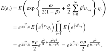
We also have,

Thus

for ρ ≠ 0 and ∣β ∣ < 1.
- 12.5 The estimated models on the return series {r
t
, t = 2, …, 2122} and {r
t
, t = 2123, …, 4245} have the volatilities

Denote by θ (1) = (0.098, 0.087, 0.84)′ and θ (2) = (0.012, 0.075, 0.919)′ the parameters of the two models. The estimated values of ω and β seem quite different. Denote by
 and
and  the estimated standard deviations of the estimators of
ω
and
β
of Model
Mi
. It turns out that the confidence intervals
the estimated standard deviations of the estimators of
ω
and
β
of Model
Mi
. It turns out that the confidence intervals
and

have empty intersection. The same holds true for the confidence intervals

and

The third graph of Figure E.4 displays the boxplot of the distribution of
 on 100 independent simulations of Model M1. The difference
θ
(2) − θ
(1)
between the parameters of M1 and M2 is marked by a diamond shape. The difference
θ
(2) − θ
(1)
is an outlier for the distribution of
on 100 independent simulations of Model M1. The difference
θ
(2) − θ
(1)
between the parameters of M1 and M2 is marked by a diamond shape. The difference
θ
(2) − θ
(1)
is an outlier for the distribution of  , meaning that estimated GARCH on the two periods are significantly distinct.
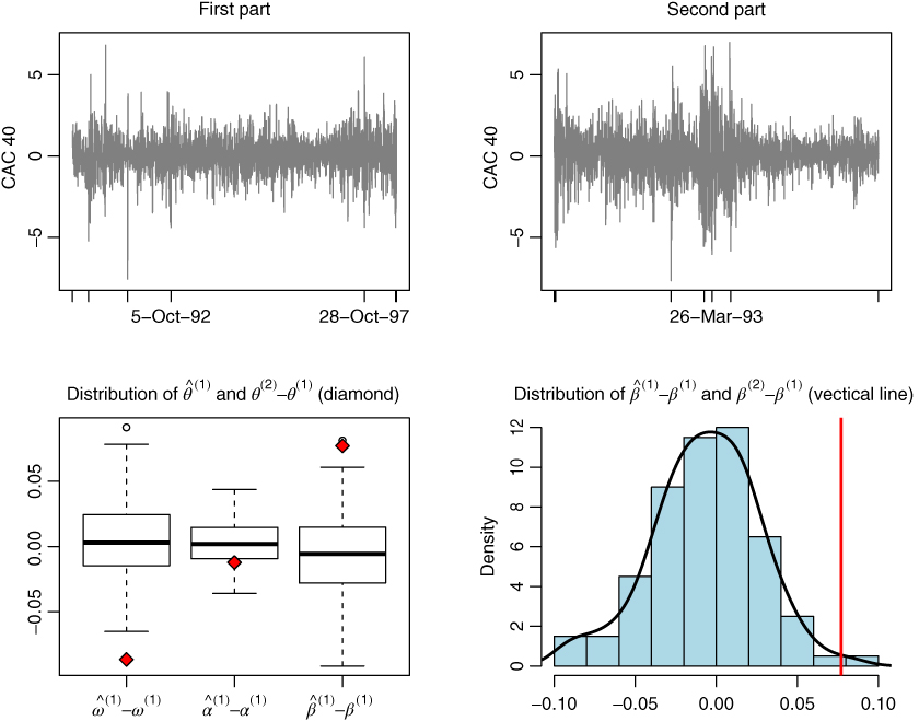
Figure E.4 The parameter θ (1) (respectively, θ (2) ) is that of a GARCH(1,1) fitted on the CAC 40 returns from March 1, 1990 to September 3, 1998 (respectively, from September 4, 1998 to December 29, 2006). The box plots display the empirical distributions of the estimated parameters
 on 100 simulations of the model fitted on the first part of the CAC.
 - 12.6
 is a Markov chain, whose initial probability distribution is given by:
  , and whose transition matrix is:(E.17)
The number of balls in urn
 changes successively from odd to even, and conversely, along the steps. For instance
  . Thus the chain is irreducible but periodic.
Using the formula
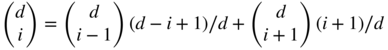 , it can be seen that
  is an invariant law. It follows that
  for all
  .
.When the initial distribution is the Dirac mass at 0 we have
 when
when  is odd, and
  when
when  is even. Thus
  does not exist.
 - 12.7 Let
i
and
j
be two different states, and let
d(i) be the period of state
i
. If the chain is irreducible, there exists an integer
m
1
such that
 and
m
2
such that
and
m
2
such that  . The integer
d(i) divides
m
1 + m
2
since
. The integer
d(i) divides
m
1 + m
2
since  . Similarly
d(i) divides
m
1 + m + m
2
for all
m ∈ {m : p
(m)(j, j) > 0}. Using
m = m + m
1 + m
2 − (m
1 + m
2) = k
1
d(i) − k
2
d(i) = (k
1 − k
2)d(i), it follows that
d(i) divides
m
for all
m ∈ {m : p
(m)(j, j) > 0}. Since
d(j) is the gcd of {m : p
(m)(j, j) > 0}, and we have just shown that
d(i) is a common divisor of all the elements of this set, it follows that
d(i) ≤ d(j). By symmetry, we also have
d(j) ≤ d(i).
. Similarly
d(i) divides
m
1 + m + m
2
for all
m ∈ {m : p
(m)(j, j) > 0}. Using
m = m + m
1 + m
2 − (m
1 + m
2) = k
1
d(i) − k
2
d(i) = (k
1 − k
2)d(i), it follows that
d(i) divides
m
for all
m ∈ {m : p
(m)(j, j) > 0}. Since
d(j) is the gcd of {m : p
(m)(j, j) > 0}, and we have just shown that
d(i) is a common divisor of all the elements of this set, it follows that
d(i) ≤ d(j). By symmetry, we also have
d(j) ≤ d(i).
- 12.8 The key part of the code is the following:
# one iteration of the EM algorithmEM <- function(omega,pi0,p,y){d<-length(omega)n <- length(y) # y contient les n observationsvrais<-0pit.t<-matrix(0,nrow=d,ncol=n)pit.tm1<-matrix(0,nrow=d,ncol=n+1)vecphi<-rep(0,d)pit.tm1[,1]<-pi0for (t in 1:n) {for (j in 1:d) vecphi[j]<-{dnorm(y[t],mean=0,sd=sqrt(abs(omega[j])))}den<-sum(pit.tm1[,t]*vecphi)if(den<=0)return(Inf)pit.t[,t]<-(pit.tm1[,t]*vecphi)/denpit.tm1[,t+1]<-t(p)%*%pit.t[,t]vrais<-vrais+log(den)}pit.n<-matrix(0,nrow=d,ncol=n)pit.n[,n]=pit.t[,n]for (t in n:2) {for (i in 1:d) {pit.n[i,t-1]<- {pit.t[i,t-1]*sum(p[i,1:d]*pit.n[1:d,t]/pit.tm1[1:d,t])}} }pitm1et.n<-array(0,dim=c(d,d,n))for (t in 2:n) {for (i in 1:d) {for (j in 1:d) {pitm1et.n[i,j,t]<-p[i,j]*pit.t[i,t-1]*pit.n[j,t]/pit.tm1[j,t]} } }omega.final<-omegapi0.final<-pi0p.final<-pfor (i in 1:d) {omega.final[i]<-sum((y[1:n]∧2)*pit.n[i,1:n])/sum(pit.n[i,1:n])pi0.final[i]<-pit.n[i,1]for (j in 1:d) {p.final[i,j]<-sum(pitm1et.n[i,j,2:n])/sum(pit.n[i,1:(n-1)])} }liss<-{list(probaliss=pit.n,probatransliss=pitm1et.n,vrais=vrais,omega.final=omega.final,pi0.final=pi0.final,p.final=p.final)}} - 12.9 The last equality of Step 2 of the EM algoritm shows that π t − 1, t ∣ n (i 0, j 0) = 0 for all t . Point 3, then shows that p(i 0, j 0) ≡ 0 in all the subsequent steps of the algorithm.
- 12.10 We have the Markovian representation
 , with
The proof of Theorem 2.4 in Chapter 2 applies directly with this sequence (A t ), showing that there exists a strictly stationary solution if and only if the top Lyapunov exponent of (A t ) is strictly negative. The solution is then unique, non‐anticipative, and ergodic, and takes the form (2.18).
- 12.11 As in Example 2.1, the last exercise shows that the necessary and sufficient strict stationarity condition is

In the ARCH(1) case with d regimes, we obtain the necessary and sufficient condition
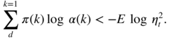
- 12.12 If (ε
t
) is a strictly stationary and non‐anticipative
3
solution and if the sequence (Δ
t
) is iid, then
α(Δ
t
) and
β(Δ
t
) are independent of
 and
and  . If in addition
  then, setting
  , we have
For the existence of a positive solution to this equation, it is necessary to have

Conversely, under this condition, the process

is a strictly stationary and non‐anticipative solution which satisfies
- 12.13 Using the elementary inequality log x ≤ x − 1, we have

and the result follows.
- 12.14 Conditional to the initial variables
 , Equations (12.25), (12.22)–(12.23), (12.26)–(12.28), and (12.29)–(12.31) remain valid, provided the density
φ
k
(ε
t
) is replaced by the density
φ
k
(ε
t
∣ ε
t − 1, …, ε
t − q
) of the Gaussian
, Equations (12.25), (12.22)–(12.23), (12.26)–(12.28), and (12.29)–(12.31) remain valid, provided the density
φ
k
(ε
t
) is replaced by the density
φ
k
(ε
t
∣ ε
t − 1, …, ε
t − q
) of the Gaussian  distribution (and by replacing the notation
M(ε
t
) by
M(ε
t
∣ ε
t − 1, …, ε
t − q
)).
distribution (and by replacing the notation
M(ε
t
) by
M(ε
t
∣ ε
t − 1, …, ε
t − q
)).The EM algorithm cannot be generalised trivially because the maximisation of Eq. (12.32) is replaced by that of

which does not admit an explicit form like (12.35) but requires the use of an optimisation algorithm.
- 12.15 For the MS‐GARCH(1,1) model
 , with
we have

under conditions entailing the existence of the series. For the alternative model, ε t = σ t (Δ t )η t with

we have

Let ℱ t be the sigma‐field generated by the past observations {ε u , u < t}, and by the past and present value of the chain {Δ u , u ≤ t}. We have

but, given the past observations,
 only depends on Δ
t
, whereas
h
t
depends also on {Δ
u
, u < t}.
only depends on Δ
t
, whereas
h
t
depends also on {Δ
u
, u < t}.This entails differences between the two models, in terms of probabilistic properties (the stationarity conditions are easier to obtain for the standard MS‐GARCH model, but they have also been obtained by Liu (2006) for the alternative model), of statistical inference (the fact that
 only depends on Δ
t
renders the alternative model much easier to estimate), and also on the dynamics behaviour and on the interpretation of the parameters.
only depends on Δ
t
renders the alternative model much easier to estimate), and also on the dynamics behaviour and on the interpretation of the parameters.For instance, for the MS‐GARCH, β(i) can be interpreted as a parameter of inertia of the volatility in regime i : if the volatility h t − 1 is high and β(i) is close to 1, the next volatility h t will remain high in regime i . This interpretation is no more valid for the alternative model, since
 may not be equal to
  .
.