4
Alternative Models for the Conditional Variance
Classical GARCH models rely on modelling the conditional variance as a linear function of the squared past innovations. The merits of this specification are its ability to reproduce several important characteristics of financial time series – succession of quiet and turbulent periods, autocorrelation of the squares but absence of autocorrelation of the returns, leptokurticity of the marginal distributions – and the fact that it is sufficiently simple to allow for an extended study of the probability and statistical properties.
The particular functional form of the standard GARCH volatility entails, however, important restrictions. For example, it entails positive autocorrelations of the squares at any lags (see Proposition 2.2). As will see in Part II of this book, the positivity constraints on the GARCH coefficients entail also technical difficulties for the inference. The standard GARCH formulation also does not permit to incorporate exogenous information coming from other time series, for instance macro‐economic variables or intraday realised volatilities, possibly observed at different frequencies.
From an empirical point of view, the symmetric form of the classical GARCH model is one of its most obvious drawbacks. Indeed, by construction, the conditional variance only depends on the modulus of the past variables: past positive and negative innovations have the same effect on the current volatility. This property is in contradiction to many empirical studies on series of stocks, showing a negative correlation between the squared current innovation and the past innovations: if the conditional distribution was symmetric in the past variables, such a correlation would be equal to zero. However, conditional asymmetry is a stylised fact: the volatility increase due to a price decrease is generally stronger than that resulting from a price increase of the same magnitude.
The symmetry property of standard GARCH models has the following interpretation in terms of autocorrelations. If the law of η t is symmetric, and under the assumption that the GARCH process is second‐order stationary, we have
because σ t is an even function of the ε t − i , i > 0 (see Exercise 4.1). Introducing the positive and negative components of ε t ,
it is easily seen that Eq. (4.1) holds if and only if
This characterisation of the symmetry property in terms of autocovariances can be easily tested empirically and is often rejected on financial series. As an example, for the log‐returns series ( ε t = ln(p t /p t − 1)) of the CAC 40 index presented in Chapter 1, we get the results shown in Table 4.1.
Table 4.1 Empirical autocorrelations (CAC 40 series, period 1988–1998).
| h | 1 | 2 | 3 | 4 | 5 | 10 | 20 | 40 |
| ρ(ε t , ε t − h ) | 0.030 | 0.005 | −0.032 | 0.028 | −0.046 a | 0.016 | 0.003 | −0.019 |
| ρ(∣ε t ∣ , ∣ ε t − h ∣) | 0.090 a | 0.100 a | 0.118 a | 0.099 a | 0.086 a | 0.118 a | 0.055 a | 0.032 |
|
|
0.011 | −0.094 a | −0.148 a | −0.018 | −0.127 a | −0.039 a | −0.026 | −0.064 a |
* Autocorrelations which are statistically significant at the 5% level, using 1/n as an approximation of the autocorrelations variances, for n = 2385.
The absence of significant autocorrelations of the returns and the correlation of their modulus or squares, which constitute the basic properties motivating the introduction of GARCH models, is clearly shown for these data. But just as evident is the existence of an asymmetry in the impact of past innovations on the current volatility. More precisely, admitting that the process (ε t ) is second‐order stationary and can be decomposed as ε t = σ t η t , where (η t ) is an iid sequence and σ t is a measurable, positive function of the past of ε t , we have
where
K > 0. For the CAC data, except when
h = 1 for which the autocorrelation is not significant, the estimates of ![]() seem to be significantly negative.
1
Thus
seem to be significantly negative.
1
Thus
which can be interpreted as a higher impact of the past price decreases on the current volatility, compared to the past price increases of the same magnitude. This phenomenon, Cov(σ t , ε t − h ) < 0, is known in the finance literature as the leverage effect 2 : volatility tends to increase dramatically following bad news (that is, a fall in prices), and to increase moderately (or even to diminish) following good news.
The models we will consider in this chapter aim at circumventing some of the above‐mentioned limitations of the standard GARCH models. We start by studying a general class of Stochastic Recurrence Equations (SRE) satisfied by the volatility of most first‐order GARCH formulations.
4.1 Stochastic Recurrence Equation (SRE)
We have seen that the volatility σ t of the standard GARCH(1,1) model ε t = σ t η t satisfies the SRE
This particular SRE can be iterated quite explicitly, and this was used to derive the strictly stationary solution in closed form (see the proof of Theorem 2.1). In this chapter, we consider volatility models satisfying other SREs of the form ![]() In this section, we begin by stating a general result that will be useful to obtain conditions for the existence of a stationary solution of the form
In this section, we begin by stating a general result that will be useful to obtain conditions for the existence of a stationary solution of the form ![]() and for the invertibility of the volatility filter, i.e. the possibility to write the volatility
and for the invertibility of the volatility filter, i.e. the possibility to write the volatility ![]() as a function of the past observations.
as a function of the past observations.
Let E and F be two closed intervals of ℝ, let (X t ) t ∈ ℤ be a stationary and ergodic process valued in E , and let g : E × F → F a function such that y ↦ g(x, y) is Lipschitz continuous for all x ∈ E . Set

The following result can be seen as a particular case of a much more general theory developed in Bougerol (1993) and Straumann and Mikosch (2006).
4.2 Exponential GARCH Model
The following definition for the EGARCH model mimics that given for the strong GARCH.
Stationarity and Existence of Moments
As we have seen, specifications of the function g(·) that are different from (4.10) are possible, depending on the kind of empirical properties we are trying to mimic. The following result does not depend on the specification chosen for g(·). It is, however, assumed that Eg(η t ) exists and is equal to 0.
The previous computation shows that in the Gaussian case, moments exist at any order. This shows that the leptokurticity property may be more difficult to capture with EGARCH than with standard GARCH models.
Assuming that ![]() , the autocorrelation structure of the process
, the autocorrelation structure of the process ![]() can be derived by taking advantage of the ARMA form of the dynamics of
can be derived by taking advantage of the ARMA form of the dynamics of ![]() . Indeed, replacing the terms in
. Indeed, replacing the terms in ![]() by
by ![]() , we get
, we get

Let

One can easily verify that (![]() ) has finite variance. Since
) has finite variance. Since ![]() only depends on a finite number
r
(
r = max(p, q)) of past values of
η
t
, it is clear that Cov(
only depends on a finite number
r
(
r = max(p, q)) of past values of
η
t
, it is clear that Cov(![]() ,
, ![]() ) = 0 for
k > r
. It follows that (
) = 0 for
k > r
. It follows that (![]() ) is an MA(r) process (with intercept) and thus that
) is an MA(r) process (with intercept) and thus that ![]() is an ARMA(p, r) process. This result is analogous to that obtained for the classical GARCH models, for which an ARMA(r, p) representation was exhibited for
is an ARMA(p, r) process. This result is analogous to that obtained for the classical GARCH models, for which an ARMA(r, p) representation was exhibited for ![]() . Apart from the inversion of the integers
r
and
p
, it is important to note that the noise of the ARMA equation of a GARCH is the strong innovation of the square, whereas the noise involved in the ARMA equation of an EGARCH is generally not the strong innovation of
. Apart from the inversion of the integers
r
and
p
, it is important to note that the noise of the ARMA equation of a GARCH is the strong innovation of the square, whereas the noise involved in the ARMA equation of an EGARCH is generally not the strong innovation of ![]() . Under this limitation, the ARMA representation can be used to identify the orders
p
and
q
and to estimate the parameters
β
j
and
α
i
(although the latter do not explicitly appear in the representation).
. Under this limitation, the ARMA representation can be used to identify the orders
p
and
q
and to estimate the parameters
β
j
and
α
i
(although the latter do not explicitly appear in the representation).
The autocorrelations of ![]() can be obtained from formula (4.13). Provided the moments exist we have, for
h > 0,
can be obtained from formula (4.13). Provided the moments exist we have, for
h > 0,

the first product being replaced by 1 if h = 1. For h > 0, this leads to
Invertibility
The existence of a stationary solution (ε t ) to a time series model is often obtained by showing that, for some white noise (η t ) and some measurable function ψ ,
The model is said to be invertible if the reverse holds true, i.e. if
for some measurable function φ .
Under the stationarity condition given in Theorem 4.1, the model ( 4.9) expresses ![]() as a function of the unobserved innovations {η
u
, u < t}. To use the EGARCH model in practice (for instance for predicting
as a function of the unobserved innovations {η
u
, u < t}. To use the EGARCH model in practice (for instance for predicting ![]() by a function of {ε
u
, u < t}), it is necessary to be able to express
by a function of {ε
u
, u < t}), it is necessary to be able to express ![]() as a function of the past observations. Take the example of the EGARCH(1,1) model, which can be rewritten as
as a function of the past observations. Take the example of the EGARCH(1,1) model, which can be rewritten as

Replacing
η
t
by ![]() , one can see that the EGARCH(1,1) satisfies the SRE
, one can see that the EGARCH(1,1) satisfies the SRE
We will thus apply Lemma 4.1. Assuming
β ∈ [0, 1) and −ς < θ < ς
, which appear as reasonable restrictions for the applications (see 2. of Remark 4.3), ![]() belongs to the interval
F = [ω/(1 − β), ∞). We also have
θx + ς ∣ x ∣ ≥ 0 and
belongs to the interval
F = [ω/(1 − β), ∞). We also have
θx + ς ∣ x ∣ ≥ 0 and

Lemma 4.1 then entails the following result, due to Straumann and Mikosch (2006).
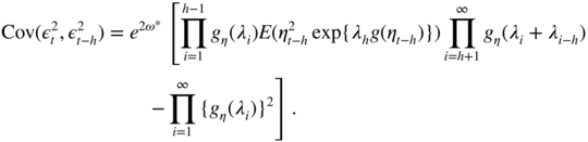
To illustrate the importance of the invertibility issue, consider the EGARCH(1,1) model ( 4.15), with
η
t
iid ![]() and two parameter sets:
and two parameter sets:

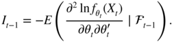
The two models are stationary because ∣β ∣ < 1. Figure 4.1 shows that, for Design A (a), the initial value required for computing recursively the approximation of the volatility has no effect asymptotically. In that case, the volatility at time
t
, when
t
is large, can be accurately approximated by a function of the available observations
ε
1, …, ε
t − 1
. The situation is dramatically different in Design B (b). The estimate ![]() varies considerably with
h
and may be completely different from
varies considerably with
h
and may be completely different from ![]() (for visibility reasons, we have not been able to represent the more extreme values of
(for visibility reasons, we have not been able to represent the more extreme values of ![]() in the graph), even for large
t
.
in the graph), even for large
t
.
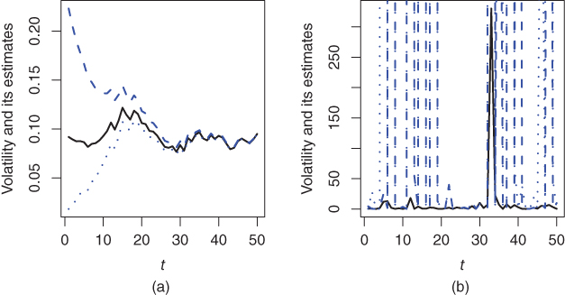
Figure 4.1
Volatility  (in full line) and volatility estimates
  (in dashed and dotted lines) for two different initial values
h
, when the simulated EGARCH model is invertible (Design A, a) or non‐invertible (Design B, b).
(in dashed and dotted lines) for two different initial values
h
, when the simulated EGARCH model is invertible (Design A, a) or non‐invertible (Design B, b).
It must be emphasised that, even if an EGARCH model with parameters as in Design B is a stationary and ergodic process, it cannot be used to recover the volatility from the past observations. In this case, such a model is not very useful. In practice, when an EGARCH is fitted on a real series, it is thus important to assess if the estimated model corresponds to an invertible model (for instance by evaluating the left‐hand side of Eq. (4.16) using Monte Carlo simulations, and/or by studying how ![]() varies with
t
and
h
). The invertibility is also crucial to be able to consistently estimate the parameter of an EGARCH (see Wintenberger 2013).
varies with
t
and
h
). The invertibility is also crucial to be able to consistently estimate the parameter of an EGARCH (see Wintenberger 2013).
4.3 Log‐GARCH Model
A formulation which, at first sight, seems very close to the EGARCH is the Log‐GARCH, initially defined as follows.
To cope with the last two points, one can consider the following asymmetric extension of the Log‐GARCH, which nests the standard Log‐GARCH as a special case.
4.3.1 Stationarity of the Extended Log‐GARCH Model
First consider the case p = q = 1, which can be handled more explicitly than the general case. Write ω − , α + , α − , and β instead of ω 1− , α 1+ , α 1− , and β 1 . The volatility of the model can be rewritten as

Assume that
and
where π + = P(η 0 > 0), π − = P(η 0 < 0), and π 0 = P(η 0 = 0). Recall that, in our notations, we make the convention that 0 × ln x = 0 even if x = 0. Therefore, the case P(η t = 0) > 0 is not precluded by Eq. (4.19). Let
and ![]() defined by
defined by

By the Cauchy rule, the series (4.21) converges absolutely with probability one because
under (4.20), and

The last inequality comes from the fact that ![]() (see Exercise 4.12), which is implied by ( 4.19). Now note that the process
ε
t
= σ
t
η
t
, where
(see Exercise 4.12), which is implied by ( 4.19). Now note that the process
ε
t
= σ
t
η
t
, where ![]() is defined by Eq. ( 4.21) is an extended Log‐GARCH(1,1) process of the form ( 4.18), because {ε
t
= 0} iff {η
t
= 0} and {ε
t
> 0} iff {η
t
> 0}.
is defined by Eq. ( 4.21) is an extended Log‐GARCH(1,1) process of the form ( 4.18), because {ε
t
= 0} iff {η
t
= 0} and {ε
t
> 0} iff {η
t
> 0}.
Now consider the general extended Log‐GARCH( p, q ) process. Because coefficients equal to zero can always be added, it is not restrictive to assume p > 1 and q > 1. Let the vectors
and the matrix

where I k denote the k × k identity matrix. Model ( 4.18) is rewritten in matrix form as
Let γ be the top Lyapunov exponent of the sequence { C t , t ∈ ℤ},
4.3.2 Existence of Moments and Log‐Moments
In Corollary 2.3, we have seen that for the GARCH models, the strict stationarity condition entails the existence of a moment of order
s > 0 for ∣ε
t
∣. The following Lemma shows that this is also the case for ![]() in the Log‐GARCH model, when the condition ( 4.19) is slightly reinforced.
in the Log‐GARCH model, when the condition ( 4.19) is slightly reinforced.
We now give conditions for the existence of higher‐order log‐moments, restricting ourselves to the Log‐GARCH(1,1) case. We have the Markovian representation
with

Under the conditions ( 4.19) and ( 4.20), Eq. (4.25) admits the solution

The next proposition gives conditions for the existence of ![]() and
and ![]() for
m ≥ 1.
for
m ≥ 1.
In the extended Log‐GARCH(1,1) model with α − > max {0, α +} and ω − ≥ 0, negative returns impact future volatilities more importantly than positive returns of the same magnitude when this magnitude is large (at least larger than 1), but the effect of the sign can be reversed for small returns in absolute value. A measure of the average leverage effect can be defined through the covariance between η t − 1 and the current log‐volatility.
If the covariance (4.28) is negative, the leverage effect is present: past negative innovations tend to increase the log‐volatility, and hence the volatility, more than past positive innovations. The sign of the covariance depends not only on all the GARCH coefficients but also on the innovations distribution. Interestingly, the leverage effect may hold with α + > α − and/or ω − < 0.
To illustrate the moment conditions on
ε
t
, as well as the computation of the autocorrelations of ![]() , let us come back to the standard Log‐GARCH(p, q) model
, let us come back to the standard Log‐GARCH(p, q) model

where (η
t
) is iid ![]() . The process
. The process ![]() thus satisfies
thus satisfies
where ![]() ,
, ![]() ,
r = max {p, q},
α
i
= 0 for
i > q
and
β
i
= 0 for
i > p
. Assuming
,
r = max {p, q},
α
i
= 0 for
i > q
and
β
i
= 0 for
i > p
. Assuming ![]() for all ∣z ∣ ≤ 1, we have
for all ∣z ∣ ≤ 1, we have

with

We thus have

Since ![]() , we have
, we have
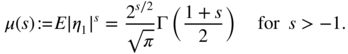
For s ≤ − 1, the moment μ(s) is infinite. This allows to compute

and
for
h ≥ 1. Noting that ln μ(s) = O(s) as
s → 0, these moments exist if and only if
π
i
> − 1/4 for all
i
, which is somewhat a strange moment condition. Another astonishing result is that, if ![]() , then the moment
E|ε
t
|
d
< ∞ if and only if
, then the moment
E|ε
t
|
d
< ∞ if and only if ![]() . If
. If ![]() , then
E|ε
t
|
d
< ∞ for all
d
.
, then
E|ε
t
|
d
< ∞ for all
d
.
Figure 4.2 displays the theoretical autocorrelation function (ACF) of the squares of a Log‐GARCH(2,1) model (4.29) with α 01 = 0.06, β 01 = 1.64, and β 02 = − 0.95. Note the existence of negative autocorrelations. The Log‐GARCH is thus able to take into account lagged countercyclical heteroscedasticity, i.e. the fact that a high volatility period could entail a low volatility period at a certain horizon. According to Proposition 2.2, this is not possible with standard GARCH models.

Figure 4.2 Theoretical autocorrelation function of the squares of a Log‐GARCH(2,1) model.
4.3.3 Relations with the EGARCH Model
Take the example of an EGARCH(1,1) model, which can be written as

where the ![]() 's are iid with
's are iid with ![]() ,
, ![]() , and with the notation
x
+ = max {x, 0} and
x
− = min {x, 0}. The volatility of the EGARCH is given by
, and with the notation
x
+ = max {x, 0} and
x
− = min {x, 0}. The volatility of the EGARCH is given by
Now consider a Log‐GARCH(1,1) of the form

with the parameters
α ≠ 0, ![]() ,
ω
− = − α(c
− − c
+), and the iid sequence
,
ω
− = − α(c
− − c
+), and the iid sequence
with constants c + and c − to be chosen later. The volatility of this Log‐GARCH is given by

Note that, although the processes (ε
t
) and ![]() are not the same, the volatility of the Log‐GARCH is equal to the volatility of the EGARCH. In other words, the class of the Extended Log‐GARCH volatilities includes that of the EGARCH volatilities, and it can be shown that the inclusion is strict (see Figure 4.3).
are not the same, the volatility of the Log‐GARCH is equal to the volatility of the EGARCH. In other words, the class of the Extended Log‐GARCH volatilities includes that of the EGARCH volatilities, and it can be shown that the inclusion is strict (see Figure 4.3).

Figure 4.3 The set of the Extended Log‐GARCH volatilities contains the set of the EGARCH volatilities.
More precisely, we have the following result.
This proposition shows that the class of the Log‐GARCH models generates a richer class of volatilities than the EGARCH.
4.4 Threshold GARCH Model
A natural way to introduce asymmetry is to specify the conditional variance as a function of the positive and negative parts of the past innovations. Recall that
and note that ![]() . The threshold GARCH (TGARCH) class of models introduces a threshold effect into the volatility.
. The threshold GARCH (TGARCH) class of models introduces a threshold effect into the volatility.
Figure 4.4 depicts the major difference between GARCH and TGARCH models. The so‐called ‘news impact curves’ display the impact of the innovations at time t − 1 on the volatility at time t , for first‐order models. In this figure, the coefficients have been chosen in such a way that the marginal variances of ε t in the two models coincide. In this TARCH example, in accordance with the properties of financial time series, negative past values of ε t − 1 have more impact on the volatility than positive values of the same magnitude. The impact is, of course, symmetrical in the ARCH case.

Figure 4.4
News impact curves for the ARCH(1) model,  (dashed line), and the TARCH(1) model,
  (solid line).
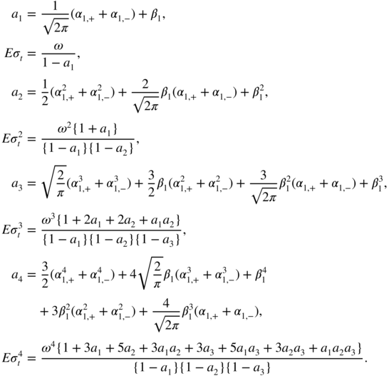
TGARCH models display linearity properties similar to those encountered for the GARCH. Under the positivity constraints (4.34), we have
which allows us to write the conditional standard deviation in the form

where a i (z) = α i, + z + − α i, − z − + β i , i = 1, …, max {p, q}. The dynamics of σ t is thus given by a random coefficient autoregressive model.
Stationarity of the TGARCH(1, 1) Model
The study of the stationarity properties of the TGARCH(1, 1) model is based on Eq. (4.36) and follows from similar arguments to the GARCH(1, 1) case. The strict stationarity condition is written as
In particular, for the TARCH(1) model ( β 1 = 0), we have
Hence, if the distribution of (η t ) is symmetric, the expectation of the two indicator variables is equal to 1/2 and the strict stationarity condition reduces to
Exercise 4.8 shows that the second‐order stationarity condition is
This condition can be made explicit in terms of the first two moments of ![]() and
and ![]() . For instance, if
η
t
is
. For instance, if
η
t
is ![]() distributed, we get
distributed, we get

Of course, the second‐order stationarity condition is more restrictive than the strict stationarity condition (see Figure 4.5).

Figure 4.5
Stationarity regions for the TARCH(1) model with  : 1, second‐order stationarity; 1 and 2, strict stationarity; 3, non‐stationarity.
Under the second‐order stationarity condition, it is easily seen that the property of symmetry ( 4.1) is generally violated. For instance if the distribution of η t is symmetric, we have, for the TARCH(1) model:
whenever α 1, + ≠ α 1, − .
Strict Stationarity of the TGARCH(p, q) Model
The study of the general case relies on a representation analogous to Eq. (2.16), obtained by replacing, in the vector ![]() , the variables
, the variables ![]() by
by ![]() , the
, the ![]() by
σ
t − i
, and by an adequate modification of
by
σ
t − i
, and by an adequate modification of ![]() and
A
t
. Specifically, using (4.35), we get
and
A
t
. Specifically, using (4.35), we get
where

and

is a matrix of size (p + 2q) × (p + 2q),

The following result is analogous to that obtained for the strict stationarity of the GARCH(p, q).
Numerical evaluation, by means of simulation, of the Lyapunov coefficient γ can be time‐consuming because of the large size of the matrices A t . A condition involving matrices of smaller dimensions can sometimes be obtained. Suppose that the asymmetric effects have a factorisation of the form α i− = θα i+ for all lags i = 1, …, q . In this constrained model, the asymmetry is summarised by only one parameter θ ≠ 1, the case θ > 1 giving more importance to the negative returns.
mth‐Order Stationarity of the TGARCH(p, q) Model
Contrary to the standard GARCH model, the odd‐order moments are not more difficult to obtain than the even‐order ones for a TGARCH model. The existence condition for such moments is provided by the following theorem.
The proof of this theorem is identical to that of Theorem 2.9.
Kurtosis of the TGARCH(1, 1) Model
For the TGARCH(1, 1) model with positive coefficients, the condition for the existence of E|ε t | m can be obtained directly. Using the representation
we find that ![]() exists and satisfies
exists and satisfies

if and only if
If this condition is satisfied for
m = 4, then the kurtosis coefficient exists. Moreover, if ![]() , we get
, we get

and, using the notation a i = Ea i (η t ), the moments can be computed successively as
Many moments of the TGARCH(1, 1) can be obtained similarly, such as the autocorrelations of the absolute values (Exercise 4.9) and squares, but the calculations can be tedious.
4.5 Asymmetric Power GARCH Model
The following class is very general and contains the standard GARCH, the TGARCH, and the Log‐GARCH.
Noting that {ε t − i > 0} = {η t − i > 0}, one can write

where

for i = 1, …, max {p, q}.
Stationarity of the APARCH(1, 1) Model
Relation (4.47) is an extension of (2.6) which allows us to obtain the stationarity conditions, as in the classical GARCH(1, 1) case. The necessary and sufficient strict stationarity condition is thus
For the APARCH(1, 0) model, we have

showing that, if the distribution of (η t ) symmetric, the strict stationarity condition reduces to
Note that in the limit case where ∣ς 1 ∣ = 1, the model is strictly stationary for any value of α 1 , as might be expected. Under condition (4.48), the strictly stationary solution is given by
Assuming
E|η
t
|
δ
< ∞, the condition for the existence of ![]() (and of
(and of ![]() ) is
) is
which reduces to
when the distribution of (η t ) symmetric, with

when η t is Gaussian (Γ denoting the Euler gamma function). Figure 4.6 shows the strict and second‐order stationarity regions of the APARCH(1, 0) model when η t is Gaussian.

Figure 4.6
Stationarity regions for the APARCH(1,0) model with  : 1, second‐order stationarity; 1 and 2, strict stationarity; 3, non‐stationarity.
Obviously, if δ ≥ 2, condition (4.49) is sufficient (but not necessary) for the existence of a strictly stationary and second‐order stationary solution to the APARCH(1, 1) model. If δ ≤ 2, condition ( 4.49) is necessary (but not sufficient) for the existence of a second‐order stationary solution.
4.6 Other Asymmetric GARCH Models
Among other asymmetric GARCH models, which we will not study in detail, let us mention the qualitative threshold ARCH (QTARCH) model, and the quadratic GARCH model (QGARCH or GQARCH). The first‐order model of this class, the QGARCH(1, 1), is defined by
where (η t ) is a strong white noise with unit variance, α ≥ 0 and β ≥ 0.
The condition
is clearly necessary for the existence of a non‐anticipative and second‐order stationary solution. To obtain a sufficient condition, we use the approach of Section 4.1. The QGARCH(1, 1) satisfies the SRE
With the notation of Lemma 4.1 and using (4.51), we have

Lemma 4.1 thus entails the following result.
The second equality in (4.50) cannot be easily expanded because of the presence of ![]() and
ε
t − 1 = σ
t − 1
η
t − 1
. It is, therefore, not possible to obtain an explicit solution as a function of the
η
t − i
.
and
ε
t − 1 = σ
t − 1
η
t − 1
. It is, therefore, not possible to obtain an explicit solution as a function of the
η
t − i
.
Many other asymmetric GARCH models have been introduced. Complex asymmetric responses to past values may be considered. For instance, in the model
asymmetry is only present for large innovations (whose amplitude is larger than the threshold γ ).
4.7 A GARCH Model with Contemporaneous Conditional Asymmetry
A common feature of the GARCH models studied up to now is the decomposition
where σ t is a positive variable and (η t ) is an iid process. The various models differ by the specification of σ t as a measurable function of ε t − i for i > 0. This type of formulation implies several important restrictions:
- (i) The process (ε t ) is a martingale difference.
- (ii) The positive and negative parts of ε t have the same volatility, up to a multiplicative factor.
- (iii) The kurtosis and skewness of the conditional distribution of ε t are constant.
Property (ii) is an immediate consequence of the equalities in ( 4.35). Property (iii) expresses the fact that the conditional law of ε t has the same ‘shape’ (symmetric or asymmetric, unimodal or polymodal, with or without heavy tails) as the law of η t .
It can be shown empirically that these properties are generally not satisfied by financial time series. Estimated kurtosis and skewness coefficients of the conditional distribution often present large variations in time. Moreover, property (i) implies that Cov(ε t , z t − 1) = 0, for any variable z t − 1 ∈ L 2 which is a measurable function of the past of ε t . In particular, one must have
or equivalently,
We emphasise the difference between (4.52) and the characterisation (4.2) of the asymmetry studied previously. When Eq. ( 4.52) does not hold, one can speak of contemporaneous asymmetry since the variables ![]() and
and ![]() , of the current date, do not have the same conditional distribution.
, of the current date, do not have the same conditional distribution.
For the CAC index series, Table 4.2 completes Table 4.1, by providing the cross empirical autocorrelations of the positive and negative parts of the returns.
Table 4.2 Empirical autocorrelations (CAC 40, for the period 1988–1998).
| h | 1 | 2 | 3 | 4 | 5 | 10 | 20 | 40 |
|
|
0.037 | −0.006 | −0.013 | 0.029 | −0.039 a | 0.017 | 0.023 | 0.001 |
|
|
−0.013 | −0.035 | −0.019 | −0.025 | −0.028 | −0.007 | −0.020 | 0.017 |
|
|
0.026 | 0.088 a | 0.135 a | 0.047 a | 0.088 a | 0.056 a | 0.049 a | 0.065 a |
|
|
0.060 a | 0.074 a | 0.041 a | 0.070 a | 0.027 | 0.077 a | 0.015 | −0.008 a |
* Parameters that are statistically significant at the level 5%, using 1/n as an approximation for the autocorrelations variance, for n = 2385.
Without carrying out a formal test, comparison of rows 1 and 3 (or 2 and 4) shows that the leverage effect is present, whereas comparison of rows 3 and 4 shows that property ( 4.28) does not hold.
A class of GARCH‐type models allowing the two kinds of asymmetry is defined as follows. Let
where {η t } is centred, η t is independent of σ t, + and σ t, − , and

where ![]() α
0, +, α
0, − > 0. Without loss of generality, it can be assumed that
α
0, +, α
0, − > 0. Without loss of generality, it can be assumed that ![]() .
.
As an immediate consequence of the positivity of σ t, + and σ t, − , we obtain
which is crucial for the study of this model.
Thus,
σ
t, +
and
σ
t, −
can be interpreted as the volatilities of the positive and negative parts of the noise (up to a multiplicative constant, since we did not specify the variances of ![]() and
and ![]() ). In general, the non‐anticipative solution of this model, when it exists, is not a martingale difference because
). In general, the non‐anticipative solution of this model, when it exists, is not a martingale difference because
An exception is, of course, the situation where the parameters of the dynamics of σ t, + and σ t, − coincide, in which case we obtain model ( 4.33).
A simple computation shows that the kurtosis coefficient of the conditional law of ε t is given by

where ![]() , provided that
, provided that ![]() . A similar computation can be done for the conditional skewness, showing that the shape of the conditional distribution varies in time, in a more important way than for classical GARCH models.
. A similar computation can be done for the conditional skewness, showing that the shape of the conditional distribution varies in time, in a more important way than for classical GARCH models.
Methods analogous to those developed for the other GARCH models allow us to obtain existence conditions for the stationary and non‐anticipative solutions (references are given at the end of the chapter). In contrast to the GARCH models analysed previously, the stationary solution (ε t ) is not always a white noise.
4.8 Empirical Comparisons of Asymmetric GARCH Formulations
We will restrict ourselves to the simplest versions of the GARCH introduced in this chapter and consider their fit to the series of CAC 40 index returns, r t , over the period 1988–1998 consisting of 2385 values.
Descriptive Statistics
Figure 4.7 displays the first 500 values of the series. The volatility clustering phenomenon is clearly evident. The correlograms in Figure 4.8 indicate absence of autocorrelation. However, squared returns present significant autocorrelations, which is another sign that the returns are not independent. Ljung–Box portmanteau tests, such as those available in SAS (see Table 4.3; Chapter 5 gives more details on these tests), confirm the visual analysis provided by the correlograms. Figure 4.9a, compared to Figure 4.8b, seems to indicate that the absolute returns are slightly more strongly correlated than the squares. Figure 4.9b displays empirical correlations between the series ∣r t ∣ and r t − h . It can be seen that these correlations are negative, which implies the presence of leverage effects (more accentuated, apparently, for lags 2 and 3 than for lag 1).

Figure 4.7 The first 500 values of the CAC 40 index (a) and of the squared index (b).

Figure 4.8
Correlograms of the CAC 40 index (a) and the squared index (b). Dashed lines correspond to  .
.
Table 4.3 Portmanteau test of the white noise hypothesis for the CAC 40 series (a) and for the squared index (b).
a: Autocorrelation check for white noise
To Chi‐ Pr >
Lag square DF Khi2 ‐‐‐‐‐‐‐‐‐‐‐‐‐‐‐Autocorrelations‐‐‐‐‐‐‐‐‐‐‐‐‐‐‐
6 11.51 6 0.0737 0.030 0.005 −0.032 0.028 −0.046 −0.001
12 16.99 12 0.1499 −0.018 −0.014 0.034 0.016 0.017 0.010
18 21.22 18 0.2685 −0.005 0.025 −0.031 −0.009 −0.003 0.006
24 27.20 24 0.2954 −0.023 0.003 −0.010 0.030 −0.027 −0.015
b: Autocorrelation check for white noise
To Chi‐ Pr >
Lag square DF Khi2 ‐‐‐‐‐‐‐‐‐‐‐‐‐‐‐Autocorrelations‐‐‐‐‐‐‐‐‐‐‐‐‐‐‐
6 165.90 6 <0.0001 0.129 0.127 0.117 0.084 0.101 0.074
12 222.93 12 <0.0001 0.051 0.060 0.070 0.092 0.058 0.030
18 238.11 18 <0.0001 0.053 0.036 0.020 0.041 0.002 0.013
24 240.04 24 <0.0001 0.006 0.024 0.013 0.003 0.001 −0.002
|

Figure 4.9
Correlogram  of the absolute CAC 40 returns (a) and cross correlograms
  measuring the leverage effects (b).
Fit by Symmetric and Asymmetric GARCH Models
We will consider the classical GARCH(1, 1) model and the simplest asymmetric models (which are the most widely used). Using the AUTOREG and MODEL procedures of SAS, the estimated models are
- GARCH(1, 1) model4.57

- EGARCH(1, 1) model4.58

- QGARCH(1, 1) model4.59

- GJR‐GARCH(1, 1) model4.60

- TGARCH(1, 1) model4.61

Interpretation of the Estimated Coefficients
Note that all the estimated models are stationary. The standard GARCH(1, 1) admits a fourth‐order moment since, in view of the computation on p. 45, we have 3α
2 + β
2 + 2αβ < 1. It is thus possible to compute the variance and kurtosis in this estimated model (which are, respectively, equal to 1.3 × 10⁻⁴
and 3.49 for the standard GARCH(1,1)). Given the ARMA(1, 1) representation for ![]() , we have
, we have ![]() for any
h > 1. Since
for any
h > 1. Since ![]() is close to 1, the decay of
is close to 1, the decay of ![]() to zero will be slow when
h → ∞, which can be interpreted as a sign of strong persistence of shocks.
4
to zero will be slow when
h → ∞, which can be interpreted as a sign of strong persistence of shocks.
4
Note that in the EGARCH model the parameter
θ = − 0.53 is negative, implying the presence of the leverage effect. A similar interpretation can be given to the negative sign of the coefficient of
ε
t − 1
in the QGARCH model, and to that of ![]() in the GJR‐GARCH model. In the TGARCH model, the leverage effect is present since
α
1, − > α
1, + > 0.
in the GJR‐GARCH model. In the TGARCH model, the leverage effect is present since
α
1, − > α
1, + > 0.
The TGARCH model seems easier to interpret than the other asymmetric models. The volatility (that is, the conditional standard deviation) is the sum of four terms. The first is the intercept ω = 8 × 10⁻⁴ . The term ω/(1 − β 1) = 0.006 can be interpreted as a ‘minimal volatility’, obtained by assuming that all the innovations are equal to zero. The next two terms represent the impact of the last observation, distinguishing the sign of this observation, on the current volatility. In the estimated model, the impact of a positive value is 3.5 times less than that of a negative one. The last coefficient measures the importance of the last volatility. Even in absence of news, the decay of the volatility is slow because the coefficient β 1 = 0.87 is rather close to 1.
Likelihood Comparisons
Table 4.4 gives the log‐likelihood, ln L n , of the observations for the different models. One cannot directly compare the log‐likelihood of the standard GARCH(1, 1) model, which has one parameter less, with that of the other models, but the log‐likelihoods of the asymmetric models, which all have five parameters, can be compared. The largest likelihood is observed for the GJR threshold model, but, the difference being very slight, it is not clear that this model is really superior to the others.
Table 4.4 Likelihoods of the different models for the CAC 40 series.
| GARCH | EGARCH | QGARCH | GJR‐GARCH | TGARCH | |
| ln L n | 7393 | 7404 | 7404 | 7406 | 7405 |
Resemblances between the Estimated Volatilities
Figure 4.10 shows that the estimated volatilities for the five models are very similar. It follows that the different specifications produce very similar prediction intervals (see Figure 4.11).

Figure 4.10 From left to right and top to bottom, graph of the first 500 values of the CAC 40 index and estimated volatilities (×104 ) for the GARCH(1, 1), EGARCH(1, 1), QGARCH(1, 1), GJR‐GARCH(1, 1), and TGARCH(1, 1) models.
Figure 4.11
Returns
r
t
of the CAC 40 index (solid lines) and confidence intervals  (dotted lines), where
  is the empirical mean of the returns over the whole period 1988–1998 and
σ
t
is the estimated volatility in the standard GARCH(1, 1) model (a) and in the EGARCH(1, 1) model (b).
is the empirical mean of the returns over the whole period 1988–1998 and
σ
t
is the estimated volatility in the standard GARCH(1, 1) model (a) and in the EGARCH(1, 1) model (b).
Distances between Estimated Models
Differences can, however, be discerned between the various specifications. Table 4.5 gives an insight into the distances between the estimated volatilities for the different models. From this point of view, the TGARCH and EGARCH models are very close and are also the most distant from the standard GARCH. The QGARCH model is the closest to the standard GARCH. Rather surprisingly, the TGARCH and GJR‐GARCH models appear quite different. Indeed, the GJR‐GARCH is a threshold model for the conditional variance and the TGARCH is a similar model for the conditional standard deviation.
Table 4.5 Means of the squared differences between the estimated volatilities (×1010 ).
| GARCH | EGARCH | QGARCH | GJR | TGARCH | |
| GARCH | 0 | 10.98 | 3.58 | 7.64 | 12.71 |
| EGARCH | 10.98 | 0 | 3.64 | 6.47 | 1.05 |
| QGARCH | 3.58 | 3.64 | 0 | 3.25 | 4.69 |
| GJR | 7.64 | 6.47 | 3.25 | 0 | 9.03 |
| TGARCH | 12.71 | 1.05 | 4.69 | 9.03 | 0 |
Figure 4.12 confirms the results of Table 4.5. The left‐hand scatterplot shows

Figure 4.12 Comparison of the estimated volatilities of the EGARCH and TARCH models (a), and of the TGARCH and GJR‐GARCH models (b). The estimated volatilities are close when the scatterplot is elongated (see text).
and the right‐hand one
The left‐hand graph shows that the difference between the estimated volatilities of the TGARCH and the standard GARCH, denoted by ![]() , is always very close to the difference between the estimated volatilities of the EGARCH and the standard GARCH, denoted by
, is always very close to the difference between the estimated volatilities of the EGARCH and the standard GARCH, denoted by ![]() (the difference from the standard GARCH is introduced to make the graphs more readable). The right‐hand graph shows much more important differences between the TGARCH and GJR‐GARCH specifications.
(the difference from the standard GARCH is introduced to make the graphs more readable). The right‐hand graph shows much more important differences between the TGARCH and GJR‐GARCH specifications.
Comparison between Implied and Sample Values of the Persistence and of the Leverage Effect
We now wish to compare, for the different models, the theoretical autocorrelations ρ(∣r t ∣ , ∣ r t − h ∣) and ρ(∣r t ∣ , r t − h ) to the empirical ones. The theoretical autocorrelations being difficult – if not impossible – to obtain analytically, we used simulations of the estimated model to approximate these theoretical autocorrelations by their empirical counterparts. The length of the simulations, 50 000, seemed sufficient to obtain good accuracy (this was confirmed by comparing the empirical and theoretical values when the latter were available).
Figure 4.13 shows satisfactory results for the standard GARCH model, as far as the autocorrelations of absolute values are concerned. Of course, this model is not able to reproduce the correlations induced by the leverage effect. Such autocorrelations are adequately reproduced by the TGARCH model, as can be seen from the top and bottom right panels. The autocorrelations for the other asymmetric models are not reproduced here but are very similar to those of the TGARCH. The negative correlations between r t and the r t − h appear similar to the empirical ones.

Figure 4.13 Correlogram h ↦ ρ(∣r t ∣ , ∣ r t − h ∣) of the absolute values (left) and cross correlogram h ↦ ρ(∣r t ∣ , r t − h ) measuring the leverage effect (right), for the CAC 40 series (top), for the standard GARCH (middle), and for the TGARCH (bottom) estimated on the CAC 40 series.
Implied and Empirical Kurtosis
Table 4.6 shows that the theoretical variances obtained from the estimated models are close to the observed variance of the CAC 40 index. In contrast, the estimated kurtosis values are all much below the observed value.
Table 4.6 Variance (×104 ) and kurtosis of the CAC 40 index and of simulations of length 50 000 of the five estimated models.
| CAC 40 | GARCH | EGARCH | QGARCH | GJR | TGARCH | |
| Kurtosis | 5.9 | 3.5 | 3.4 | 3.3 | 3.6 | 3.4 |
| Variance | 1.3 | 1.3 | 1.3 | 1.3 | 1.3 | 1.3 |
In all these five models, the conditional distribution of the returns is assumed to be ![]() . This choice may be inadequate, which could explain the discrepancy between the estimated theoretical and the empirical kurtosis. Moreover, the normality assumption is clearly rejected by statistical tests, such as the Kolmogorov–Smirnov test, applied to the standardised returns. A leptokurtic distribution is observed for those standardised returns.
. This choice may be inadequate, which could explain the discrepancy between the estimated theoretical and the empirical kurtosis. Moreover, the normality assumption is clearly rejected by statistical tests, such as the Kolmogorov–Smirnov test, applied to the standardised returns. A leptokurtic distribution is observed for those standardised returns.
Table 4.7 reveals a large number of returns outside the interval ![]() , whatever the specification used for
, whatever the specification used for ![]() . If the conditional law were Gaussian and if the conditional variance were correctly specified, the probability of one return falling outside the interval would be 2{1 − Φ(3)} = 0.0027, which would correspond to an average of 6 values out of 2385.
. If the conditional law were Gaussian and if the conditional variance were correctly specified, the probability of one return falling outside the interval would be 2{1 − Φ(3)} = 0.0027, which would correspond to an average of 6 values out of 2385.
Table 4.7
Number of CAC returns outside the limits ![]() (THEO being the theoretical number when the conditional distribution is
(THEO being the theoretical number when the conditional distribution is ![]() .
.
| THEO | GARCH | EGARCH | QGARCH | GJR | TGARCH |
| 6 | 17 | 13 | 14 | 15 | 13 |
Asymmetric GARCH Models with Non‐Gaussian Innovations
To take into account the leptokurtic shape of the residuals distribution, we re‐estimated the five GARCH models with a Student t distribution – whose parameter is estimated – for η t .
For instance, the new estimated TGARCH model is

It can be seen that the estimated volatility is quite different from that obtained with the normal distribution (see Table 4.8).
Table 4.8 Means of the squares of the differences between the estimated volatilities (×1010 ) for the models with Student innovations and the TGARCH model with Gaussian innovations (model ( 4.33) denoted TGARCH N ).
| GARCH | EGARCH | QGARCH | GJR | TGARCH | TGARCH N | |
| GARCH | 0 | 5.90 | 2.72 | 5.89 | 7.71 | 15.77 |
| EGARCH | 5.90 | 0 | 2.27 | 5.08 | 0.89 | 8.92 |
| QGARCH | 2.72 | 2.27 | 0 | 2.34 | 3.35 | 9.64 |
| GJR | 5.89 | 5.08 | 2.34 | 0 | 7.21 | 11.46 |
| TGARCH | 7.71 | 0.89 | 3.35 | 7.21 | 0 | 7.75 |
| TGARCH N | 15.77 | 8.92 | 9.64 | 11.46 | 7.75 | 0 |
Model with Interventions
Analysis of the residuals show that the values observed at times t = 228, 682, and 845 are scarcely compatible with the selected model. There are two ways to address this issue: one could either research a new specification that makes those values compatible with the model, or treat these three values as outliers for the selected model.
In the first case, one could replace the ![]() distribution of the noise
η
t
with a more appropriate (leptokurtic) one. The first difficulty with this is that no distribution is evident for these data (it is clear that distributions of Student
t
or generalised error type would not provide good approximations of the distribution of the standardised residuals). The second difficulty is that changing the distribution might considerably enlarge the confidence intervals. Take the example of a 99% confidence interval at horizon 1. The initial interval
distribution of the noise
η
t
with a more appropriate (leptokurtic) one. The first difficulty with this is that no distribution is evident for these data (it is clear that distributions of Student
t
or generalised error type would not provide good approximations of the distribution of the standardised residuals). The second difficulty is that changing the distribution might considerably enlarge the confidence intervals. Take the example of a 99% confidence interval at horizon 1. The initial interval ![]() simply becomes the dilated interval
simply becomes the dilated interval ![]() with
t
0.995 > 2.57, provided that the estimates
with
t
0.995 > 2.57, provided that the estimates ![]() are not much affected by the change of conditional distribution. Even if the new interval does contain 99% of returns, there is a good chance that it will be excessively large for most of the data.
are not much affected by the change of conditional distribution. Even if the new interval does contain 99% of returns, there is a good chance that it will be excessively large for most of the data.
So for this first case, we should ideally change the prediction formula for
σ
t
so that the estimated volatility is larger for the three special data (the resulting smaller standardized residuals ![]() would become consistent with the
would become consistent with the ![]() distribution), without much changing volatilities estimated for other data. Finding a reasonable model that achieves this change seems quite difficult.
distribution), without much changing volatilities estimated for other data. Finding a reasonable model that achieves this change seems quite difficult.
We have, therefore, opted for the second approach, treating these three values as outliers. Conceptually, this amounts to assuming that the model is not appropriate in certain circumstances. One can imagine that exceptional events occurred shortly before the three dates t = 228, 682, and 845. Other special events may occur in the future, and our model will be unable to anticipate the changes in volatility induced by these extraordinary events. The ideal would be to know the values that returns would have had if these exceptional event had not occurred, and to work with these corrected values. This is, of course, not possible, and we must also estimate the adjusted values. We will use an intervention model, assuming that only the returns of the three dates would have changed in the absence of the above‐mentioned exceptional events. Other types of interventions can, of course, be envisaged. To estimate what would have been the returns of the three dates in the absence of exceptional events, we can add these three values to the parameters of the likelihood. This can easily be done using a SAS program (see Table 4.9).
Table 4.9 SAS program for the fitting of a TGARCH(1, 1) model with interventions.
/* Data reading */
data cac;
infile 'c:enseignementPRedessGarchcac8898.dat';
input indice; date=_n_;
run;
/* Estimation of a TGARCH(1,1) model */
proc model data = cac ;
/* Initial values are attributed to the parameters */
parameters cacmod1 ‐0.075735 cacmod2 ‐0.064956
cacmod3 ‐0.0349778 omega .000779460
alpha_plus 0.034732 alpha_moins 0.12200 beta 0.86887
intercept .000426280 ;
/* The index is regressed on a constant and 3 interventions
are made*/
if (_obs_ = 682) then indice= cacmod1;
else if (_obs_ = 228) then indice= cacmod2;
else if (_obs_ = 845) then indice= cacmod3;
else indice = intercept ;
/* The conditional variance is modeled by a TGARCH */
if (_obs_ = 1) then
if((alpha_plus+alpha_moins)/sqrt(2*constant('pi'))+beta=1)
then
h.indice = (omega + (alpha_plus/2+alpha_moins/2+beta)
*sqrt(mse.indice))**2 ;
2else h.indice = (omega/(1‐(alpha_plus+alpha_moins)/
sqrt(2*constant('pi'))‐beta))**2;
else
if zlag(‐resid.indice) > 0 then h.indice = (omega
+ alpha_plus*zlag(‐resid.indice)
+ beta*zlag(sqrt(h.indice)))**2 ;
else h.indice = (omega ‐ alpha_moins*zlag(‐resid.indice)
+ beta*zlag(sqrt(h.indice)))**2 ;
/* The model is fitted and the normalized residuals are
stored in a SAS table*/
outvars nresid.indice;
fit indice / method = marquardt fiml out=residtgarch ;
run ; quit ;
|
4.9 Models Incorporating External Information
GARCH‐X Models
The usual GARCH‐type models predict the squared returns ![]() by means of the past returns only {ε
u
, u < t}. It is, however, often the case that some extra information is available, under the form of a vector
x
t − 1
of exogenous covariates, such as the daily volume of transactions, or high frequency intraday data, or even series of other returns. To take advantage of the extra information – in order to improve the prediction of the squares – GARCH models that are augmented with additional explanatory variables (GARCH‐X models in short), can be considered. A simple version of GARCH‐X is of the form
by means of the past returns only {ε
u
, u < t}. It is, however, often the case that some extra information is available, under the form of a vector
x
t − 1
of exogenous covariates, such as the daily volume of transactions, or high frequency intraday data, or even series of other returns. To take advantage of the extra information – in order to improve the prediction of the squares – GARCH models that are augmented with additional explanatory variables (GARCH‐X models in short), can be considered. A simple version of GARCH‐X is of the form

where x t = (x 1, t , …, x r, t )′ is a vector of r exogenous covariates. The term ‘exogenous’ does not refer to the concepts of weak or strong exogeneity introduced in the econometric literature, but is employed because the dynamics if the vector x t is not specified by the GARCH‐X model (4.63).
To ensure ![]() with probability one, assume that the covariates are a.s. positive and that the coefficients satisfy
α ≥ 0,
β ≥ 0,
ω > 0, and
π
= (π
1, …, π
r
)′ ≥ 0 componentwise. In the GARCH‐type models, the sequence (η
t
) is traditionally assumed to be iid(0, 1), but the assumption is not necessary for the following result.
with probability one, assume that the covariates are a.s. positive and that the coefficients satisfy
α ≥ 0,
β ≥ 0,
ω > 0, and
π
= (π
1, …, π
r
)′ ≥ 0 componentwise. In the GARCH‐type models, the sequence (η
t
) is traditionally assumed to be iid(0, 1), but the assumption is not necessary for the following result.
It is interesting to note that, under Assumption A, the stationarity condition of (ε t ) is not modified by the presence of the exogenous variables. Note that if
where ℱ
t − 1
is the information set generated by {ε
u
,
x
u
: u < t}, then ![]() is the conditional variance of
ε
t
given ℱ
t − 1
.
is the conditional variance of
ε
t
given ℱ
t − 1
.
HEAVY Models
Intraday high‐frequency data, and thus realised volatility measures RM
t
(such as the realized variance), are increasingly available. This extra information can be included as exogenous variable
x
t
= RM
t
in model ( 4.63), which generally greatly improves the prediction of ![]() . The drawback of the GARCH‐X model is however that the dynamics of the covariate is not specified. This forces the practitioner to put in the volatility equation of
. The drawback of the GARCH‐X model is however that the dynamics of the covariate is not specified. This forces the practitioner to put in the volatility equation of ![]() only variables that will be available (or predictable) at time
t + h
, which is restrictive if the horizon of prediction
h
is larger than 1. To specify the dynamics of (RM
t
), Shephard and Sheppard (2010) proposed the high‐frequency‐based volatility (HEAVY) model, in which Model ( 4.63)
only variables that will be available (or predictable) at time
t + h
, which is restrictive if the horizon of prediction
h
is larger than 1. To specify the dynamics of (RM
t
), Shephard and Sheppard (2010) proposed the high‐frequency‐based volatility (HEAVY) model, in which Model ( 4.63)

is completed by the Multiplicative Error Model (MEM)

where (z t ) is a stationary sequence of positive variables such that E(z t |ℱ t − 1) = 1, ω * > 0, α * ≥ 0 and β * ≥ 0.
Realised‐GARCH Models
An alternative model has been proposed by Hansen, Huang, and Shek (2012) (see also Hansen and Huang, 2016). In this model, called realised‐GARCH, a GARCH‐X equation similar to Eq. ( 4.64), or alternatively a Log‐GARCH‐X equation of the form

is completed by a measurement equation for the realised volatility measure, that can take the form
where (u
t
) is a strong white noise independent of (η
t
). Note that the dynamics are written on the logarithm of the volatility and of the realised volatility measure, in order to avoid positivity constraints. The term
τ(η
t
) is assumed to be centred, for instance of the form
τ(z) = τ
1
z + τ
2(z
2 − 1), and can thus take into account the leverage effect. Defining a strong white noise (![]() ) by
) by ![]() = τ(η
t − 1) + u
t − 1, one can see that
= τ(η
t − 1) + u
t − 1, one can see that ![]() satisfies the AR(1) model
satisfies the AR(1) model
from which stationarity conditions follow. Note, however, that the realised‐GARCH is not a stochastic volatility model (see Chapter 12) because ![]() is measurable with respect to the sigma‐field ℱ
t − 1
generated by {RM
u
: u < t}.
is measurable with respect to the sigma‐field ℱ
t − 1
generated by {RM
u
: u < t}.
Intraday Scale Models
Visser (2011) proposed a model that directly links the daily returns and the intraday price movements. Let
p
t
(u) be the price of an asset at the intraday time
u ∈ [0, 1] of the day
t ∈ ℕ. Consider the continuous‐time log‐return process
R
t
(u) = ln p
t
(u)/p
t
(0). Note that the open‐to‐close daily return is
ε
t
= R
t
(1). If, for example,
R
t
(u) = σ
t
W
t
(u) where {W
t
(·)}
t
is an iid sequence of standard Brownian motions, then we have the ARCH‐type equation
ε
t
= σ
t
η
t
where (η
t
) is iid ![]() . In this model, the realised volatility – usually defined as the sum of the squared five‐minute returns – should be a good proxy of the volatility since
. In this model, the realised volatility – usually defined as the sum of the squared five‐minute returns – should be a good proxy of the volatility since

in mean square as h → 0 (see Exercise 4.13). More generally, denoting by D[0, 1] the set of the real‐valued function on [0,1] which are right continuous with left limits (càdlàg), if one assumes
and
that is, H(cR) = cH(R) for all c ≥ 0 and R ∈ D[0, 1], then the realized measure RM t = H(R t (·)) satisfies the ARCH, or more precisely the MEM‐type equation
Noting that ![]() , Visser (2011) showed that, up to the unknown scaling constant
, Visser (2011) showed that, up to the unknown scaling constant ![]() , the parameters giving the dynamics of the daily volatility
σ
t
can also be estimated from a MEM model on the sequence (RM
t
). The resulting estimators are generally more accurate than those based on (ε
t
), intuitively because the variance of RM
t
is often much smaller than that of
, the parameters giving the dynamics of the daily volatility
σ
t
can also be estimated from a MEM model on the sequence (RM
t
). The resulting estimators are generally more accurate than those based on (ε
t
), intuitively because the variance of RM
t
is often much smaller than that of ![]() .
.
MIDAS Models
The previous models aim at explaining a daily variable (the squared returns) by an intraday variable. More generally, MIxed DAta Sampling (MIDAS) regression is a technique that can be used when independent variables appear at higher frequencies than the dependent variable (see Wang and Ghysels (2015) and the references therein). Engle, Ghysels, and Sohn (2013) proposed a GARCH‐MIDAS model with a short‐run volatility component g t and a long‐run volatility component τ t . The short‐run component g t is the volatility of a unit‐variance GARCH(1,1) process, defined by

with
α > 0,
β ≥ 0, and
α + β < 1. As usual, (η
t
) denotes an iid (0,1) sequence. The observed sequence of returns (r
t
) is then assumed to follow an ARCH‐type model with the error term
ε
t
and a volatility
τ
t
driven by past realised volatilities ![]() :
:

The parameters m and θ are positive. The weights ϕ k are positive, and their sum is equal to 1. For instance, one can take

Note that

with ω = m and q = K + N − 1. The first ARCH coefficient is α 1 = θϕ 1 and the last one is α q = θϕ K . Compared to a standard ARCH(q), the error term ε t is not iid(0,1), but is a GARCH(1,1). The stationarity condition remains, however, the same (see e.g. Remark 4.1, or Theorem 4.9 showing that the iid assumption can be replaced by an assumption of the form A).
4.10 Models Based on the Score: GAS and Beta‐t‐(E)GARCH
Assume an iid sample
X
1, …, X
n
of density
f
θ
depending on an unknown parameter
θ ∈ ℝ
d
. It is rarely possible to find analytically the maximum likelihood estimator ![]() maximising the log‐likelihood
maximising the log‐likelihood

Starting from a current approximation
θ
(k)
of ![]() , a Taylor expansion shows that under some regularity conditions
, a Taylor expansion shows that under some regularity conditions
where ![]() is an estimate of the Fisher information matrix and
is an estimate of the Fisher information matrix and ![]() is called the score. Assuming
is called the score. Assuming ![]() invertible, we thus have
invertible, we thus have ![]() which suggests to update the approximation of
which suggests to update the approximation of ![]() by the so‐called Newton–Raphson iteration
by the so‐called Newton–Raphson iteration
Now consider a time series whose conditional distribution is driven by a time‐varying parameter
θ
t
being a measurable function of the sigma‐field ℱ
t − 1
generated by the past values {X
u
, u < t}. Roughly speaking, one can say that the larger ![]() is, the more plausible the time series model (i.e. the time‐varying parameter
θ
t
). If
is, the more plausible the time series model (i.e. the time‐varying parameter
θ
t
). If ![]() is not maximal, the score
is not maximal, the score ![]() is not null, and one may want to improve the ‘likelihood’ of the time series model by updating
θ
t
using an equation based on the score, in the spirit of the Newton–Raphson iteration (4.71). Creal, Koopman, and Lucas (2013) proposed an updating equation of the form
is not null, and one may want to improve the ‘likelihood’ of the time series model by updating
θ
t
using an equation based on the score, in the spirit of the Newton–Raphson iteration (4.71). Creal, Koopman, and Lucas (2013) proposed an updating equation of the form

where S(θ t ) is a scaling factor which may be, similar to Eq. ( 4.71), the inverse of conditional information matrix
The Eqs. (4.72) and (4.73) define a Generalized Autoregressive Score (GAS) model. The parameters ω, α and β involved in (4.73) do not appear in the Newton–Raphson iteration (4.71). An argument for including those parameters can be found in Blasques, Koopman and Lucas (2015).
Take the example of a volatility model
ε
t
= σ
t
η
t
with Gaussian innovations. In this example the time‐varying parameter is ![]() and the conditional distribution of
ε
t
is
and the conditional distribution of
ε
t
is

with
φ
the ![]() density. The score and conditional information are thus
density. The score and conditional information are thus

The updating Eq. ( 4.73) becomes, with ![]() ,
,
which is a standard GARCH(1,1) equation. The updating equation depends drastically on the assumed conditional distribution. Assume, for instance that, instead of a Gaussian, the conditional distribution is a Student with ν > 2 degrees of freedom, normalised to obtain a unit variance. The updating Eq. ( 4.73) becomes

which is the Beta‐t‐GARCH of Harvey and Chakravarty (2008) (see Exercise 4.14).
8
Note that when
ν
is small, an extreme value of ![]() has a lower impact on the volatility (4.75) than on the volatility (4.74), in agreement with the fact that an extreme value is more likely to occur with a Student than with a Gaussian distribution. In some sense, GAS models are motivated by a kind of generalization of the likelihood principle, that selects a time‐varying parameter on the basis of its score.
has a lower impact on the volatility (4.75) than on the volatility (4.74), in agreement with the fact that an extreme value is more likely to occur with a Student than with a Gaussian distribution. In some sense, GAS models are motivated by a kind of generalization of the likelihood principle, that selects a time‐varying parameter on the basis of its score.
This approach is thus an elegant way to introduce non‐linear volatility models. The choice of a particular specification, for example a standard GARCH(1,1) with Student innovations or a Beta‐t‐GARCH model, should however be data‐dependent. Indeed, there is a priori no reason to think that Nature chooses with higher probability a given model rather than another. Note also that, similar to the EGARCH (which is a particular GAS model), GAS models such as ( 4.75) are potentially subject to invertibility issues (see Blasques et al. 2018).
4.11 GARCH‐type Models for Observations Other Than Returns
GARCH modelling of the volatility of financial returns has inspired a variety of formulations for other types of data (e.g. durations between transactions, volumes, integer, or functional data). We briefly review some of them.
Duration Models
Many financial data – in particular intra‐daily high‐frequency data – are irregularly spaced in time. Several approaches have been proposed to tackle this problem. Engle and Russell (1998) introduced the so‐called Autoregressive Conditional Duration (ACD) model for durations between events (such as trades, quotes, price changes).
Let t i be the time at which the i th event of interest occurs, and denote by x i = t i − t i − 1 the i th duration between two consecutive events. The ACD model is specified as

where p and q are non‐negative integers. Since the duration x i is necessarily non‐negative, it is common to assume that (z i ) is a sequence of non‐negative iid random variables with E(z i ) = 1, and to impose α 0 > 0, α j ≥ 0, β ℓ ≥ 0.
Let ℱ
i − 1
be the information set consisting of all information up to and including time
t
i − 1
. It is clear that, if the roots of the polynomial ![]() are outside the unit circle, and if
z
i
is independent of ℱ
i − 1
, the variable
ψ
i
can be interpreted as the conditional mean of the
i
‐th duration,
are outside the unit circle, and if
z
i
is independent of ℱ
i − 1
, the variable
ψ
i
can be interpreted as the conditional mean of the
i
‐th duration,
The existence of a strictly stationary non‐anticipative solution to model (4.76) follows straightforwardly from the study of GARCH models. For instance, when
p = q = 1, the condition
E ln(α
1
z
1 + β
1) < 0 ensures the existence of a strictly stationary and non‐anticipative solution. Higher‐order models can be studied by rewriting the conditional duration as ![]() , and by deducing a Markov vector representation.
, and by deducing a Markov vector representation.
Estimation of the parameters, θ 0 = (α 0, …, α p , β 1, …, β q )′ , can be performed using the QML approach. Gouriéroux, Monfort, and Trognon (1984) showed that, in order to estimate the parameters of a correctly specified conditional mean model, the QML estimator is consistent regardless of the true innovations distribution if and only if the QML is based on a distribution belonging to the linear exponential family. In particular, the QML based on the standard exponential distribution will provide consistent estimation (under regularity conditions that we will not discuss here) of θ 0 . The exponential QML is obtained by minimising on some compact set of θ 's the criterion

where the
ψ
i
(θ)s are computed recursively using initial values for the
x
i
s. Note that this criterion coincides with the Gaussian QML criterion of a GARCH(
p, q
) model, provided the
x
i
s are replaced by the squared returns ![]() . This is not surprising since an ACD process is nothing else than the square of a GARCH process:
. This is not surprising since an ACD process is nothing else than the square of a GARCH process: ![]() with
with

where η i = z i s i , (s i ) being an iid sequence, independent of the sequence (z i ), and uniformly distributed on {+1, − 1}. It follows that standard packages for estimating GARCH models can be directly used to estimate ACD models. Other distributions with a positive support, like the Weibull distribution considered by Engle and Russell (1998), or the Burr distribution used by Grammig and Maurer (2000), will not produce consistent QML estimators in general.
In practical applications, ACD models encounter some weaknesses. For instance, zero durations are often ignored. Another difficulty is that intraday transactions of a stock often exhibit diurnal patterns. In other words, the strict stationarity assumption in not realistic. Different approaches have been proposed to remove the diurnal patterns in particular using deterministic functions of the time of the day (see e.g. Engle and Russell 1998; Tsay 2005).
Note that the ACD model can also be used to model non‐negative time series. An example is the range of an asset during a trading day, which can be seen as a measure of its volatility (see Parkinson 1980). The Conditional Autoregressive Range (CARR) model introduced by Chou (2005) is an ACD model for such data. These models can also be seen as particular instances of the multiplicative error model (MEM) introduced by Engle (200b).
INGARCH Models
Time series of counts are often observed in the real world, in particular in finance (see e.g. Rydberg and Shephard 2003). Heinen (2003) considered a model called Autoregressive Conditional Poisson (ACP) and applied it to the daily number of price change durations of $0.75 on the IBM stock. Ferland, Latour, and Oraichi (2006) further studied the ACP model, under the name INteger‐valued GARCH (INGARCH). A process (X t ), valued in ℕ, satisfies an INGARCH( p, q ) model if the conditional distribution of X t given its past values is Poisson with intensity parameter

where ω > 0, α i ≥ 0, and β j ≥ 0 for i = 1, …, q and j = 1, …, p . The name INGARCH comes from the fact that the conditional variance (4.77) resembles the volatility of a GARCH. Note, however, that, contrary to a GARCH, the conditional mean of X t is not zero (but is equal to λ t ). Other count time series models can be obtained by assuming alternative discrete conditional distributions, with other time‐varying parameters. Note, however, that studying the probabilistic structure of count time series models, in particular giving conditions for ergodicity, may be a difficult issue (see Fokianos, Rahbek, and Tjøstheim 2009; Tjøstheim 2012; Davis et al. 2016).
Functional GARCH Models
Given the increasing amount of financial data at a high, or ultra‐high frequency, it makes sense to describe such high‐resolution tick data as functions. A functional version of the ARCH model was proposed in Hörmann, Horváth, and Reeder (2013) and recently extended by Aue et al. (2017). Their approach relies on a daily segmentation of the data, which is more realistic than only one continuous time process. More precisely, it is assumed that we have a functional time series {ε k (t), 1 ≤ k ≤ T, 0 ≤ t ≤ 1}, where ε k (t) are intraday log‐returns on day k at time t . For some lag h (for instance 1 or 5 minutes), we thus have ε k (t) = ln p k (t) − ln p k (t − h), where {p k (t)} is the underlying price process. For convenience, the price p k (t) is supposed to be defined on the set [−h, 1], so that ε k (t) is defined for t belonging to [0, 1].
To define sequences of real‐valued functions with domain [0, 1], we use the following notation. Let ℋ = L
2[0, 1] denote the Hilbert space of square integrable functions with norm ![]() , which is generated by the inner product
, which is generated by the inner product ![]() , for
x, y ∈ ℋ. If
x, y ∈ ℋ,
xy
stands for point‐wise multiplication,
xy(s) = x(s)y(s) for
s ∈ [0, 1]. By ℋ+
we denote the set of non‐negative functions in ℋ. A non‐negative integral operator
α
, mapping ℋ+
on ℋ+
is defined, for some integrable kernel function
K
α
≥ 0 defined on [0, 1]2
, by
, for
x, y ∈ ℋ. If
x, y ∈ ℋ,
xy
stands for point‐wise multiplication,
xy(s) = x(s)y(s) for
s ∈ [0, 1]. By ℋ+
we denote the set of non‐negative functions in ℋ. A non‐negative integral operator
α
, mapping ℋ+
on ℋ+
is defined, for some integrable kernel function
K
α
≥ 0 defined on [0, 1]2
, by
A functional ARCH(1) process {ε k (t), k ∈ ℤ, 0 ≤ t ≤ 1} can be defined as the solution of the model

where ω ∈ ℋ+ , α is a non‐negative integral operator with kernel K α , and {η k } is an iid sequence of random elements of ℋ.
Different choices are possible for the kernel
K
α
, leading to different interpretations. For a constant kernel,
K
α
(t, s) = a
for some positive constant
a
, we have ![]() It follows that the volatility at time
t
of day
k
has the form
It follows that the volatility at time
t
of day
k
has the form

in which the effects of t and k are separate. In this simple specification, the volatility of day k depends on time t through a deterministic function. Now suppose that K α (t, s) = aφ(s − t), where φ denotes the Gaussian density, a a positive constant. It follows that

Hence, the volatility at time t of day k depends on the returns of day k − 1, but with maximal weight around time t .
As in usual GARCH models, it is necessary to constrain the parameters to obtain a strictly stationary solution. Hörmann, Horváth, and Reeder (2013) showed that if (i) η k ∈ L 4[0, 1], (ii) the operator α is bounded and
where ![]() , then the functional ARCH(1) model admits a unique strictly stationary solution. Moreover, this solution is non‐anticipative, with
, then the functional ARCH(1) model admits a unique strictly stationary solution. Moreover, this solution is non‐anticipative, with
for some measurable functional g : ℋℕ ↦ ℋ. Consequently, the strictly stationary solution is also ergodic.
The intra‐day correlations of the stationary solutions can be characterised. Assuming that ![]() and
and ![]() for all
t ∈ [0, 1], we find that
Eε
k
(t) = E(ε
k
(t) ∣ ℱ
k − 1) = 0 and for
s, t ∈ [0, 1]
for all
t ∈ [0, 1], we find that
Eε
k
(t) = E(ε
k
(t) ∣ ℱ
k − 1) = 0 and for
s, t ∈ [0, 1]
where ℱ k − 1 is the σ ‐field generated by the sequence {η i , i < t}, and C η (s, t) = Cov(η k (t), η k (s).
To estimate the model, an identifiability assumption is required. It can be assumed that ![]() and
and ![]() . Similar to standard GARCH models, the functional ARCH(1) admits a ‘weak’ functional AR(1) representation. Noting that the expectation of
. Similar to standard GARCH models, the functional ARCH(1) admits a ‘weak’ functional AR(1) representation. Noting that the expectation of ![]() is the zero function, we get
is the zero function, we get
which can serve as a basis for estimating α and ω (see Hörmann, Horváth, and Reeder 2013 for details).
4.12 Complementary Bibliographical Notes
The asymmetric reaction of the volatility to past positive and negative shocks has been well documented since the articles by Black (1976) and Christie (1982). These articles use the leverage effect to explain the fact that the volatility tends to overreact to price decreases, compared to price increases of the same magnitude. Other explanations, related to the existence of time‐dependent risk premia, have been proposed; see, for instance Campbell and Hentschel (1992), Bekaert and Wu (2000) and references therein. More recently, Avramov, Chordia, and Goyal (2006) advanced an explanation founded on the volume of the daily exchanges. Empirical evidence of asymmetry has been given in numerous studies: see, for example, Engle and Ng (1993), Glosten, Jagannathan, and Runkle (1993), Nelson (1991), Wu (2001), and Zakoïan (1994).
The introduction of ‘news impact curves’ providing a visualisation of the different forms of volatility is due to Pagan and Schwert (1990) and Engle and Ng (1993). The AVGARCH model was introduced by Taylor (1986) and Schwert (1989). The EGARCH model was introduced and studied by Nelson (1991). The GJR‐GARCH model was introduced by Glosten, Jagannathan, and Runkle (1993). The Log‐GARCH model of Definition 4.2 has been introduced independently by Geweke (1986), Pantula (1986), and Milhøj (1987). The idea behind the extension proposed in Definition 4.3, which authorises the presence of zero observations, is due to Sucarrat and Grønneberg (2016) (see also Hautsch, Malec, and Schienle 2014). The stationarity results of Section 4.3 are extensions of results obtained by Francq, Wintenberger, and Zakoïan (2013, 2017) for variants of the Log‐GARCH model precluding zero observations. The TGARCH model was introduced and studied by Zakoïan (1994). This model is inspired by the threshold models of Tong (1978) and Tong and Lim (1980), which are used for the conditional mean. See Gonçalves and Mendes Lopes (1994, 1996) for the stationarity study of the TGARCH model. An extension was proposed by Rabemananjara and Zakoïan (1993) in which the volatility coefficients are not constrained to be positive. The TGARCH model was also extended to the case of a non‐zero threshold by Hentschel (1995), and to the case of multiple thresholds by Liu, Li, and Li (1997). Model (4.45), with δ = 2 and ς 1 = ⋯ = ς q , was studied by Straumann (2005). This model is called ‘asymmetric GARCH’ (AGARCH(p, q)) by Straumann, but the acronym AGARCH, which has been employed for several other models, is ambiguous. A variant is the double‐threshold ARCH (DTARCH) model of Li and Li (1996), in which the thresholds appear both in the conditional mean and the conditional variance. Specifications making the transition variable continuous were proposed by Hagerud (1997), González‐Rivera (1998), and Taylor (2004). Various classes of models rely on Box–Cox transformations of the volatility: the APARCH model was proposed by Higgins and Bera (1992) in its symmetric form (NGARCH model) and then generalized by Ding, Granger, and Engle (1993); another generalisation is that of Hwang and Kim (2004). The qualitative threshold ARCH model was proposed by Gouriéroux and Monfort (1992), the quadratic ARCH model by Sentana (1995). The conditional density was modelled by Hansen (1994). The contemporaneous asymmetric GARCH model of Section 4.7 was proposed by El Babsiri and Zakoïan (2001). In this article, the strict and second‐order stationarity conditions were established and the statistical inference was studied. Comparisons of asymmetric GARCH models were proposed by Awartani and Corradi (2005), Chen, Gerlach, and So (2006), and Hansen and Lunde (2005). GARCH‐X Models have been studied by Han and Kristensen (2014) and Francq and Thieu (2015), among others. Francq and Sucarrat (2017) proposed a numerically effective estimator of a multivariate Log‐GARCH model with covariates of any signs. The class of GAS models are developed by Creal, Koopman, and Lucas (2011, 2013) and Harvey (2013). The website http://www.gasmodel.com/ contains papers and computer codes devoted to the GAS models. References addressing both the spacing of the data and the price changes are Bauwens and Giot (2003), Engle (2001), Ghysels and Jasiak (1998), Russell and Engle (2005), Meddahi et al. (2006). Estimation methods for functional GARCH models were developed by Hörman et al. (2013), Aue et al. (2017), and Cerovecki et al. (2019).
4.13 Exercises
4.1 (Non‐correlation between the volatility and past values when the law of ηt is symmetric)
Prove the symmetry property ( 4.1).
-
4.2 (The expectation of a product of independent variables is not always the product of the expectations) Find a sequence
X
i
of independent real random variables such that
 exists a.s.,
EY
and
EX
i
exist for all
i
, and
exists a.s.,
EY
and
EX
i
exist for all
i
, and  exists, but such that
  .
. - 4.3 (Convergence of an infinite product entails convergence of the infinite sum of logarithms) Prove that, under the assumptions of Theorem 4.1, condition ( 4.12) entails the absolute convergence of the series of general term ln g η (λ i ).
-
4.4 (Variance of an EGARCH) Complete the proof of Theorem 4.1 by showing in detail that ( 4.13) entails the desired result on
 .
. - 4.5 (A Gaussian EGARCH admits a variance) Show that, for an EGARCH with Gaussian innovations, condition (4.14) for the existence of a second‐order moment is satisfied.
-
4.6 (ARMA representation for the logarithm of the square of an EGARCH) Compute the ARMA representation of
 when
ε
t
is an EGARCH(1, 1) process with
η
t
Gaussian. Provide an explicit expression by giving numerical values for the EGARCH coefficients.
when
ε
t
is an EGARCH(1, 1) process with
η
t
Gaussian. Provide an explicit expression by giving numerical values for the EGARCH coefficients. - 4.7 (β‐mixing of an EGARCH) Using Exercise 3.5, give simple conditions for an EGARCH(1, 1) process to be geometrically β ‐mixing.
- 4.8 (Stationarity of a TGARCH) Establish the second‐order stationarity condition (4.39) of a TGARCH(1, 1) process.
- 4.9 (Autocorrelation of the absolute value of a TGARCH) Compute the autocorrelation function of the absolute value of a TGARCH(1, 1) process when the noise η t is Gaussian. Would this computation be feasible for a standard GARCH process?
- 4.10 (A TGARCH is an APARCH) Check that the results obtained for the APARCH(1, 1) model can be used to retrieve those obtained for the TGARCH(1, 1) model.
-
4.11 (Study of a threshold model) Consider the model

To which class does this model belong? Which constraints is it natural to impose on the coefficients? What are the strict and second‐order stationarity conditions? Compute Cov(σ t , ε t − 1) in the case where
 , and verify that the model can capture the leverage effect.
 -
4.12 (A condition for lim sup Xn/n ≤ 0) Show that if (X
n
) is an identically distributed sequence of real variables such that
 , then
  a.s.
a.s. - 4.13 (Quadratic variations of the Brownian motion) Show Equality (4.68).
-
4.14 (Beta‐t‐GARCH) The density of a Student distribution with
ν > 2 degrees of freedom and variance
σ
2
is

where

Compute ∂ ln f σ (x)/∂σ 2 and deduce ( 4.75). Hint: if X ∼ f , then
 follows a Beta distribution with mean 1/(ν + 1) and variance 2ν/{(ν + 1)2(ν + 3)}.