6
Estimating ARCH Models by Least Squares
The simplest estimation method for ARCH models is that of ordinary least squares (OLSs). This estimation procedure has the advantage of being numerically simple, but has two drawbacks: (i) the OLS estimator is not efficient and is outperformed by methods based on the likelihood or on the quasi‐likelihood that will be presented in the next chapters; (ii) in order to provide asymptotically normal estimators, the method requires moments of order 8 for the observed process. An extension of the OLS method, the feasible generalised least squares (FGLS) method, suppresses the first drawback and attenuates the second by providing estimators that are asymptotically as accurate as the quasi‐maximum likelihood under the assumption that moments of order 4 exist. Note that the least‐squares methods are of interest in practice because they provide initial estimators for the optimisation procedure that is used in the quasi‐maximum likelihood method.
We begin with the unconstrained OLS and FGLS estimators. Then, in Section 6.3, we will see how to take into account positivity constraints on the parameters.
6.1 Estimation of ARCH( q ) models by Ordinary Least Squares
In this section, we consider the OLS estimator of the ARCH( q ) model:

The OLS method uses the AR representation on the squares of the observed process. No assumption is made on the law of η t .
The true value of the vector of the parameters is denoted by θ 0 = (ω 0, α 01,…,α 0q )′ , and we denote by θ a generic value of the parameter.
From (6.1), we obtain the AR (q) representation

where ![]() . The sequence (u
t
, ℱ
t
)
t
constitutes a martingale difference when
. The sequence (u
t
, ℱ
t
)
t
constitutes a martingale difference when ![]() , denoting by ℱ
t
the
σ
‐field generated by {ε
s
: s ≤ t}.
, denoting by ℱ
t
the
σ
‐field generated by {ε
s
: s ≤ t}.
Assume that we observe ε1,…,ε n , a realisation of length n of the process (ε t ), and let ε0,…,ε1 − q be initial values. For instance, the initial values can be chosen equal to zero. Introducing the vector
in view of (6.2), we obtain the system
which can be written as
with the n × (q + 1) matrix

and the n × 1 vectors

Assume that the matrix X ′ X is invertible, or equivalently that X has full column rank (we will see that this is always the case asymptotically, and thus for n large enough). The OLS estimator of θ 0 follows:
Under assumptions OLS1 and OLS2 below, the variance of
u
t
exists and is constant. The OLS estimator of ![]() is
is

For the asymptotic normality of the OLS estimator, we need the following additional assumption.
-
OLS4:
 .
.
Consider the (q + 1) × (q + 1) matrices
The invertibility of
A
was established in the proof of Theorem 6.1, and the invertibility of
B
is shown by the same argument, noting that ![]() if and only if
c
′
Z
t − 1 = 0 because
if and only if
c
′
Z
t − 1 = 0 because ![]() a.s. The following result establishes the asymptotic normality of the OLS estimator.
a.s. The following result establishes the asymptotic normality of the OLS estimator.
6.2 Estimation of ARCH( q ) Models by Feasible Generalised Least Squares
In a linear regression model when, conditionally on the exogenous variables, the errors are heteroscedastic, the FGLS estimator is asymptotically more accurate than the OLS estimator. Note that in ( 6.3), the errors
u
t
are, conditionally on
Z
t − 1
, heteroscedastic with conditional variance ![]() .
.
For all θ = (ω, α 1,…,α q )′ , let

The FGLS estimator is defined by
The moment condition required for the asymptotic normality of the FGLS estimator is ![]() . For the OLS estimator, we had the more restrictive condition
. For the OLS estimator, we had the more restrictive condition ![]() . Moreover, when this eighth‐order moment exists, the following result shows that the OLS estimator is asymptotically less accurate than the FGLS estimator.
. Moreover, when this eighth‐order moment exists, the following result shows that the OLS estimator is asymptotically less accurate than the FGLS estimator.
We will see in Chapter 7 that the asymptotic variance of the FGLS estimator coincides with that of the quasi‐maximum likelihood estimator (but the asymptotic normality of the latter is obtained without moment conditions). This result explains why quasi‐maximum likelihood is preferred to OLS (and even to FGLS) for the estimation of ARCH (and GARCH) models. Note, however, that the OLS estimator often provides a good initial value for the optimisation algorithm required for the quasi‐maximum likelihood method.
6.3 Estimation by Constrained Ordinary Least Squares
Negative components are not precluded in the OLS estimator ![]() defined by ( 6.4) (see Exercise 6.3). When the estimate has negative components, predictions of the volatility can be negative. In order to avoid this problem, we consider the constrained OLS estimator defined by
defined by ( 6.4) (see Exercise 6.3). When the estimate has negative components, predictions of the volatility can be negative. In order to avoid this problem, we consider the constrained OLS estimator defined by
The existence of ![]() is guaranteed by the continuity of the function
Q
n
and the fact that
is guaranteed by the continuity of the function
Q
n
and the fact that
as ‖θ‖ → ∞ and θ ≥ 0, whenever X has non‐zero columns. Note that the latter condition is satisfied at least for n is large enough (see Exercise 6.5).
6.3.1 Properties of the Constrained OLS Estimator
The following theorem gives a condition for equality between the constrained and unconstrained estimators. The theorem is stated in the ARCH case but is true in a much more general framework.
We now give a way to obtain the constrained estimator from the unconstrained estimator.
The characterisation (6.15) allows us to easily obtain the strong consistency of the constrained estimator.
6.3.2 Computation of the Constrained OLS Estimator
We now give an explicit way to obtain the constrained estimator. We have already seen that if all the components of the unconstrained estimator ![]() are positive, we have
are positive, we have ![]() . Now suppose that one component of
. Now suppose that one component of ![]() is negative, for instance the last one. Let
is negative, for instance the last one. Let

and

Note that ![]() in general (see Exercise 6.11).
in general (see Exercise 6.11).
6.4 Bibliographical Notes
The OLS method was proposed by Engle (1982) for ARCH models. The asymptotic properties of the OLS estimator were established by Weiss (1984, 1986), in the ARMA‐GARCH framework, under eighth‐order moments assumptions. Pantula (1989) also studied the asymptotic properties of the OLS method in the AR(1)‐ARCH(q) case, and he gave an explicit form for the asymptotic variance. The FGLS method was developed, in the ARCH case, by Bose and Mukherjee (2003) (see also Gouriéroux 1997). Aknouche (2012) developed a multistage weighted least squares estimate which has the same asymptotic properties as the FGLS but avoids the moment conditions of the OLS. The convexity results used for the study of the constrained estimator can be found, for instance, in Moulin and Fogelman‐Soulié (1979).
6.5 Exercises
6.1 (Estimating the ARCH(q) for q = 1, 2, …)
Describe how to use the Durbin algorithm (B.7)–(B.9) to estimate an ARCH( q ) model by OLS.
-
6.2 (Explicit expression for the OLS estimator of an ARCH process)
With the notation of Section 6.1, show that, when X has rank q , the estimator is the unique solution of the minimisation problem
- 6.3 (OLS estimator with negative values) Give a numerical example (with, for instance, n = 2) showing that the unconstrained OLS estimator of the ARCH(q) parameters (with, for instance, q = 1) can take negative values.
-
6.4 (Unconstrained and constrained OLS estimator of an ARCH(2) process) Consider the ARCH(2) model

Let
 be the unconstrained OLS estimator of
θ = (ω, α
1, α
2)′
. Is it possible to have
be the unconstrained OLS estimator of
θ = (ω, α
1, α
2)′
. Is it possible to have-
 ?
? -
 and
and  ?
? -
 ,
,  and
and  ?
?
Let
 be the OLS constrained estimator with
  and
and  . Consider the following numerical example with
n = 3 observations and two initial values:
. Consider the following numerical example with
n = 3 observations and two initial values:  ,
,  ,
,  ,
,  ,
,  . Compute
  and
and  for these observations.
 -
- 6.5 (The columns of the matrix X are non‐zero) Show that if ω 0 > 0, the matrix X cannot have a column equal to zero for n large enough.
-
6.6 (Estimating an AR(1) with ARCH(
q
) errors) Consider the model

where (ε t ) is the strictly stationary solution of model ( 6.1) under the condition
 . Show that the OLS estimator of
φ
is consistent and asymptotically normal. Is the assumption
. Show that the OLS estimator of
φ
is consistent and asymptotically normal. Is the assumption  necessary in the case of iid errors?
 -
6.7 (Inversion of a block matrix) For a matrix partitioned as
 , show that the inverse (when it exists) is of the form
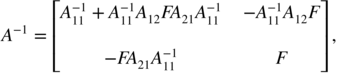
where

-
6.8 (Does the OLS asymptotic variance depend on
ω
0
?)
- Show that for an ARCH(
q
) model
 is proportional to
  (when it exists).
 - Using Exercise 6.7, show that, for an ARCH( q ) model, the asymptotic variance of the OLS estimator of the α 0i does not depend on ω 0 .
- Show that the asymptotic variance of the OLS estimator of
ω
0
is proportional to
 .
.
- Show that for an ARCH(
q
) model
-
6.9 (Properties of the projections on closed convex sets) Let
E
be an Hilbert space, with a scalar product 〈·, ·〉 and a norm ‖ · ‖. When
C ⊂ E
and
x ∈ E
, it is said that
x
* ∈ C
is a best approximation of
x
on
C
if ‖x − x
*‖ = min
y ∈ C
‖x − y‖.
- Show that if C is closed and convex, x * exists and is unique. This point is then called the projection of x on C .
- Show that
x
*
satisfies the so‐called variational inequalities:6.17and prove that x * is the unique point of C satisfying these inequalities.

-
6.10 (Properties of the projections on closed convex cones) Recall that a subset
K
of the vectorial space is a cone if for all
y ∈ K
and for all
λ ≥ 0, we have
λy ∈ K
. Let
K
be a closed convex cone of the Hilbert space
E
.
- Show that the projection
x
*
of
x ∈ E
on
K
(see Exercise 6.9) is characterised by6.18

- Show that
x
*
satisfies
- (a) ∀x ∈ E, ∀ λ ≥ 0, (λx)* = λx *.
- (b) ∀x ∈ E, ‖x‖2 = ‖x *‖2 + ‖x − x *‖2, thus ‖x *‖ ≤ ‖x‖.
- Show that the projection
x
*
of
x ∈ E
on
K
(see Exercise 6.9) is characterised by
-
6.11 (OLS estimation of a subvector of parameters) Consider the linear model
Y = Xθ + U
with the usual assumptions. Let
M
2
be the matrix of the orthogonal projection on the orthogonal subspace of
X
(2)
, where
X = (X
(1), X
(2)). Show that the OLS estimator of
θ
(1)
(where
 , with obvious notation) is
  .
. -
6.12 (A matrix result used in the proof of Theorem 6.7) Let (J
n
) be a sequence of symmetric
k × k
matrices converging to a positive definite matrix
J
. Let (X
n
) be a sequence of vectors in ℝ
k
such that
 . Show that
X
n
→ 0.
. Show that
X
n
→ 0.
- 6.13 (Example of constrained estimator calculus) Take the example of Exercise 6.3 and compute the constrained estimator.