9.1.1 Asymptotic Behaviour

Under the above‐mentioned regularity assumptions, the initial conditions are asymptotically negligible and, using the ergodic theorem, we have almost surely

using Jensen's inequality and the fact that

Adapting the proof of the consistency of the QMLE, it can be shown that almost surely as n → ∞.

Assuming in particular that θ ₀ belongs to the interior of the parameter space, a Taylor expansion yields

9.2

We have

9.3

It is easy to see that (ν _t , ℱ _t ) is a martingale difference (using, for instance, the computations of Exercise 9.1). It follows that

9.4

where ℑ is the Fisher information matrix, defined by

Note that ζ _f is equal to σ ² times the Fisher information for the scale parameter σ > 0 of the densities σ ⁻¹ f(⋅/σ). When f is the (0,1) density, we thus have ζ _f  = σ ² × 2/σ ² = 2.

We now turn to the other terms of the Taylor expansion (9.2). Let

We have

9.5

thus, using the invertibility of ℑ ,

9.6

Note that

9.7

With the previous notation, the QMLE has the asymptotic variance

9.8

The following proposition shows that the QMLE is not only optimal in the Gaussian case.

Note that when f is of the form ( 9.9) then we have

up to a constant which does not depend on θ . It follows that in this case the MLE coincides with the QMLE, which entails the sufficient part of Proposition 9.1.

9.1.2 One‐Step Efficient Estimator

Figure 9.1 shows the graph of the family of densities for which the QMLE and MLE coincide (and thus for which the QML is efficient). When the density f does not belong to this family of distributions, we have ζ _f (∫x ⁴ f(x)dx − 1) > 4, and the QMLE is asymptotically inefficient in the sense that

is positive definite. Table 9.1 shows that the efficiency loss can be important.

An efficient estimator can be obtained from a simple transformation of the QMLE, using the following result (which is intuitively true by (9.7)).

In practice, one can take the QMLE as a preliminary estimator: .

9.1.3 Semiparametric Models and Adaptive Estimators

In general, the density f of the noise is unknown, but f and f ^′ can be estimated from the normalised residuals , t = 1,…, n (for instance, using a kernel non‐parametric estimator). The estimator (or the one‐step estimator ) can then be utilised. This estimator is said to be adaptive if it inherits the efficiency property of for any value of f . In general, it is not possible to estimate all the GARCH parameters adaptively.

Take the ARCH(1) example

9.11

where η _t has the double Weibull density

The subscript 0 is added to signify the true values of the parameters. The parameter , where θ ₀ = (ω ₀, α ₀)^′ , is estimated by maximising the likelihood of the observations ε₁,…, ε _n conditionally on the initial value ε₀ . In view of (9.3), the first two components of the score are given by

with

The last component of the score is

Note that

where γ = 0.577… is the Euler constant. It follows that the score satisfies

where

and . By the general properties of an information matrix (see Exercise 9.4 for a direct verification), we also have

The information matrix ℑ being such that ℑ ₁₂ ≠ 0, the necessary Stein's condition (see Bickel 1982) for the existence of an adaptive estimator is not satisfied. The intuition behind this condition is the following. In view of the previous discussion, the asymptotic variance of the MLE of ϑ ₀ should be of the form

When λ ₀ is unknown, the optimal asymptotic variance of a regular estimator of θ ₀ is thus ℑ ¹¹ . Knowing λ ₀ , the asymptotic variance of the MLE of θ ₀ is . If there exists an adaptive estimator for the class of the densities of the form f _λ (or for a larger class of densities), then we have . Since (see Exercise 6.7), this is possible only if ℑ ₁₂ = 0, which is not the case here.

Reparameterising the model, Drost and Klaassen (1997) showed that it is, however, possible to obtain adaptive estimates of certain parameters. To illustrate this point, return to the ARCH(1) example with the parameterisation

9.12

Let ϑ = (α, c, λ) be an element of the parameter space. The score now satisfies

Thus with

where

It can be seen that this matrix is invertible because its determinant is equal to . Moreover,

The MLE enjoying optimality properties in general, when λ ₀ is unknown, the optimal variance of an estimator of (α ₀, c ₀) should be equal to

When λ ₀ is known, a similar calculation shows that the MLE of (α ₀, c ₀) should have the asymptotic variance

We note that . Thus, in presence of the unknown parameter c , the MLE of α ₀ is equally accurate when λ ₀ is known or unknown. This is not particular to the chosen form of the density of the noise, which leads us to think that there might exist an estimator of α ₀ that adapts to the density f of the noise (in presence of the nuisance parameter c ). Drost and Klaassen (1997) showed the actual existence of adaptive estimators for some parameters of an extension of (9.12).

9.1.4 Local Asymptotic Normality

In this section, we will see that the GARCH model satisfies the so‐called LAN property, which has interesting consequences for the local asymptotic properties of estimators and tests. Let be a sequence of local parameters around the parameter , where (h _n ) is a bounded sequence of ℝ ^{p + q + 1} . Consider the local log‐likelihood ratio function

The Taylor expansion of this function around 0 leads to

9.13

where, as we have already seen,

9.14

It follows that

The properties (9.13)–(9.14) are called LAN. It entails that the MLE is locally asymptotically optimal (in the minimax sense and in various other senses; see van der Vaart 1998). The LAN property also makes it very easy to compute the local asymptotic distributions of statistics, or the asymptotic local powers of tests. As an example, consider tests of the null hypothesis

against the sequence of local alternatives

The performance of the Wald, score, and of likelihood ratio tests will be compared.

Wald Test Based on the MLE

Let be the (q + 1)th component of the MLE . In view of ( 9.7) and ( 9.13)–( 9.14), we have under H ₀ that

9.15

where , and e _i denotes the ith vector of the canonical basis of ℝ ^{p + q + 1} , noting that the (q + 1)th component of is equal to α ₀ . Consequently, the asymptotic distribution of the vector defined in (9.15) is

9.16

Le Cam's third lemma (see van der Vaart 1998, p. 90; see also Exercise 9.3) and the contiguity of the probabilities and (implied by the LAN properties ( 9.13)–( 9.14)) show that, for ,

The Wald test (and also the t test) is defined by the rejection region where

and denotes the (1 − α )‐quantile of a chi‐square distribution with 1 degree of freedom. This test has asymptotic level α and local asymptotic power , where Φ _c (⋅) denotes the cumulative distribution function of a non‐central chi‐square with 1 degree of freedom and non‐centrality parameter ¹

This test is locally asymptotically uniformly most powerful among the asymptotically unbiased tests.

Score Test Based on the MLE

The score (or Lagrange multiplier) test is based on the statistic

9.17

where is the MLE under H ₀ , that is, constrained by the condition that the (q + 1)th component of the estimator is equal to α ₀ . By the definition of , we have

9.18

In view of (9.17) and (9.18), the test statistic can be written as

9.19

Under H ₀ , almost surely and . Consequently,

and

Taking the difference, we obtain

9.20

which, using ( 9.17), gives

9.21

From (9.20), we obtain

Using this relation, and ( 9.18), it follows that

Using (9.19), we have

9.22

By Le Cam's third lemma, the score test thus inherits the local asymptotic optimality properties of the Wald test.

Likelihood Ratio Test Based on the MLE

The likelihood ratio test is based on the statistic . The Taylor expansion of the log‐likelihood around leads to

thus, using , (9.5) and (9.21),

under H ₀ and H _n . It follows that the three tests exhibit the same asymptotic behaviour, both under the null hypothesis and under local alternatives.

Tests Based on the QML

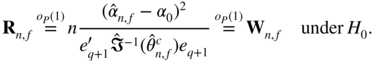
We have seen that the W _{n, f} , R _{n, f} , and L _{n, f} tests based on the MLE are all asymptotically equivalent under H ₀ and H _n (in particular, they are all asymptotically locally optimal). We now compare these tests to those based on the QMLE, focusing on the QML Wald whose statistic is

where is the (q + 1)th component of the QML , and is

or an asymptotically equivalent estimator.

Recall that

Using ( 9.13)–( 9.14), (9.8), and Exercise 9.2, we obtain

under H ₀ . The previous arguments, in particular Le Cam's third lemma, show that

The local asymptotic power of the test is thus , where the non‐centrality parameter is

Figure 9.2 displays the local asymptotic powers of the two tests, (solid line) and (dashed line), when f is the normalised Student t density with 5 degrees of freedom and when θ ₀ is such that . Note that the local asymptotic power of the optimal Wald test is sometimes twice as large as that of score test.

9.2.1 Condition for the Convergence of to θ ₀

Note that under suitable identifiability conditions, σ _t (θ ₀)/σ _t (θ) = 1 if and only if θ = θ ₀ . For the consistency of the estimator (that is, for θ ^* = θ ₀ ), it is thus necessary for the function σ → E _f g(η ₀, σ), where g(x, σ) = log σh(xσ), to have a unique maximum at 1:

9.25

It is sometimes useful to replace condition (9.25) by one of its consequences that is easier to handle. Assume the existence of

If there exists a neighborhood V(1) of 1 such that the dominated convergence theorem shows that ( 9.25) implies the moment condition

9.26

Obviously, condition ( 9.25) is satisfied for the ML, that is, when h = f (see Exercise 9.5), and also for the QML, as the following example shows.

The following example shows that for condition ( 9.25) to be satisfied, it is sometimes necessary to reparameterise the model and to change the identifiability constraint Eη ² = 1.

The previous examples show that a particular choice of h corresponds to a natural identifiability constraint. This constraint applies to a moment of η _t ( when h is , and E ∣ η _t  ∣  = 1 when h is Laplace). Table 9.3 gives the natural identifiability constraints associated with various choices of h . When these natural identifiability constraints are imposed on the GARCH model, the estimator can be interpreted as a non‐Gaussian QMLE, and converges to θ ₀ , even when h ≠ f .

Law	Instrumental density h	Constraint
Gaussian
Double gamma
Laplace		E ∣η t ∣  = 1
Gamma
Double inverse gamma
Double inverse χ 2
Double Weibull		E|η t | λ  = 1
Gaussian generalised		E|η t | λ  = 1
Inverse Weibull		E|η t |−λ  = 1
Double log‐normal		E log  ∣η t ∣  = m

9.2.2 Convergence of and Interpretation of the Limit

The following examples show that the estimator based on the mis‐specified density h ≠ f generally converges to a value θ ^* ≠ θ ₀ which can be interpreted in a reparameterised model.

9.2.3 Choice of Instrumental Density h

We have seen that, for any fixed h , there exists an identifiability constraint implying the convergence of to θ ₀ (see Table  9.3). In practice, we do not choose the parameterisation for which converges, but the estimator that guarantees a consistent estimation of the model of interest. The instrumental function h is chosen to estimate the model under a given constraint, corresponding to a given problem. As an example, suppose that we wish to estimate the conditional moment of a GARCH (p, q) process. It will be convenient to consider the parameterisation ε _t  = σ _t η _t under the constraint . The volatility σ _t will then be directly related to the conditional moment of interest, by the relation . In this particular case, the Gaussian QMLE is inconsistent (because, in particular, the QMLE of α _i converges to ). In view of (9.26), to find relevant instrumental functions h , one can solve

since and E{1 + h ^′(x)/h(η _t )η _t } = 0. The densities that solve this differential equation are of the form

For λ = 1, we obtain the double Weibull, and for λ = 4 a generalised Gaussian, which is in accordance with the results given in Table  9.3.

For the more general problem of estimating conditional moments of ∣ε _t ∣ or log ∣ ε _t ∣, Table 9.4 gives the parameterisation (that is, the moment constraint on η _t ) and the type of estimator (that is, the choice of h ) for the solution to be only a function of the volatility σ _t (a solution which is thus independent of the distribution f of η _t ). It is easy to see that for the instrumental function h of Table  9.4, the estimator depends only on r and not on c and λ . Indeed, taking the case r > 0, up to some constant we have

Problem	Constraint	Solution	Instrumental density, h
E t − 1|ε t | r , r > 0	E|η t | r  = 1		c|x| λ − 1 exp(−λ|x| r /r), λ > 0
E t − 1|ε t |−r	E|η t |−r  = 1		c|x|−λ − 1 exp(−λ|x|−r /r)
E t − 1 log |ε t |	E log |η t | = 0	log σ t

which shows that does not depend on c and λ . In practice, one can thus choose the simplest constants in the instrumental function, for instance c = λ = 1.

9.2.4 Asymptotic Distribution of

Using arguments similar to those of Section 7.4, a Taylor expansion shows that, under ( 9.25),

where

and

The ergodic theorem and the CLT for martingale increments (see Section A.2) then entail that

9.27

where

9.28

with g ₁(x, σ) = ∂g(x, σ)/∂σ and g ₂(x, σ) = ∂g ₁(x, σ)/∂σ .

Table 9.5 completes Table  9.1. Using the previous examples, this table gives the ARE of the QMLE and Laplace QMLE with respect to the MLE, in the case where f follows the Student t distribution. The table does not allow us to obtain the ARE of the QMLE with respect to Laplace QMLE, because the noise η _t has a different normalisation with the standard QMLE or the Laplace QMLE (in other words, the two estimators do not converge to the same parameter).

	ν
	5	6	7	8	9	10	20	30	100
MLE – QMLE	2.5	1.667	1.4	1.273	1.2	1.154	1.033	1.014	1.001
MLE – Laplace	1.063	1.037	1.029	1.028	1.030	1.034	1.070	1.089	1.124

For the QMLE, the Student t density f _ν with ν degrees of freedom is normalised so that Eη_t ² = 1, that is, the density of η _t is . For the Laplace QMLE, η _t has the density f(y) = E ∣ t _ν  ∣ f _ν (yE ∣ t _ν ∣), so that E ∣ η _t  ∣  = 1.

9.3.1 Weighted LSE for the ARMA Parameters

Consider the estimation of the ARMA part of the ARMA(P, Q)‐GARCH (p, q) model

9.29

where (η _t ) is an iid(0,1) sequence and the coefficients ω ₀ , α _0i and β _0j satisfy the usual positivity constraints. The orders P, Q, p , and q are assumed known. The parameter vector is

the true value of which is denoted by ϑ ₀ , and the parameter space Ψ ⊂ ℝ ^{P + Q + 1} . Given observations X ₁,…, X _n and initial values, the sequence is defined recursively by (7.22). The weighted LSE is defined as a measurable solution of

where the weights ω _t are known positive measurable functions of X _t − 1, X _t − 2, …. One can take, for instance,

with E|X ₁|^2s  < ∞ and s ∈ (0, 1). It can be shown that there exist constants K > 0 and ρ ∈ (0, 1) such that

This entails that

Thus

which implies a finite variance for the score vector . Ling (2005) deduces the asymptotic normality of , even in the case

9.3.2 Self‐Weighted QMLE

Recall that, for the ARMA‐GARCH models, the asymptotic normality of the QMLE has been established under the condition (see Theorem 7.5). To obtain an asymptotically normal estimator of the parameter of the ARMA‐GARCH model (9.29) with weaker moment assumptions on the observed process, Ling (2007) proposed a self‐weighted QMLE of the form

where , using standard notation. To understand the principle of this estimator, note that the minimised criterion converges to the limit criterion l(ϕ) = E _ϕ ω _t ℓ _t (ϕ) satisfying

The last expectation (when it exists) is null, because η _t is centred and independent of the other variables. The inequality x − 1 ≥ log x entails that

Thus, under the usual identifiability conditions, we have l(ϕ) ≥ l(ϕ ₀), with equality if and only if ϕ = ϕ ₀ . Note that the orthogonality between η _t and the weights ω _t is essential. Ling (2007) showed the convergence and asymptotic normality of under the assumption E|X ₁| ^s  < ∞ for some s > 0.

9.3.3 L _p Estimators

The previous weighted estimator requires the assumption . Practitioners often claim that financial series admit few moments. A GARCH process with infinite variance is obtained either by taking large values of the parameters, or by taking an infinite variance for η _t . Indeed, for a GARCH(1, 1) process, each of the two sets of assumptions

1. (i) ,
2. (ii)

implies an infinite variance for ε _t . Under (i), and strict stationarity, the asymptotic distribution of the QMLE is generally Gaussian (see Section 7.1.1), whereas the usual estimators have non‐standard asymptotic distributions under (ii) (see Berkes and Horváth 2003b; Hall and Yao 2003; Mikosch and Straumann 2002), which causes difficulties for inference. As an alternative to the QMLE, it is thus interesting to define estimators having an asymptotic normal distribution under (ii), or even in the more general situation where both α ₀₁ + β ₀₁ > 1 and are allowed. A GARCH model is usually defined under the normalisation constraint . When the assumption that exists is relaxed, the GARCH coefficients can be identified by imposing, for instance, that the median of is τ = 1. In the framework of ARCH(q) models, Horváth and Liese (2004) consider L _p estimators, including the L ₁ estimator

where, for instance, . When admits a density, continuous and positive around its median τ = 1, the consistency and asymptotic normality of these estimators are shown in Horváth and Liese (2004), without any moment assumption. An alternative to L _p ‐estimators, which only requires and can be applied to ARMA‐GARCH, is the self‐weighted quasi‐maximum exponential likelihood estimator studied by Zhu and Ling (2011).

9.3.4 Least Absolute Value Estimation

For ARCH and GARCH models, Peng and Yao (2003) studied several least absolute deviations estimators. An interesting specification is

9.30

With this estimator, it is convenient to define the GARCH parameters under the constraint that the median of is 1. A reparameterisation of the standard GARCH models is thus necessary. Consider, for instance, a GARCH(1, 1) with parameters ω , α ₁ and β ₁ , and a Gaussian noise η _t . Since the median of is τ = 0.4549…, the median of the square of is 1, and the model is rewritten as

It is interesting to note that the error terms are iid with median 0 when θ = θ ₀ . Intuitively, this is the reason why it is pointless to introduce weights in the sum (9.30). Under the moment assumption and some regularity assumptions, Peng and Yao (2003) show that there exists a local solution of ( 9.30) which is weakly consistent and asymptotically normal, with rate of convergence n ^1/2 . This convergence holds even when the distribution of the errors has a fat tail: only the moment condition is required.

9.3.5 Whittle Estimator

In Chapter 2, we have seen that, under the condition that the fourth‐order moments exist, the square of a GARCH(p, q) satisfies the ARMA(max(p, q), q) representation

9.31

where

The spectral density of is

Let be the empirical autocovariance of at lag h . At Fourier frequencies λ _j  = 2πj/n ∈ (−π, π], the periodogram

can be considered as a non‐parametric estimator of . Let

It can be shown that

with equality if and only if θ = θ ₀ (see Proposition 10.8.1 in Brockwell and Davis 1991). In view of this inequality, it is natural to consider the so‐called Whittle estimator

For ARMA with iid innovations, the Whittle estimator has the same asymptotic behaviour as the QMLE and LSE (which coincide in that case). For GARCH models, the Whittle estimator still exhibits the same asymptotic behaviour as the LSE, but it is generally less accurate than the QMLE. Moreover, Giraitis and Robinson (2001), Mikosch and Straumann (2002), and Straumann (2005) have shown that the consistency requires the existence of , and that the asymptotic normality requires .

9.5 Exercises

9.1 (The score of a scale parameter is centred)

Show that if f is a differentiable density such that ∫ ∣ x ∣ f(x)dx < ∞, then

Deduce that the score vector defined by ( 9.3) is centred.

1. 9.2 (Covariance between the square and the score of the scale parameter) Show that if f is a differentiable density such that ∫|x|³ f(x)dx < ∞, then
   
2. 9.3 (Intuition behind Le Cam's third lemma) Let φ _θ (x) = (2πσ ²)^−1/2 exp(−(x − θ)²/2σ ²) be the density and let the log‐likelihood ratio
   

   Determine the distribution of

   

   when , and then when .

3. 9.4 (Fisher information) For the parametrisation (9.11), verify that
   
4. 9.5 (Condition for the consistency of the MLE) Let η be a random variable with density f such that E|η| ^r  < ∞ for some r ≠ 0. Show that
   
5. 9.6 (Case where the Laplace QMLE is optimal) Consider a GARCH model whose noise has the Γ(b, b) distribution with density
   

   where b > 0. Show that the Laplace QMLE is optimal.

6. 9.7 (Comparison of the MLE, QMLE and Laplace QMLE) Give a table similar to Table  9.5, but replace the Student t distribution f _ν by the double Γ(b, p) distribution
   

   where b, p > 0.

7. 9.8 (Asymptotic comparison of the estimators ) Compute the coefficient defined by (9.28) for each of the instrumental densities h of Table  9.4. Compare the asymptotic behaviour of the estimators .

8. 9.9 (Fisher information at a pseudo‐true value)

   Consider a GARCH (p, q) model with parameter
   
   1. Give an example of an estimator which does not converge to θ ₀ , but which converges to a vector of the form
      
      where ϱ is a constant.
   2. What is the relationship between and ?
   3. Let Λ_ϱ = diag(ϱ⁻² I _q + 1, I _p ) and
      

      Give an expression for J(θ ^*) as a function of J(θ ₀) and Λ_ϱ .

9. 9.10 (Asymptotic distribution of the Laplace QMLE) Determine the asymptotic distribution of the Laplace QMLE when the GARCH model does not satisfy the natural identifiability constraint E ∣ η _t  ∣  = 1, but the usual constraint .