10
Multivariate GARCH Processes
While the volatility of univariate series has been the focus of the previous chapters, modelling the co‐movements of several series is of great practical importance. When several series displaying temporal or contemporaneous dependencies are available, it is useful to analyse them jointly, by viewing them as the components of a vector‐valued (multivariate) process. The standard linear modelling of real‐time series has a natural multivariate extension through the framework of the vector ARMA (VARMA) models. In particular, the subclass of vector autoregressive (VAR) models has been widely studied in the econometric literature. This extension entails numerous specific problems and has given rise to new research areas (such as co‐integration).
Similarly, it is important to introduce the concept of multivariate GARCH (MGARCH) model. For instance, asset pricing and risk management crucially depend on the conditional covariance structure of the assets of a portfolio. Unlike the ARMA models, however, the GARCH model specification does not suggest a natural extension to the multivariate framework. Indeed, the (conditional) expectation of a vector of size m is a vector of size m, but the (conditional) variance is an m × m matrix. A general extension of the univariate GARCH processes would involve specifying each of the m(m + 1)/2 entries of this matrix as a function of its past values and the past values of the other entries. Given the excessive number of parameters that this approach would entail, it is not feasible from a statistical point of view. An alternative approach is to introduce some specification constraints which, while preserving a certain generality, make these models operational.
We start by reviewing the main concepts for the analysis of the multivariate time series.
10.1 Multivariate Stationary Processes
In this section, we consider a vector process (X t ) t ∈ ℤ of dimension m, X t = (X 1t ,…,X mt )′. The definition of strict stationarity (see Chapter 1, Definition 1.1) remains valid for vector processes, while second‐order stationarity is defined as follows.
Obviously, Γ X (h) = Γ X (−h)′ . In particular, Γ X (0) = Var(X t ) is a symmetric matrix.
The simplest example of a multivariate stationary process is white noise, defined as a sequence of centred and uncorrelated variables whose covariance matrix is time‐independent.
The following property can be used to construct a stationary process by linear transformation of another stationary process.
The proof of an analogous result is given by Brockwell and Davis (1991, pp. 83–84) and the arguments used extend straightforwardly to the multivariate setting. When, in this theorem, (Z t ) is a white noise and C k = 0 for all k < 0, (X t ) is called a vector moving average process of infinite order, VMA(∞). A multivariate extension of Wold's representation theorem (see Hannan 1970, pp. 157–158) states that if (X t ) is a stationary and purely non‐deterministic process, it can be represented as an infinite‐order moving average,

where (ε
t
) is a (m × 1) white noise,
B
is the lag operator, ![]() , and the matrices
C
k
are not necessarily absolutely summable but satisfy the (weaker) condition
, and the matrices
C
k
are not necessarily absolutely summable but satisfy the (weaker) condition ![]() , for any matrix norm ‖ · ‖. The following definition generalises the notion of a scalar ARMA process to the multivariate case.
, for any matrix norm ‖ · ‖. The following definition generalises the notion of a scalar ARMA process to the multivariate case.
Denote by det(A), or more simply ∣A∣ when there is no ambiguity, the determinant of a square matrix A . A sufficient condition for the existence of a stationary and invertible solution to the preceding equation is
(see Brockwell and Davis 1991, Theorems 11.3.1 and 11.3.2).
When p = 0, the process is called vector moving average of order q (VMA(q)); when q = 0, the process is called VAR of order p (VAR(p)).
Note that the determinant ∣Φ(z)∣ is a polynomial admitting a finite number of roots z 1,…, z mp . Let δ = min i ∣ z i ∣ > 1. The power series expansion

where A * denotes the adjoint of the matrix A (that is, the transpose of the matrix of the cofactors of A ), is well defined for ∣z ∣ < δ , and is such that Φ(z)−1Φ(z) = I . The matrices C k are recursively obtained by

10.2 Multivariate GARCH Models
As in the univariate case, we can define MGARCH models by specifying their first two conditional moments. An ℝ m ‐valued GARCH process (ε t ), with ε t = (ε1t ,…, ε mt )′ , must then satisfy, for all t ∈ ℤ,
The multivariate extension of the notion of the strong GARCH process is based on an equation of the form
where (η
t
) is a sequence of iid ℝ
m
‐valued variables with zero mean and identity covariance matrix. The square root has to be understood in the sense of the Cholesky factorization, that is, ![]() . The matrix
. The matrix ![]() can be chosen to be symmetric and positive definite,
1
but it can also be chosen to be triangular, with positive diagonal elements (see, for instance, Harville 1997, Theorem 14.5.11). The latter choice may be of interest because if, for instance,
can be chosen to be symmetric and positive definite,
1
but it can also be chosen to be triangular, with positive diagonal elements (see, for instance, Harville 1997, Theorem 14.5.11). The latter choice may be of interest because if, for instance, ![]() is chosen to be lower triangular, the first component of ε
t
only depends on the first component of
η
t
. When
m = 2, we can thus set
is chosen to be lower triangular, the first component of ε
t
only depends on the first component of
η
t
. When
m = 2, we can thus set

where η it and h ij, t denote the generic elements of η t and H t .
Note that any square integral solution (ε t ) of (10.6) is a martingale difference satisfying (10.5).
Choosing a specification for H t is obviously more delicate than in the univariate framework because (i) H t should be (almost surely) symmetric, and positive definite for all t ; (ii) the specification should be simple enough to be amenable to probabilistic study (existence of solutions, stationarity, etc.), while being of sufficient generality; (iii) the specification should be parsimonious enough to enable feasible estimation. However, the model should not be too simple to be able to capture the – possibly sophisticated – dynamics in the covariance structure.
Moreover, it may be useful to have the so‐called stability by aggregation property. If ε
t
satisfies ( 10.5), the process ![]() defined by
defined by ![]() , where
P
is an invertible square matrix, is such that
, where
P
is an invertible square matrix, is such that
The stability by aggregation of a class of specifications for
H
t
requires that the conditional variance matrices ![]() belong to the same class for any choice of
P
. This property is particularly relevant in finance because if the components of the vector ε
t
are asset returns,
belong to the same class for any choice of
P
. This property is particularly relevant in finance because if the components of the vector ε
t
are asset returns, ![]() is a vector of portfolios of the same assets, each of its components consisting of amounts (coefficients of the corresponding row of
P
) of the initial assets.
is a vector of portfolios of the same assets, each of its components consisting of amounts (coefficients of the corresponding row of
P
) of the initial assets.
10.2.1 Diagonal Model
A popular specification, known as the diagonal representation, is obtained by assuming that each element h kℓ, t of the covariance matrix H t is formulated in terms only of the product of the prior k and ℓ returns. Specifically,

with
ω
kℓ = ω
ℓk
, ![]() ,
, ![]() for all (k, ℓ). For
m = 1, this model coincides with the usual univariate formulation. When
m > 1, the model obviously has a large number of parameters and will not in general produce positive definite covariance matrices
H
t
. We have
for all (k, ℓ). For
m = 1, this model coincides with the usual univariate formulation. When
m > 1, the model obviously has a large number of parameters and will not in general produce positive definite covariance matrices
H
t
. We have

where ⊙ denotes the Hadamard product, that is, the element by element product. 2 Thus, in the ARCH case ( p = 0), sufficient positivity conditions are that Ω is positive definite and the A (i) are positive semi‐definite, but these constraints do not easily generalise to the GARCH case. We shall give further positivity conditions obtained by expressing the model in a different way, viewing it as a particular case of a more general class.
It is easy to see that the model is not stable by aggregation: for instance, the conditional variance of ε1, t
+ ε2, t
can in general be expressed as a function of the ![]() and
and ![]() , but not of the (ε1, t − i
+ ε2, t − i
)2
. A final drawback of this model is that there is no interaction between the different components of the conditional covariance, which appears unrealistic for applications to financial series.
, but not of the (ε1, t − i
+ ε2, t − i
)2
. A final drawback of this model is that there is no interaction between the different components of the conditional covariance, which appears unrealistic for applications to financial series.
In what follows, we present the main specifications introduced in the literature, before turning to the existence of solutions. Let η denote a probability distribution on ℝ m , with zero mean and unit covariance matrix.
10.2.2 Vector GARCH Model
The vector GARCH (VEC‐GARCH) model is the most direct generalisation of univariate GARCH: every conditional covariance is a function of lagged conditional variances as well as lagged cross‐products of all components. In some sense, everything is explained by everything, which makes this model not only very general but also not very parsimonious.
Denote by vech(·) the operator that stacks the columns of the lower triangular part of its argument square matrix (if A = (a ij ), then vech(A) = (a 11, a 21,…, a m1, a 22,…, a m2,…, a mm )′ ). The next definition is a natural extension of the standard GARCH( p, q ) specification.
Positivity Conditions
To ensure the positive semi-definiteness of Ht , the initial values and Ω (where ω = vech(Ω)) have to be positive semi‐definite, and the matrices A(i) and B(j) need to map the vectorized positive semi‐definite matrices into themselves. To be more specific, a generic element of
is denoted by
h
kℓ, t
(
k ≥ ℓ), and we will denote by ![]() (
(![]() ) the entry of
A
(i)
(
B
(j)
) located on the same row as
h
kℓ, t
and belonging to the same column as the element
) the entry of
A
(i)
(
B
(j)
) located on the same row as
h
kℓ, t
and belonging to the same column as the element ![]() of
of ![]() . We thus have an expression of the form
. We thus have an expression of the form

Denoting by ![]() the
m × m
symmetric matrix with (k
′, ℓ′)th entry
the
m × m
symmetric matrix with (k
′, ℓ′)th entry ![]() , for
k
′ ≠ ℓ′
, and the elements
, for
k
′ ≠ ℓ′
, and the elements ![]() on the diagonal, the preceding equality is written as
on the diagonal, the preceding equality is written as

In order to obtain a more compact form for the last part of this expression, let us introduce the spectral decomposition of the symmetric matrices
H
t
, assumed to be positive semi‐definite. We have ![]() , where
, where ![]() is an orthogonal matrix of eigenvectors
is an orthogonal matrix of eigenvectors ![]() associated with the (positive) eigenvalues
associated with the (positive) eigenvalues ![]() of
H
t
. Defining the matrices
of
H
t
. Defining the matrices ![]() by analogy with the
by analogy with the ![]() , we get
, we get

Finally, consider the
m
2 × m
2
matrix admitting the block form ![]() , and let
, and let ![]() . The preceding expressions are equivalent to
. The preceding expressions are equivalent to

where Ω is the symmetric matrix such that vech(Ω) = ω .
In this form, it is evident that the assumption
ensures that if the H t − j are almost surely positive definite, then so is H t .
10.2.3 Constant Conditional Correlations Models
Suppose that, for a MGARCH process of the form ( 10.6), all the past information on ε
kt
, involving all the variables εℓ, t − i
, is summarised in the variable
h
kk, t
, with ![]() . Then, letting
. Then, letting ![]() , we define for all
k
a sequence of iid variables with zero mean and unit variance. The variables
, we define for all
k
a sequence of iid variables with zero mean and unit variance. The variables ![]() are generally correlated, so let
are generally correlated, so let ![]() , where
, where ![]() . The conditional variance of
. The conditional variance of
is then written as
By construction, the conditional correlations between the components of ε t are time‐invariant:

To complete the specification, the dynamics of the conditional variances h kk, t has to be defined. The simplest constant conditional correlations (CCC) model relies on the following univariate GARCH specifications:

where ω k > 0, a k, i ≥ 0, b k, j ≥ 0, −1 ≤ ρ kℓ ≤ 1, ρ kk = 1, and R is symmetric and positive semi‐definite. Observe that the conditional variances are specified as in the diagonal model. The conditional covariances clearly are not linear in the squares and cross products of the returns.
In a multivariate framework, it seems natural to extend the specification (10.17) by allowing h kk, t to depend not only on its own past, but also on the past of all the variables εℓ, t . Set

We have ![]() where
where ![]() is a centred vector with covariance matrix
R
. The components of ε
t
thus have the usual expression,
is a centred vector with covariance matrix
R
. The components of ε
t
thus have the usual expression, ![]() , but the conditional variance
h
kk, t
depends on the past of all the components of ε
t
.
, but the conditional variance
h
kk, t
depends on the past of all the components of ε
t
.
Note that the conditional covariances are generally non‐linear functions of the components of ![]() and of past values of the components of
H
t
. Model (10.18) is thus not a VEC‐GARCH model, defined by ( 10.9), except when
R
is the identity matrix.
and of past values of the components of
H
t
. Model (10.18) is thus not a VEC‐GARCH model, defined by ( 10.9), except when
R
is the identity matrix.
One advantage of this specification is that a simple condition ensuring the positive definiteness of H t is obtained through the positive coefficients for the matrices A i and B j and the choice of a positive definite matrix for R . Conrad and Karanasos (2010) showed that less restrictive assumptions ensuring the positive definiteness of Ht can be found. Moreover there exists a representation of the CCC model in which the matrices Bj are diagonal. Another advantage of the CCC specification is that the study of the stationarity is remarkably simple.
Two limitations of the CCC model are, however, (i) its non‐stability by aggregation and (ii) the arbitrary nature of the assumption of constant conditional correlations.
10.2.4 Dynamic Conditional Correlations Models
Dynamic conditional correlations GARCH (DCC‐GARCH) models are an extension of CCC‐GARCH, obtained by introducing a dynamic for the conditional correlation. Hence, the constant matrix R in Definition 10.4 is replaced by a matrix R t which is measurable with respect to the past variables {ε u , u < t}. For reasons of parsimony, it seems reasonable to choose diagonal matrices A i and B i in ( 10.18), corresponding to univariate GARCH models for each component as in ( 10.17). Different DCC models are obtained depending on the specification of R t . A simple formulation is
where the θ i are positive weights summing to 1, R is a constant correlation matrix, and Ψ t − 1 is the empirical correlation matrix of ε t − 1,…, ε t − M . The matrix R t is thus a correlation matrix (see Exercise 10.9). Equation (10.19) is reminiscent of the GARCH(1, 1) specification, θ 1 R playing the role of the parameter ω , θ 2 that of α , and θ 3 that of β .
Another way of specifying the dynamics of R t is by setting
where diag Q
t
is the diagonal matrix constructed with the diagonal elements of
Q
t
, and
Q
t
is a sequence of covariance matrices which is measurable with respect to
σ(ε
u
, u < t). In the original DCC model of Engle (2002), the dynamics of ![]() is given by
is given by
where ![]() denotes the vector of standardized returns,
denotes the vector of standardized returns, ![]() , and
, and ![]() is a positive‐definite matrix.
is a positive‐definite matrix.
Matrix ![]() turns out to be difficult to interpret, and Aielli (2013) pointed out that
turns out to be difficult to interpret, and Aielli (2013) pointed out that ![]() in general. Thus, the commonly used estimator of
in general. Thus, the commonly used estimator of ![]() defined as the sample second moment of the standardized returns is not consistent in this formulation.
defined as the sample second moment of the standardized returns is not consistent in this formulation.
In the so‐called corrected DCC (cDCC) model of Aielli (2013), the dynamics of ![]() is reformulated as
is reformulated as
under the same constraints on the coefficients. In this model, under stationarity conditions, ![]() .
.
Multiplying the left‐hand side and the right‐hand side of ![]() by an arbitrary positive‐definite matrix yields the same conditional correlation matrix
by an arbitrary positive‐definite matrix yields the same conditional correlation matrix ![]() . It is thus necessary to introduce an identifiability condition, as for instance imposing that
. It is thus necessary to introduce an identifiability condition, as for instance imposing that ![]() be a correlation matrix.
be a correlation matrix.
10.2.5 BEKK‐GARCH Model
The BEKK acronym refers to a specific parameterisation of the MGARCH model developed by Baba, Engle, Kraft, and Kroner, in a preliminary version of Engle and Kroner (1995).
The specification obviously ensures that if the matrices, H t − i , i = 1,…, p , are almost surely positive definite, then so is H t .
To compare this model with the representation ( 10.9), let us derive the vector form of the equation for H t . Using the relations (10.10) and (10.11), we get

The model can thus be written in the VEC‐GARCH(p,q) form ( 10.9), with

for i = 1,…, q and j = 1,…, p . In particular, it can be seen that the number of coefficients of a matrix A (i) in ( 10.9) is [m(m + 1)/2]2 , whereas it is Km 2 in this particular case. However, the converse is not true. Stelzer (2008) showed that, for m ≥ 3, there exist VEC-GARCH models that cannot be represented in the BEKK form.
The BEKK class contains (Exercise 10.13) the diagonal models obtained by choosing diagonal matrices A ik and B jk . The following theorem establishes a converse to this property.
It is interesting to consider the stability by aggregation of the BEKK class.
As in the univariate case, the ‘square’ of the (ε
t
) process is the solution of an ARMA model. Indeed, define the innovation of the process ![]() :
:
Applying the vec operator, and substituting the variables vec(H
t − j
) in the model of Definition 10.5 by ![]() , we get the representation
, we get the representation

where r = max(p, q), with the convention A ik = 0 ( B jk = 0) if i > q ( j > p ). This representation cannot be used to obtain stationarity conditions because the process (ν t ) is not iid in general. However, it can be used to derive the second‐order moment, when it exists, of the process ε t as

that is,

provided that the matrix in braces is non‐singular.
10.2.6 Factor GARCH Models
In these models, it is assumed that a non‐singular linear combination f t of the m components of ε t , or an exogenous variable summarising the co‐movements of the components, has a GARCH structure.
Factor Models with Idiosyncratic Noise
A very popular factor model links individual returns ε it to the market return f t through a regression model
The parameter β i can be interpreted as a sensitivity to the factor, and the noise η it as a specific risk (often called idiosyncratic risk) which is conditionally uncorrelated with f t . It follows that H t = Ω + λ t β β ′ , where β = (β1,…, β m )′ is the vector of sensitivities, λ t is the conditional variance of f t , and Ω is the covariance matrix of the idiosyncratic terms. More generally, assuming the existence of r conditionally uncorrelated factors, we obtain the decomposition

It is not restrictive to assume that the factors are linear combinations of the components of ε t (Exercise 10.10). If, in addition, the conditional variances λ jt are specified as univariate GARCH, the model remains parsimonious in terms of unknown parameters and (10.25) reduces to a particular BEKK model (Exercise 10.11). If Ω is chosen to be positive definite and if the univariate series (λ jt ) t , j = 1,…, r are independent, strictly and second‐order stationary, then it is clear that ( 10.25) defines a sequence of positive definite matrices (H t ) that are strictly and second‐order stationary.
Principal Components GARCH Model
The concept of factor is central to principal components analysis (PCA) and to other methods of exploratory data analysis. PCA relies on decomposing the covariance matrix V of m quantitative variables as V = PΛP ′ , where Λ is a diagonal matrix whose elements are the eigenvalues λ 1 ≥ λ 2 ≥ ⋯ ≥ λ m of V , and where P is the orthonormal matrix of the corresponding eigenvectors. The first principal component is the linear combination of the m variables, with weights given by the first column of P, which, in some sense, is the factor which best summarises the set of m variables (Exercise 10.12). There exist m principal components, which are uncorrelated and whose variances λ 1,…, λ m (and hence whose explanatory powers) are in decreasing order. It is natural to consider this method for extracting the key factors of the volatilities of the m components of ε t .
We obtain a principal component GARCH (PC‐GARCH) or orthogonal GARCH (O‐GARCH) model by assuming that
where P is an orthogonal matrix ( P ′ = P −1 ) and Λ t = diag(λ 1t ,…, λ mt ), where the λ it are the volatilities, which can be obtained from univariate GARCH‐type models. This is equivalent to assuming
where
f
t
= P
′ε
t
is the principal component vector, whose components are orthogonal factors. If univariate GARCH(1, 1) models are used for the factors ![]() , then
, then
10.2.7 Cholesky GARCH
Suppose that the conditional covariance matrix H t of ε t is positive‐definite, i.e. that the components of ε t are not multicolinear. Given the information ℱ t − 1 generated by the past values of ε t , let ℓ21, t be the conditional beta in the regression of ε2t on v 1t ≔ ε1t . One can write
with β 21, t = ℓ21, t ∈ ℱ t − 1 , and υ 2t is orthogonal to ε1t conditionally on ℱ t − 1 . More generally, we have

where υ it is uncorrelated with υ 1t ,…, υ i − 1, t , and thus uncorrelated with ε1t ,…, ε i − 1, t , conditionally on ℱ t − 1 . In matrix form, Eq. (10.31) is written as
where
L
t
and ![]() are lower unitriangular (i.e. triangular with 1 on the diagonal) matrices, with ℓ
ij, t
(respectively −β
ij, t
) at row
i
and column
j
of
L
t
(respectively
B
t
) for
i > j
. For
m = 3, we have
are lower unitriangular (i.e. triangular with 1 on the diagonal) matrices, with ℓ
ij, t
(respectively −β
ij, t
) at row
i
and column
j
of
L
t
(respectively
B
t
) for
i > j
. For
m = 3, we have

The vector υ t of the error terms in the linear regressions ( 10.31) can be interpreted as a vector of orthogonal factors, whose covariance matrix is G t = diag(g 1t ,…, g mt ) with g it > 0 for i = 1,…, m . We then obtain the so‐called Cholesky decomposition of the covariance matrix of ε t :
Note that the Cholesky decomposition also extends to positive semi‐definite matrices.
Taking ![]() , we obtain
, we obtain ![]() . A simple parametric form of the volatility
. A simple parametric form of the volatility ![]() of the
i
th factor
υ
it
could be of the GARCH(1,1)‐type
of the
i
th factor
υ
it
could be of the GARCH(1,1)‐type
In view of the results of the Chapter 2, a necessary and sufficient condition for the existence of a strictly stationary process (υ t ) in this parameterisation is
Of course, Eq. (10.33) could also include explanatory variables ![]() with
j ≠ i
, or other variables belonging
with
j ≠ i
, or other variables belonging ![]() .
.
To obtain a complete parametric specification for H t , it now suffices to specify a time series model for the conditional betas, i.e. for the elements of L t (or alternatively for those of B t ). Note that this model can be quite general because, to ensure the positive‐definiteness of H t , the conditional betas are not a priori subject to any constraint.
For instance, one can assume a dynamics of the form
where f ij is a real‐valued function, depending on υ t − 1 and on some parameter θ , and c ij is a real coefficient. Under the conditions ∣c ij ∣ < 1, and the condition (10.34) ensuring the existence of the stationary sequence (υ t ), there exists a stationary solution to Eq. (10.35). The Cholesky decomposition (10.32) then provides a model for the conditional covariance matrix H t .
The absence of strong constraints on the coefficients constitutes an attractive feature of the Cholesky decomposition ( 10.32), compared in particular to the DCC decomposition ![]() for which the unexplicit constraints of positive definiteness of
R
t
render the determination of stationarity conditions challenging. Another obvious interest of the Cholesky approach is to provide a direct way to predict the conditional betas, which appear to be of primary interest for particular financial applications (see Engle 2016).
for which the unexplicit constraints of positive definiteness of
R
t
render the determination of stationarity conditions challenging. Another obvious interest of the Cholesky approach is to provide a direct way to predict the conditional betas, which appear to be of primary interest for particular financial applications (see Engle 2016).
Now, let us briefly explore the relationships between the Cholesky decomposition and the factor models. Suppose that the first k < m columns of the matrix L t are constant so that L t = [P : P t ] with P a non‐random matrix of size m × k and P t of size m × (m − r). The Cholesky GARCH can then be interpreted as a factor model:
where
f
t
= (υ
1t
,…, υ
kt
)′
is a vector of
k
orthogonal factors,
P
is called the loading matrix and u
t
= P
t
(υ
k + 1, t
,…, υ
mt
)′
is a so‐called idiosyncratic disturbance (independent of
f
t
). If ε
t
is a vector of excess returns (i.e. each component is the return of a risky asset minus the return of a risk free asset), and if the first component is the excess return of the market portfolio, in the one‐factor case (
k = 1) the previous factor model corresponds to the Capital Asset Pricing Model (CAPM) of Sharpe (1964), Lintner (1965), and Merton (1973). More precisely, we have
P = (1, β
′)′
, where
β
represents the ‘sensitivity of returns to market returns’, and ![]() . Denoting by
r
t
= (ε2t
,…, ε
mt
)′
the vector of excess returns, the last (m − 1) lines of the one‐factor model gives the CAPM equation
. Denoting by
r
t
= (ε2t
,…, ε
mt
)′
the vector of excess returns, the last (m − 1) lines of the one‐factor model gives the CAPM equation
where υ 1t is the market excess return.
10.3 Stationarity
In this section, we will first discuss the difficulty of establishing stationarity conditions, or the existence of moments, for MGARCH models. For the general vector model ( 10.9), and in particular for the BEKK model, there exist sufficient stationarity conditions. The stationary solution being non‐explicit, we propose an algorithm that converges, under certain assumptions, to the stationary solution. We will then see that the problem is much simpler for the CCC model ( 10.18).
10.3.1 Stationarity of VEC and BEKK Models
It is not possible to provide stationary solutions, in explicit form, for the general VEC model ( 10.9). To illustrate the difficulty, recall that a univariate ARCH(1) model admits a solution ε t = σ t η t with σ t explicitly given as a function of {η t − u , u > 0} as the square root of
provided that the series converges almost surely. Now consider a bivariate model of the form ( 10.6) with ![]() where
α
is assumed, for the sake of simplicity, to be scalar and positive. Also choose
where
α
is assumed, for the sake of simplicity, to be scalar and positive. Also choose ![]() to be a lower triangular so as to have Eq. (10.7). Then
to be a lower triangular so as to have Eq. (10.7). Then

It can be seen that given η t − 1 , the relationship between h 11, t and h 11, t − 1 is linear, and can be iterated to yield

under the constraint ![]() . In contrast, the relationships between
h
12, t
, or
h
22, t
, and the components of
H
t − 1
are not linear, which makes it impossible to express
h
12, t
and
h
22, t
as a simple function of
α
, {η
t − 1, η
t − 2,…, η
t − k
} and
H
t − k
for
k ≥ 1. This constitutes a major obstacle for determining sufficient stationarity conditions.
. In contrast, the relationships between
h
12, t
, or
h
22, t
, and the components of
H
t − 1
are not linear, which makes it impossible to express
h
12, t
and
h
22, t
as a simple function of
α
, {η
t − 1, η
t − 2,…, η
t − k
} and
H
t − k
for
k ≥ 1. This constitutes a major obstacle for determining sufficient stationarity conditions.
In the particular case of the BEKK model of Definition 10.5, condition (iii) takes the form
The proof of Theorem 10.5 relies on sophisticated algebraic tools. Assumption (ii) is a standard technical condition for showing the
β
‐mixing property (but is of no use for stationarity). Note that condition (iii), written as ![]() in the univariate case, is generally not necessary for the strict stationarity.
in the univariate case, is generally not necessary for the strict stationarity.
This theorem does not provide explicit stationary solutions, that is, a relationship between ε t and the η t − i . However, it is possible to construct an algorithm which, when it converges, allows a stationary solution to the vector GARCH model ( 10.9) to be defined.
Construction of a Stationary Solution
For any t, k ∈ ℤ, we define
and, recursively on k ≥ 0,

with ![]() .
.
Observe that, for k ≥ 1,
where
f
k
is a measurable function and
H
(k)
is a square matrix. The processes ![]() and
and ![]() are thus stationary with components in the Banach space
L
2
of the (equivalence classes of) square integral random variables. It is then clear that Eq. ( 10.9) admits a strictly stationary solution, which is non‐anticipative and ergodic, if, for all
t
,
are thus stationary with components in the Banach space
L
2
of the (equivalence classes of) square integral random variables. It is then clear that Eq. ( 10.9) admits a strictly stationary solution, which is non‐anticipative and ergodic, if, for all
t
,
Indeed, letting ![]() and
and ![]() , and taking the limit of each side of (10.36), we note that ( 10.9) is satisfied. Moreover, (ε
t
) constitutes a strictly stationary and non‐anticipative solution, because ε
t
is a measurable function of {η
u
, u ≤ t}. In view of Theorem A.1, such a process is also ergodic. Note also that if
H
t
exists, it is symmetric and positive definite because the matrices
, and taking the limit of each side of (10.36), we note that ( 10.9) is satisfied. Moreover, (ε
t
) constitutes a strictly stationary and non‐anticipative solution, because ε
t
is a measurable function of {η
u
, u ≤ t}. In view of Theorem A.1, such a process is also ergodic. Note also that if
H
t
exists, it is symmetric and positive definite because the matrices ![]() are symmetric and satisfy
are symmetric and satisfy
This solution (ε t ) is also second‐order stationary if
Let
From Exercise 10.8 and its proof, we obtain (10.37), and hence the existence of strictly stationary solution to the vector GARCH ( 10.9), if there exists
ρ ∈ (0, 1) such that ![]() almost surely as
k → ∞, which is equivalent to
almost surely as
k → ∞, which is equivalent to
Similarly, we obtain (10.38) if ![]() . The criterion in (10.39) is not very explicit but the left‐hand side of the inequality can be evaluated by simulation, just as for a Lyapunov coefficient.
. The criterion in (10.39) is not very explicit but the left‐hand side of the inequality can be evaluated by simulation, just as for a Lyapunov coefficient.
10.3.2 Stationarity of the CCC Model
In model ( 10.18), letting ![]() , we get
, we get

Multiplying by ϒ
t
the equation for ![]() , we thus have
, we thus have

which can be written
where

and

is a (p + q)m × (p + q)m matrix.
We obtain a vector representation, analogous to (2.16) obtained in the univariate case. This allows us to state the following result.
The following result provides a necessary strict stationarity condition which is simple to check.
10.3.3 Stationarity of DCC models
Stationarity conditions for the DCC model, with the specification (10.19) for R t , have been established by Fermanian and Malongo (2016). However, except in very specific cases, such conditions are non explicit. The corrected DCC model allows for more tractable conditions. Sufficient stationarity conditions – based on the results by Boussama, Fuchs and Stelzer (2011) – are provided for the cDDD model by Aielli (2013).
10.4 QML Estimation of General MGARCH
In this section, we define the quasi‐maximum likelihood estimator (QMLE) of a general MGARCH model, and we provide high‐level assumptions entailing its strong consistency and asymptotic normality (CAN). In the next section, these assumptions will be made more explicit for the particular case of the CCC‐GARCH model.
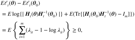
Assume a general parametric conditional variance H t = H t (θ 0), with an unknown d ‐dimensional parameter θ 0 . Let Θ be a compact parameter space which contains θ 0 . For all θ = (θ 1,…, θ d )′ ∈ Θ, assume that
For particular MGARCH models, it is possible to write
H
t
as a measurable function of {η
u
, u < t}, which entails that (ε
t
) is stationary and ergodic (see the ergodic theorem, Theorem A.1). In (10.46), the matrix
H
t
(θ) is written as a function of the past observations. A model satisfying this requirement is said to be invertible at
θ
. For prediction purposes, it is obviously necessary that a model of parameter
θ
0
be invertible at
θ
0
. For estimating
θ
0
, it seems also crucial that the model possesses this property at any
θ ∈ Θ, since the estimation methods are typically based on comparisons between ![]() and
H
t
(θ), for all observations ε
t
and all values of
θ ∈ Θ.
and
H
t
(θ), for all observations ε
t
and all values of
θ ∈ Θ.
Given observations ε1,…, ε
n
, and arbitrary fixed initial values ![]() for
i ≤ 0, let the statistics
for
i ≤ 0, let the statistics
A QMLE of
θ
0
is defined as any measurable solution ![]() of
of

Note that the QMLE would be simply the maximum likelihood estimation if the conditional distribution of ε t was Gaussian with mean zero and variance H t .
10.4.1 Asymptotic Properties of the QMLE
Let ![]() ,
,

Recall that ρ denotes a generic constant belonging to [0, 1), and K denotes a positive constant or a positive random variable measurable with respect to {ε u , u < 0} (and thus which does not depend on n ). The regularity conditions (which do not depend on the choice of the norms) are the following.
- A1:
 a.s.
a.s. - A2:
 a.s.
a.s. - A3: E‖ε t s ‖ < ∞ and E‖H t (θ 0)‖ s < ∞ for some s > 0.
- A4: For θ ∈ Θ, H t (θ) = H t (θ 0) a.s. implies θ = θ 0 .
- A5: For any sequence x 1, x 2,… of vectors of ℝ m , the function θ ↦ H(x 1, x 2,…; θ) is continuous on Θ.
- A6:
θ
0
belongs to the interior
 of Θ.
of Θ. - A7: For any sequence x 1, x 2,… of vectors of ℝ m , the function θ ↦ H(x 1, x 2,…; θ) admits continuous second‐order derivatives.
- A8: For some neighbourhood
V(θ
0) of
θ
0
,

- A9: For some neighbourhood
V(θ
0) of
θ
0
, for all
i, j ∈ {1,…, m} and
p > 1,
q > 2 and
r > 2 such that 2q
−1 + 2r
−1 = 1 and
p
−1 + 2r
−1 = 1, we have
5

- A10: E ∥ η t ∥4 < ∞.
- A11: The matrices {∂ H t (θ 0)/∂θ i , i = 1,…, d} are linearly independent with non‐zero probability.
In the case
m = 1, Assumption A1 requires that the volatility be bounded away from zero uniformly on Θ. For a standard GARCH satisfying
ω > 0 and Θ compact, the assumption is satisfied. Assumption A2 is related to the invertibility and entails that
H
t
(θ) is well estimated by the statistic ![]() when
t
is large. For some models it will be useful to replace A2 by the weaker, but more complicated, assumption
when
t
is large. For some models it will be useful to replace A2 by the weaker, but more complicated, assumption
- A2':
 where
ρ
t
is a random variable satisfying
where
ρ
t
is a random variable satisfying  , for some
p > 1 and
s ∈ (0, 1) satisfying A3.
, for some
p > 1 and
s ∈ (0, 1) satisfying A3.
This assumption, as well as A8, will be used to show that the choice of the initial values ![]() is asymptotically unimportant. Corollary 10.2 shows that, for some particular models, the strict stationarity implies the existence of marginal moments, as required in A3. Assumption A4 is an identifiability condition. As shown in Section 8.2, A6 is necessary to obtain the asymptotic normality (AN) of the QMLE. Assumptions A9 and A10 are used to show the existence of the information matrices
I
and
J
involved in the sandwich form
J
−1
IJ
−1
of the asymptotic variance of the QMLE. Assumption A11 is used to show the invertibility of
J
.
is asymptotically unimportant. Corollary 10.2 shows that, for some particular models, the strict stationarity implies the existence of marginal moments, as required in A3. Assumption A4 is an identifiability condition. As shown in Section 8.2, A6 is necessary to obtain the asymptotic normality (AN) of the QMLE. Assumptions A9 and A10 are used to show the existence of the information matrices
I
and
J
involved in the sandwich form
J
−1
IJ
−1
of the asymptotic variance of the QMLE. Assumption A11 is used to show the invertibility of
J
.
10.5 Estimation of the CCC Model
We now turn to the estimation of the m ‐dimensional CCC‐GARCH(p, q) model by the quasi‐maximum likelihood method. Recall that (ε t ) is called a CCC‐GARCH(p, q) if it satisfies

where
R
is a correlation matrix, ![]() is a vector of size
m × 1 with strictly positive coefficients, the
A
i
and
B
j
are matrices of size
m × m
with positive coefficients, and (η
t
) is a sequence of iid centred variables in ℝ
m
with identity covariance matrix.
is a vector of size
m × 1 with strictly positive coefficients, the
A
i
and
B
j
are matrices of size
m × m
with positive coefficients, and (η
t
) is a sequence of iid centred variables in ℝ
m
with identity covariance matrix.
As in the univariate case, the criterion is written as if the iid process were Gaussian.
The parameters are the coefficients of the matrices ![]() ,
A
i
and
B
j
, and the coefficients of the lower triangular part (excluding the diagonal) of the correlation matrix
R = (ρ
ij
). The number of unknown parameters is thus
,
A
i
and
B
j
, and the coefficients of the lower triangular part (excluding the diagonal) of the correlation matrix
R = (ρ
ij
). The number of unknown parameters is thus
The parameter vector is denoted by
where ρ ′ = (ρ 21,…, ρ m1, ρ 32,…, ρ m2,…, ρ m, m − 1), α i = vec(A i ), i = 1,…, q, and β j = vec(B j ), j = 1,…, p . The parameter space is a subspace Θ of
The true parameter value is denoted by
Before detailing the estimation procedure and its properties, we discuss the conditions that need to be imposed on the matrices A i and B j in order to ensure the uniqueness of the parameterisation.
10.5.1 Identifiability Conditions
Let ![]() By convention,
By convention, ![]() if
q = 0 and ℬ
θ
(z) = I
m
if
p = 0.
if
q = 0 and ℬ
θ
(z) = I
m
if
p = 0.
If ℬ
θ
(z) is non‐singular, that is, if the roots of det(ℬ
θ
(z)) = 0 are outside the unit disk, we deduce from ![]() the representation
the representation
In the vector case, assuming that the polynomials ![]() and
and ![]() have no common root is insufficient to ensure that there exists no other pair
have no common root is insufficient to ensure that there exists no other pair ![]() , with the same degrees (p, q), such that
, with the same degrees (p, q), such that
This condition is equivalent to the existence of an operator U(B) such that
this common factor vanishing in ℬ θ (B)−1 풜 θ (B) (Exercise 10.2).
The polynomial U(B) is called unimodular if det{U(B)} is a non‐zero constant. When the only common factors of the polynomials P(B) and Q(B) are unimodular, that is, when
then P(B) and Q(B) are called left coprime.
The following example shows that, in the vector case, assuming that ![]() and
and ![]() are left coprime is insufficient to ensure that condition (10.52) has no solution
θ ≠ θ
0
(in the univariate case this is sufficient because the condition
are left coprime is insufficient to ensure that condition (10.52) has no solution
θ ≠ θ
0
(in the univariate case this is sufficient because the condition ![]() imposes
U(B) = U(0) = 1).
imposes
U(B) = U(0) = 1).
10.5.2 Asymptotic Properties of the QMLE of the CCC‐GARCH model
For particular classes of MGARCH models, the assumptions of the previous section can be made more explicit. Let us consider the CCC‐GARCH model. Let (ε1,…, ε
n
) be an observation of length
n
of the unique non‐anticipative and strictly stationary solution (ε
t
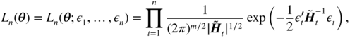
) of model (10.50). Conditionally on non‐negative initial values ![]() , the Gaussian quasi‐likelihood is written as
, the Gaussian quasi‐likelihood is written as
where the ![]() are recursively defined, for
t ≥ 1, by
are recursively defined, for
t ≥ 1, by

A QMLE of θ is defined as in ( 10.47) by:
To establish the AN we require the following additional assumptions:
- CC6:
 , where
  is the interior of
Θ
.
is the interior of
Θ
. - CC7:
10.6 Looking for Numerically Feasible Estimation Methods
Despite the wide range of applicability of the QML estimation method, this approach may entail formidable numerical difficulties when the dimension of the vector of financial returns under study is large. In asset pricing applications or portfolio management, practitioners may have to handle cross sections of hundreds – even thousands – of stocks. Whatever the class of MGARCH used, the number of unknown parameters increases dramatically as the dimension of the cross section increases. This is particularly problematic when the Gaussian QML estimation method is used, because the high‐dimensional conditional variance matrix has to be inverted at every step of the optimisation procedure.
In this section, we present two methods aiming at alleviating the dimensionality curse.
10.6.1 Variance Targeting Estimation
Variance targeting (VT) estimation is a two‐step procedure in which the unconditional variance–covariance matrix of the returns vector process is estimated by a moment estimator in a first step. VT is based on a reparameterisation of the MGARCH model, in which the matrix of intercepts in the volatility equation is replaced by the unconditional covariance matrix.
To be more specific, consider the CCC‐GARCH( p, q ) model

where ![]() and
R
0
is a correlation matrix,
A
0i
and
B
0j
are
m × m
matrices with positive coefficients. Model (10.58) admits a strict and second‐order non‐anticipative stationary solution (ε
t
) when
and
R
0
is a correlation matrix,
A
0i
and
B
0j
are
m × m
matrices with positive coefficients. Model (10.58) admits a strict and second‐order non‐anticipative stationary solution (ε
t
) when
A: the spectral radius of ![]() is strictly less than 1.
is strictly less than 1.
Moreover, under this assumption, we have that

It follows that the last equation in model ( 10.58) can be equivalently written

With this new formulation, the generic parameter value consists of the coefficients of the vector h and the matrices A i and B j (corresponding to the true values h 0, A 0i and B 0j , respectively), and the coefficients of the lower triangular part (excluding the diagonal) of the correlation matrix R = (ρ ij ). One advantage of this parameterisation over the initial one is that the parameter h 0 can be straightforwardly estimated by the empirical mean
In the VT estimation method, the components of h are thus estimated empirically in a first step, and the other parameters are estimated in a second step, via a QML optimisation. Under appropriate assumptions, the resulting estimator is shown to be consistent and asymptotically normal (see Francq, Horváth, and Zakoian 2016).
One interest of this procedure is computational. Table 10.1 shows the reduction of computational time compared to the full quasi‐maximum likelihood (FQML), when both the dimension m of the series and the sample size n vary. For both methods, the computation time increases rapidly with m , but the relative time‐computation gain does not depend much on m , nor on n .
Table 10.1 Seconds of CPU time for computing the VTE and QMLE (average of 100 replications).
Source: Francq, Horváth, and Zakoian (2016).
| n = 500 | n = 5000 | |||||
| m = 2 | m = 3 | m = 4 | m = 2 | m = 3 | m = 4 | |
| VTE | 3.44 | 7.98 | 17.29 | 41.40 | 94.43 | 197.53 |
| QMLE | 5.48 | 13.82 | 25.17 | 65.22 | 145.41 | 284.85 |
One issue is whether the time‐computation gain is paid in terms of accuracy of the estimator. In the univariate case, m = 1 (that is, for a standard GARCH( p, q ) model), it can be shown that the VTE is never asymptotically more efficient than the QMLE, regardless of the values of the GARCH parameters and the distribution of the iid process (see Francq, Horváth, and Zakoian 2011). In the multivariate setting, the asymptotic distributions of the two estimators are difficult to compare but, on simulation experiments, the accuracy loss entailed by the two‐step VT procedure is often barely visible. In finite sample, the VT estimator may even perform much better than the QML estimator.
A nice feature of the VT estimator is that it ensures robust estimation of the marginal variance, provided that it exists. Indeed, the variance of a model estimated by VT converges to the theoretical variance, even if the model is mis‐specified. For the convergence to hold true, it suffices that the observed process be stationary and ergodic with a finite second‐order moment. This is generally not the case when the misspecified model is estimated by QML. For some specific purposes such as long‐horizon prediction or long‐term value‐at‐risk evaluation, the essential point is to well estimate the marginal distribution, in particular the marginal moments. The fact that the VTE guarantees a consistent estimation of the marginal variance may then be a crucial advantage over the QMLE.
10.6.2 Equation‐by‐Equation Estimation
Another approach for alleviating the dimensionality curse in the estimation of MGARCH models consists in estimating the individual volatilities in a first step – ‘equation‐by‐equation’ (EbE) – and to estimate the remaining parameters in a second step.
More precisely, any ℝ m ‐valued process (ε t ) with zero‐conditional mean and positive‐definite conditional variance matrix H t can be represented as

where ![]() is the
σ
‐field generated by {ε
u
, u < t},
D
t
= {diag(
H
t
)}1/2
and
is the
σ
‐field generated by {ε
u
, u < t},
D
t
= {diag(
H
t
)}1/2
and ![]() Let
Let ![]() the
k
th diagonal element of
H
t
, that is the variance of
ε
kt
conditional on
the
k
th diagonal element of
H
t
, that is the variance of
ε
kt
conditional on ![]() . Assuming that
. Assuming that ![]() is parameterised by some parameter
is parameterised by some parameter ![]() , belonging to a compact parameter space
Θ
k
, we can write
, belonging to a compact parameter space
Θ
k
, we can write

where
σ
k
is a positive function. The vector ![]() satisfies
satisfies ![]() and
and ![]() Because
Because ![]() and
and ![]() ,
, ![]() can be called the vector of EbE innovations of (ε
t
).
can be called the vector of EbE innovations of (ε
t
).
It is important to note that model (10.62), satisfied by the components of (ε
t
), is not a standard univariate GARCH. First, because the volatility
σ
kt
depends on the past of all components of ε
t
– not only the past of
ε
kt
. And second, because the innovation sequence ![]() is not iid (except when the conditional correlation matrix is constant,
R
t
=
R
). For instance, a parametric specification of
σ
kt
mimicking the classical GARCH(1,1) is given by
is not iid (except when the conditional correlation matrix is constant,
R
t
=
R
). For instance, a parametric specification of
σ
kt
mimicking the classical GARCH(1,1) is given by

Of course, other formulations – for instance including leverage effects – could be considered as well.
Having parameterised the individual conditional variances of (ε t ), the model can be completed by specifying the dynamics of the conditional correlation matrix R t . For instance, in the DCC model of Engle (2002a), the conditional correlation matrix is modelled as a function of the past standardized returns, as follows
where
α, β ≥ 0, α + β < 1,
S
is a positive‐definite matrix, and ![]() is the diagonal matrix with the same diagonal elements as
Q
t
.
is the diagonal matrix with the same diagonal elements as
Q
t
.
More generally, suppose that matrix R t is parameterised by some parameter ρ 0 ∈ ℝ r , together with the volatility parameter θ 0 , as
Given observations ε1,…, ε
n
, and arbitrary initial values ![]() for
i ≤ 0, we define
for
i ≤ 0, we define ![]() for
k = 1,…, m
. A two‐step estimation procedure can be developed as follows.
for
k = 1,…, m
. A two‐step estimation procedure can be developed as follows.
-
First step: EbE estimation of the volatility parameters
 , by
, by
and extraction of the vectors of residuals
 where
where  ;
; -
Second step: QML estimation of the conditional correlation matrix
ρ
0
, as a solution of10.64

where Λ ⊂ ℝ r is a compact set,
 , and the
  's are initial values.
Asymptotic properties of the procedure can be established for particular models (BEKK, CCC, etc.).
Numerical experiments confirm that the gains in computation time can be huge compared with the FQML estimator in which all the parameters are estimated in one step. Table 10.2 compares the effective computation times required by the two estimators as a function of the dimension
m
, for the CCC‐GARCH(1, 1) model with
A
1 = 0.05
I
m
,
B
1 = 0.9
I
m
,
R
=
I
m
, and ![]() . The
m(m − 1)/2 sub‐diagonal terms of
R
were estimated, together with the 3m
other parameters of the model. The two estimators were fitted on simulations of length
n = 2000. The comparison of the CPUs is clearly in favour of the EbEE, the FQML being in failure for
m ≥ 10. When
m
increases, the computation time of the FQML estimator becomes prohibitive, and more importantly, the optimisation fails to provide a reasonable value for
. The
m(m − 1)/2 sub‐diagonal terms of
R
were estimated, together with the 3m
other parameters of the model. The two estimators were fitted on simulations of length
n = 2000. The comparison of the CPUs is clearly in favour of the EbEE, the FQML being in failure for
m ≥ 10. When
m
increases, the computation time of the FQML estimator becomes prohibitive, and more importantly, the optimisation fails to provide a reasonable value for ![]() . Table 10.2 also compares the relative efficiencies (RE) of the two approaches. To this aim, we first computed the approximated information matrix
. Table 10.2 also compares the relative efficiencies (RE) of the two approaches. To this aim, we first computed the approximated information matrix ![]() . The quadratic form
. The quadratic form ![]() is used as a measure of accuracy of an estimator
is used as a measure of accuracy of an estimator ![]() (the Euclidean distance, obtained by replacing
J
n
by the identity matrix, has the drawback of being scale dependent). The relative efficiency displayed in Table 10.2 is defined by
(the Euclidean distance, obtained by replacing
J
n
by the identity matrix, has the drawback of being scale dependent). The relative efficiency displayed in Table 10.2 is defined by

Table 10.2 Computation time (CPU time in seconds) and relative efficiency (RE) of the EbE with respect to the FQMLE (NA = not available, due to the impossibility to compute the FQMLE), for m ‐dimensional CCC‐GARCH(1,1) models.
Source: Francq and Zakoïan (2016).
| Dim. m | 2 | 4 | 6 | 8 | 10 |
| No. of parameters | 7 | 18 | 33 | 52 | 75 |
| CPU for EbEE | 0.57 | 1.18 | 1.52 | 2.04 | 2.82 |
| CPU for FQMLE | 32.49 | 123.33 | 317.85 | 876.52 | 1 292.34 |
| ratio of CPU | 57.00 | 104.52 | 209.11 | 429.67 | 458.28 |
| RE | 0.96 | 0.99 | 0.99 | 0.97 | 102.42 |
| Dim. m | 50 | 100 | 200 | 400 | 800 |
| No. of parameters | 1 375 | 5 250 | 20 500 | 81 000 | 322 000 |
| CPU for EbEE | 13.67 | 27.89 | 56.58 | 110.00 | 226.32 |
| CPU for FQMLE | NA | NA | NA | NA | NA |
| Ratio of CPU | NA | NA | NA | NA | NA |
| RE | NA | NA | NA | NA | NA |
where ![]() and
and ![]() denote, respectively, the EbE and FQML estimators. The computation time of the FQML estimator being huge when
m
is large, the RE and CPU times are only computed on 1 simulation, but they are representative of what is generally observed. When
m ≤ 9, the accuracies are very similar, with a slight advantage for the FQML (which corresponds here to the ML). When the number of parameters becomes too large, the optimisation fails to give a reasonable value of
denote, respectively, the EbE and FQML estimators. The computation time of the FQML estimator being huge when
m
is large, the RE and CPU times are only computed on 1 simulation, but they are representative of what is generally observed. When
m ≤ 9, the accuracies are very similar, with a slight advantage for the FQML (which corresponds here to the ML). When the number of parameters becomes too large, the optimisation fails to give a reasonable value of ![]() , and the RE clearly indicates the superiority of the EbEE over the QMLE for
m ≥ 10.
, and the RE clearly indicates the superiority of the EbEE over the QMLE for
m ≥ 10.
10.7 Proofs of the Asymptotic Results
10.7.1 Proof of the CAN in Theorem 10.7
We shall use the multiplicative norm (see Exercises 10.5 and 10.6) defined by
where
A
is a
d
1 × d
2
matrix, ∥x∥ is the Euclidean norm of vector ![]() , and
ρ(·) denotes the spectral radius. This norm satisfies, for any
d
2 × d
1
matrix
B
,
, and
ρ(·) denotes the spectral radius. This norm satisfies, for any
d
2 × d
1
matrix
B
,

When A is a square d × d matrix, the last inequality of (10.68) yields
We also often use the elementary relation
when A is a d 1 × d 2 matrix and B is d 2 × d 1 matrix.
To show the AN, we will use the following elementary results on the differentiation of expressions involving matrices. If f(A) is a real‐valued function of a matrix A whose entries a ij are functions of some variable x , the chain rule for differentiation of compositions of functions states that

Moreover, for A invertible we have
Proof of the Consistency
We shall establish the intermediate results (a), (c), and (d) which are stated as in the univariate case (see the proof of Theorem 7.1 in Section 7.4), the result (b) being satisfied by Assumption A4.
Proof of (a): initial values are forgotten asymptotically. We have

Using (10.71), (10.69), A1–A2, and omitting the subscript ‘( θ )’, the first sum of (10.79) satisfies

as
n → ∞. Indeed ![]() is finite a.s. since, for some
s < 1,
is finite a.s. since, for some
s < 1,

by A3. If A2 is replaced by A2′, the previous result follows from the Hölder inequality. Now, consider the second term of the right‐hand side of ( 10.79). The relation (10.70), the Minkowski inequality, the elementary inequality log(x) ≤ x + 1 and the multiplicativity of the spectral matrix norm imply

and, by symmetry,
Using again A1, A2, or A2′, we thus have shown that
Proof of (c): the limit criterion is minimised at the true value. As in the univariate case, we first show that
Eℓ
t
(
θ
) is well defined in ℝ ∪ {+∞} for all
θ
, and in ℝ for
θ
=
θ
0
. By A1 and ( 10.70) we have ![]() and thus
and thus
At θ 0 , Jensen's inequality and A3 entail
Now we show that
Eℓ
t
(
θ
) is minimised at
θ
0
. Without loss of generality, assume that ![]() . Let
λ
1, t
,…, λ
m, t
be the eigenvalues of
. Let
λ
1, t
,…, λ
m, t
be the eigenvalues of ![]() , which are positive (see Exercise 10.15). We have
, which are positive (see Exercise 10.15). We have
where the inequality is strict unless if λ it = 1 a.s. for all i , that is iff H t ( θ ) = H t ( θ 0) a.s., which is equivalent to θ = θ 0 under A4.
Proof of (d). The previous results and the ergodic theorem then entail that
Similarly, (10.80) and the ergodic theorem applied to the stationary process (X
t
) with ![]() show that
show that

where
V
m
(
θ
) denotes the ball of centre
θ
and radius 1/m
. By A1 we have ![]() . Subtracting the constant
K
0
to ℓ
t
(
θ
*) if necessary, one can always assume that
. Subtracting the constant
K
0
to ℓ
t
(
θ
*) if necessary, one can always assume that ![]() is positive. If
E ∣ ℓ
t
(
θ
) ∣ < ∞, by Fatou's lemma and A5, for any
ε > 0 there exists
m
sufficiently large such that
is positive. If
E ∣ ℓ
t
(
θ
) ∣ < ∞, by Fatou's lemma and A5, for any
ε > 0 there exists
m
sufficiently large such that
If ![]() , then the left‐hand side of the previous inequality can be made arbitrarily large. The consistency follows.
, then the left‐hand side of the previous inequality can be made arbitrarily large. The consistency follows.
Proof of the Asymptotic Normality (AN)
The matrix derivative rules (10.72), (10.77), and (10.75) yield
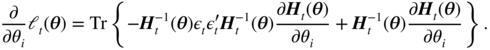
We thus have
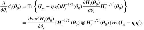
Under A10, the matrix
K
is well defined, and the second moment condition in A9 entails
E ∥
C
i, t
∥2 < ∞. The existence of the matrix
I
is thus guaranteed by A9 and A10. It is then clear from (10.82) that ![]() is a square integrable stationary and ergodic martingale difference. The central limit theorem in Corollary A.1 and the Cramér–Wold device then entail that
is a square integrable stationary and ergodic martingale difference. The central limit theorem in Corollary A.1 and the Cramér–Wold device then entail that

Differentiating (10.81), we also have
with

Under A9, noting that Ec 1( θ 0) = − Ec 4( θ 0) and Ec 3( θ 0) = − Ec 5( θ 0), we thus have

using elementary properties of the vec and Kronecker operators. By the consistency and A6, we have ![]() , and thus almost surely
, and thus almost surely ![]() for
n
large enough. Taylor expansions and A7–A8 thus show that almost surely
for
n
large enough. Taylor expansions and A7–A8 thus show that almost surely

where the ![]() 's are between
's are between ![]() and
θ
0
component‐wise. To show that the previous matrix into brackets converges almost surely to
J
, it suffices to use the ergodic theorem, the continuity of the derivatives, and to show that
and
θ
0
component‐wise. To show that the previous matrix into brackets converges almost surely to
J
, it suffices to use the ergodic theorem, the continuity of the derivatives, and to show that

for some neighbourhood V( θ 0) of θ 0 , which follows from A7 and A9.
If
J
was singular, there would exist some non‐zero vector
λ
∈ ℝ
d
such that
λ
′
Jλ
= 0. Since ![]() is almost surely positive definite, this entails that
Δ
t
λ
= 0 with probability one, which is excluded by A10. The AN, as well as the Bahadur linearisation (10.49), easily follow from (10.83).
is almost surely positive definite, this entails that
Δ
t
λ
= 0 with probability one, which is excluded by A10. The AN, as well as the Bahadur linearisation (10.49), easily follow from (10.83).
10.7.2 Proof of the CAN in Theorems 10.8 and 10.9
The proof consists in showing that the regularity conditions of Theorem 10.7 are satisfied.
Proof of Theorem 10.8
Note that CC2 implies that the invertibility condition ( 10.46) holds for all θ ∈ Θ , and that H t = H t ( θ 0) is a measurable function of { η u , u < t}. Corollary 10.2 shows that, under the stationarity condition CC2, the moment conditions A3 are satisfied. The smoothness conditions A5 and A7 are obviously satisfied for the CCC model.
Proof that A1 and A2′ are satisfied: Rewrite Eq. (10.57) in matrix form as
where ![]() is defined in Corollary 10.1 and
is defined in Corollary 10.1 and

In view of assumption CC2 and Corollary 10.1, we have ![]() By the compactness of
Θ
, we even have
By the compactness of
Θ
, we even have
Corollary 10.2 and (10.86) thus entail that
for some s > 0. Using Eq. (10.84) iteratively, as in the univariate case, we deduce that almost surely
where ![]() denotes the vector obtained by replacing the variables
denotes the vector obtained by replacing the variables ![]() by
by ![]() in
H
t
. Observe that
K
is a random variable that depends on the past values {ε
t
, t ≤ 0}. Since
K
does not depend on
n
, it can be considered as a constant, like
ρ
. We deduce that
in
H
t
. Observe that
K
is a random variable that depends on the past values {ε
t
, t ≤ 0}. Since
K
does not depend on
n
, it can be considered as a constant, like
ρ
. We deduce that
where the second inequality is obtained by arguing that the elements of ![]() are strictly positive uniformly in
Θ
. We then have
are strictly positive uniformly in
Θ
. We then have
with ρ t = ρ t sup θ ∈ Θ ∥ D t ∥. Therefore, the second moment condition of (10.87) shows that A2′ holds true, for any p and for s sufficiently small.
Noting that ∥
R
−1∥ is the inverse of the eigenvalue of smallest modulus of
R
, and that ![]() , we have
, we have
using CC5, the compactness of
Θ
and the strict positivity of the components of ![]() . Similarly, we have
. Similarly, we have
We thus have shown that A1 and A2′ hold true, meaning that the initial values are asymptotically irrelevant, in the sense of ( 10.80).
Proof of A4: Suppose that, for some θ ≠ θ 0 ,
Then it readily follows that ρ = ρ 0 and, using the invertibility of the polynomial ℬ θ (B) under assumption CC2, by ( 10.87),
that is,

Let ![]() . Noting that
. Noting that ![]() and isolating the terms that are functions of
η
t − 1
,
and isolating the terms that are functions of
η
t − 1
,
where
Z
t − 2
belongs to the
σ
‐field generated by {η
t − 2, η
t − 3,…}. Since
η
t − 1
is independent of this
σ
‐field, Exercise 10.3 shows that the latter equality contradicts CC3 unless when
p
ij
h
jj, t
= 0 almost surely, where the
p
ij
are the entries of ![]() for
i, j = 1,…, m
. Because
h
jj, t
> 0 for all
j
, we thus have
for
i, j = 1,…, m
. Because
h
jj, t
> 0 for all
j
, we thus have ![]() . Similarly, we show that
. Similarly, we show that ![]() by successively considering the past values of
η
t − 1
. Therefore, in view of CC4 (or CC4
′
), we have
α = α
0
and
β = β
0
by arguments already used. It readily follows that
by successively considering the past values of
η
t − 1
. Therefore, in view of CC4 (or CC4
′
), we have
α = α
0
and
β = β
0
by arguments already used. It readily follows that ![]() . Hence
θ
=
θ
0
. We have thus established the identifiability condition A4, and the proof of Theorem 10.8 follows from Theorem 10.7.□
. Hence
θ
=
θ
0
. We have thus established the identifiability condition A4, and the proof of Theorem 10.8 follows from Theorem 10.7.□
Proof of Theorem 10.9
It remains to show that A8, A9 and A11 hold.
Proof of A9: Denoting by ![]() the
i
1
th component of
the
i
1
th component of ![]() ,
,

where
c
0
is a strictly positive constant and, by the usual convention, the index 0 corresponds to quantities evaluated at
θ
=
θ
0
. Under CC6, for a sufficiently small neighbourhood ![]() of
θ
0
, we have
of
θ
0
, we have

for all
i
1, j
1, j
2 ∈ {1,…, m} and all
δ > 0. Moreover, in ![]() , the coefficient of
, the coefficient of ![]() is bounded below by a constant
c > 0 uniformly on
is bounded below by a constant
c > 0 uniformly on ![]() . We thus have
. We thus have

for some
ρ ∈ [0, 1), all
δ > 0 and all
s ∈ [0, 1]. Corollary 10.2 then implies that, for all
r
0 ≥ 0, there exists ![]() such that
such that

Since
where R 0 denotes the true value of R , the last moment condition of A9 is satisfied (for all r ).

and, setting s 2 = m + qm 2 ,
Setting s 1 = m + (p + q)m 2 , we have

where ![]() is a matrix whose entries are all 0, apart from a 1 located at the same place as
θ
i
in
is a matrix whose entries are all 0, apart from a 1 located at the same place as
θ
i
in ![]() . By abuse of notation, we denote by
H
t
(i
1) and
. By abuse of notation, we denote by
H
t
(i
1) and ![]() the
i
1
th components of
H
t
and
the
i
1
th components of
H
t
and ![]() . Note that, by the arguments used to show ( 10.87), the previous expressions show that
. Note that, by the arguments used to show ( 10.87), the previous expressions show that

for some s > 0. With arguments similar to those used in the univariate case, that is, the inequality x/(1 + x) ≤ x s for all x ≥ 0 and s ∈ [0, 1], and the inequalities

and, setting ![]() ,
,

we obtain

where the constants ![]() (which also depend on
i
1
,
s
and
r
0
) belong to the interval [0, 1). Noting that these inequalities are uniform on a neighbourhood of
(which also depend on
i
1
,
s
and
r
0
) belong to the interval [0, 1). Noting that these inequalities are uniform on a neighbourhood of ![]() , that they can be extended to higher‐order derivatives, and that Corollary 10.2 implies that
, that they can be extended to higher‐order derivatives, and that Corollary 10.2 implies that ![]() , we can show, as in the univariate case, that for all
i
1 = 1,…, m
, all
i, j, k = 1,…, s
1
and all
r
0 ≥ 0, there exists a neighbourhood
, we can show, as in the univariate case, that for all
i
1 = 1,…, m
, all
i, j, k = 1,…, s
1
and all
r
0 ≥ 0, there exists a neighbourhood ![]() of
θ
0
such that
of
θ
0
such that

and

Omitting ‘( θ )’ to lighten the notation, note that

for i = 1,…, s 1 , and
for i = s 1 + 1,…, s 0 . It follows that (10.93) entails the second moment condition of A9 (for any q ). Similarly, (10.94) entails the first moment condition of A9 (for any p ).
Proof of A8: First note that by
From Eq. ( 10.84), we have

where
r = max {p, q} and the tilde means that initial values are taken into account. Since ![]() for all
t > r
, we have
for all
t > r
, we have ![]() and
and

Thus condition ( 10.86) entails that

Because
the second inequality of ( 10.88) and (10.96) imply that

Note that ( 10.81) continues to hold when ℓ
t
(
θ
) and
H
t
(
θ
) are replaced by ![]() and
and ![]() . Therefore,
. Therefore,

where

Using conditions ( 10.87), (10.90), ( 10.91), (10.92), (10.95), and (10.97), it can be shown that Tr(
C
1 +
C
2) ≤ Kρ
t
u
t
, where u
t
is a random variable such that sup
t
E|u
t
|
s
< ∞ for some small
s ∈ (0, 1). Arguing that ![]() is almost surely finite because its moment of order
s
is finite, the conclusion follows.
is almost surely finite because its moment of order
s
is finite, the conclusion follows.
Proof of A11: Recall that we applied Theorem 10.7 with
d = s
0
. We thus have to show that it cannot exist as a non‐zero vector ![]() , such that
, such that ![]() with probability 1. Decompose
c
into
with probability 1. Decompose
c
into ![]() with
with ![]() and
and ![]() , where
s
3 = s
0 − s
1 = m(m − 1)/2. Rows 1, m + 1,…, m
2
of the equations
, where
s
3 = s
0 − s
1 = m(m − 1)/2. Rows 1, m + 1,…, m
2
of the equations

give

Differentiating Eq. ( 10.57) yields

where
Because (10.99) is satisfied for all t , we have

where quantities evaluated at θ = θ 0 are indexed by 0. This entails that

and finally, introducing a vector θ 1 whose s 1 first components are
we have
by choosing c 1 small enough so that θ 1 ∈ Θ . If c 1 ≠ 0 then θ 1 ≠ θ 0 . This is in contradiction to the identifiability of the parameter (see the proof of A4), hence c 1 = 0. Equations (10.98) thus become

Therefore,
Because the vectors, ∂vec
R
/∂θ
i
,
i = s
1 + 1,…, s
0
, are linearly independent, the vector ![]() is null, and thus
c = 0, which completes the proof.□
is null, and thus
c = 0, which completes the proof.□
10.8 Bibliographical Notes
Multivariate ARCH models were first considered by Engle, Granger, and Kraft (1984) in the guise of the diagonal model. This model was extended and studied by Bollerslev, Engle, and Woolridge (1988). The reader may refer to Hafner and Preminger (2009a), Lanne and Saikkonen (2007), van der Weide (2002), and Vrontos, Dellaportas, and Politis (2003) for the definition and study of FF‐GARCH models of the form ( 10.26) where P is not assumed to be orthonormal. The CCC‐GARCH model based on ( 10.17) was introduced by Bollerslev (1990) and extended to ( 10.18) by Jeantheau (1998). A sufficient condition for strict stationarity and the existence of fourth‐order moments of the CCC‐GARCH(p, q) is established by Aue et al. (2009). The DCC formulations based on ( 10.19) and (10.20) were proposed, respectively, by Tse and Tsui (2002), and Engle (2002a). The cDCC model (10.1) is extended by allowing for a clustering structure of the univariate GARCH parameters in Aielli and Caporin (2014). The single‐factor model (10.24), which can be viewed as a dynamic version of the capital asset pricing model of Sharpe (1964), was proposed by Engle, Ng, and Rothschild (1990). The main references on the O‐GARCH or PC‐GARCH models are Alexander (2002) and Ding and Engle (2001). See van der Weide (2002) and Boswijk and van der Weide (2006) for references on the GO‐GARCH model. More details on BEKK models can be found in McAleer et al. (2009). . Caporin and McAleer (2012) compared the BEKK and DCC specifications. Hafner (2003) and He and Teräsvirta (2004) studied the fourth‐order moments of MGARCH models. Dynamic conditional correlations models were introduced by Engle (2002a) and Tse and Tsui (2002). Pourahmadi (1999) showed that an unconstrained parametrisation of a covariance matrix can be conveniently obtained from its Cholesky decomposition (see Chapter 10 in Tsay 2010 and Dellaportas and Pourahmadi 2012 for modelling the Cholesky decomposition of a conditional variance and for applications in finance). These references, and those given in the text, can be complemented by the surveys by Bauwens, Laurent, and Rombouts (2006), Silvennoinen and Teräsvirta (2008), Bauwens, Hafner, and Laurent (2012), Almeida, Hotta, and Ruiz (2015), and by the book by Engle (2009). Stationarity conditions for DCC models have been established by Fermanian and Malongo (2016).
Jeantheau (1998) gave general conditions for the strong consistency of the QMLE for MGARCH models. Comte and Lieberman (2003) showed the CAN of the QMLE for the BEKK formulation under some high‐level assumptions, in particular the existence of eight‐order moments for the returns process. On the other hand, Avarucci, Beutner, and Zaffaroni (2013) showed that for the BEKK, the finiteness of the variance of the scores requires at least the existence of second‐order moments of the observable process. Asymptotic results were established by Ling and McAleer (2003a) for the CCC formulation of an ARMA‐GARCH, and by Hafner and Preminger (2009a) for a factor GARCH model of the FF‐GARCH form. Theorem 10.1 provides high‐level assumptions implying the CAN of the QMLE of a general MGARCH model. Theorems 10.2 and 10.3 are concerned with the CCC formulation, and allow us to study a subclass of the models considered by Ling and McAleer (2003a), but do not cover the models studied by Comte and Lieberman (2003) or those studied by Hafner and Preminger (2009b). Theorems 10.2 and 10.3 are mainly of interest because they do not require any moment on the observed process and do not use high‐level assumptions. An extension of Theorems 10.2 and 10.3 to asymmetric CCC‐GARCH can be found in Francq and Zakoian (2012a). For additional information on identifiability, in particular on the echelon form, one may for instance refer to Hannan (1976), Hannan and Deistler (1988), Lütkepohl (1991), and Reinsel (1997). Pedersen (2017) recently studied inference and testing in extended CCC GARCH models in the case where the true parameter vector is a boundary point of the parameter space.
Portmanteau tests on the normalised residuals of MGARCH processes were proposed, in particular, by Tse (2002) and Duchesne and Lalancette (2003).
Bardet and Wintenberger (2009) gave regularity conditions for the strong CAN of the QMLE, for a general class of multidimensional causal processes. Their framework is more general than that of Theorem 10.1, since it also incorporates a conditional mean.
Among models not studied in this book are the spline GARCH models in which the volatility is written as a product of a slowly varying deterministic component and a GARCH‐type component. These models were introduced by Engle and Rangel (2008), and their multivariate generalization is due to Hafner and Linton (2010).
The VT approach is not limited to the standard CCC model. Pedersen and Rahbek (2014) showed that the BEKK‐GARCH model can be reparameterized in such a way that the variance of the observed process appears explicitly in the conditional variance equation. They established that the VT estimator is consistent and asymptotically normal when the process has finite sixth‐order moments. See Hill and Renault (2012), Vaynman and Beare (2014), and Pedersen (2016) for results with infinite fourth moments. Bauwens, Braione, and Storti (2016) use the VT approach for a class of dynamic models for realized covariance matrices. Models incorporating leverage effects can also be estimated in a similar way: instead of targeting the variances, moments related to the signs of the returns are targeted (see Francq, Horváth, and Zakoian 2016). The idea of variance targeting has been extended to covariance targeting by Noureldin, Shephard and Sheppard (2014).
The EbE approach was initially proposed by Engle and Sheppard (2001) and Engle (2002a) in the context of DCC models. It was also suggested by Pelletier (2006) for regime‐switching dynamic correlation models, by Aielli (2013) for DCC models, and it was used in several empirical studies (see for instance Hafner and Reznikova 2012; Sucarrat Grønneberg, and Escribano 2013). The statistical properties of such two‐step estimators have been established by Francq and Zakoïan (2016).
10.9 Exercises
10.1 (More or less parsimonious representations)
Compare the number of parameters of the various GARCH(p, q) representations, as a function of the dimension m .
-
10.2 (Identifiability of a matrix rational fraction) Let
풜
θ
(z),
ℬ
θ
(z),
 , and
, and  denote square matrices of polynomials. Show that10.100
for all z such that
 if and only if there exists an operator
U(z) such that10.101
if and only if there exists an operator
U(z) such that10.101
-
10.3 (Two independent non‐degenerate random variables cannot be equal) Let
X
and
Y
be two independent real random variables such that
Y = X
almost surely. We aim to prove that
X
and
Y
are almost surely constant.
- Suppose that Var(X) exists. Compute Var(X) and show the stated result in this case.
- Suppose that X is discrete and P(X = x 1)P(X = x 2) ≠ 0. Show that necessarily x 1 = x 2 and show the result in this case.
- Prove the result in the general case.
-
10.4 (Duplication and elimination) Consider the duplication matrix D
m
and the elimination matrix
 defined by
where A is any symmetric m × m matrix. Show that

-
10.8 (Norm and spectral radius) Show that

- 10.6 (Elementary results on matrix norms) Show the equalities and inequalities of ( 10.68) and ( 10.69).
-
10.7 (Scalar GARCH) The scalar GARCH model has a volatility of the form

where the α i and β j are positive numbers. Give the positivity and second‐order stationarity conditions.
-
10.8 (Condition for the
L
p
and almost sure convergence) Let
p ∈ [1, ∞ ) and let (u
n
) be a sequence of real random variables of
L
p
such that

for some positive constant C , and some constant ρ in (0, 1). Prove that

to some random variable u of L p .
- 10.9 (An average of correlation matrices is a correlation matrix) Let R and Q be two correlation matrices of the same size and let p ∈ [0, 1]. Show that pR + (1 − p)Q is a correlation matrix.
-
10.10 (Factors as linear combinations of individual returns) Consider the factor model

where the β j are linearly independent. Show there exist vectors α j such that

where the
 are conditional variances of the portfolios
  . Compute the conditional covariance between these factors.
 -
10.11 (BEKK representation of factor models) Consider the factor model

where the β j are linearly independent, ω j > 0, a j ≥ 0, and 0 ≤ b j < 1 for j = 1,…, r . Show that a BEKK representation holds, of the form

-
10.12 (PCA of a covariance matrix) Let
X
be a random vector of ℝ
m
with variance matrix Σ.
- Find the (or a) first principal component of
X
, that is a random variable
 of maximal variance, where
  . Is
C
1
unique?
. Is
C
1
unique? - Find the second principal component, that is, a random variable
 of maximal variance, where
  and Cov(C
1, C
2) = 0.
and Cov(C
1, C
2) = 0. - Find all the principal components.
- Find the (or a) first principal component of
X
, that is a random variable
- 10.13 (BEKK‐GARCH models with a diagonal representation) Show that the matrices A (i) and B (j) defined in ( 10.21) are diagonal when the matrices A ik and B jk are diagonal.
-
10.14 (Determinant of a block companion matrix) If
A
and
D
are square matrices, with
D
invertible, we have

Use this property to show that matrix
 in Corollary 10.1 satisfies
- 10.15 (Eigenvalues of a product of positive definite matrices) Let A and B denote symmetric positive definite matrices of the same size. Show that AB is diagonalizable and that its eigenvalues are positive.
-
10.16 (Positive definiteness of a sum of positive semi‐definite matrices) Consider two matrices of the same size, symmetric, and positive semi‐definite, of the form

where A 11 and B 11 are also square matrices of the same size. Show that if A 22 and B 11 are positive definite, then so is A + B .
-
10.17 (Positive definite matrix and almost surely positive definite matrix) Let
A
by a symmetric random matrix such that for all real vectors
c ≠ 0,

Show that this does not entail that A is almost surely positive definite.